How much can we cool a quantum oscillator?
A useful analogy to understand laser cooling as a thermodynamical process

Abstract

We analyze the lowest achievable temperature for a mechanical oscillator (representing, for example, the motion of a single trapped ion) which is coupled with a driven quantum refrigerator. The refrigerator is composed of a parametrically driven system (which we also consider to be a single oscillator in the simplest case) which is coupled to a reservoir where the energy is dumped. We show that the cooling of the oscillator (that can be achieved due to the resonant transport of its phonon excitations into the environment) is always stopped by a fundamental heating process that is always dominant at sufficiently low temperatures. This process can be described as the non resonant production of excitation pairs. This result is in close analogy with the recent study that showed that pair production is responsible for enforcing the validity of the dynamical version of the third law of thermodynamics (Phys. Rev. E 95, 012146). Interestingly, we relate our model to the usual ones used to describe laser cooling of a single trapped ion and reobtaining the correct limiting temperatures for the limits of resolved and non-resolved sidebands. Our findings (that also serve to estimate the lowest temperatures that can be achieved in a variety of other situations) indicate that the limit for laser cooling can also be associated with non resonant pair production. In fact, as we show, this is the case: The limiting temperature for laser cooling is achieved when the cooling transitions induced by the resonant transport of excitations from the motion into the electromagnetic environment is compensated by the heating transitions induced by the creation of phonon-photon pairs.

I Introduction

Cooling is a fundamental task to achieve precise control of individual quantum systems, and thus crucial in the development of quantum technologies. Atoms, optical cavities, mechanical resonators, and electronic systems must often be cooled to ultra low temperatures in order to avoid spurious thermal excitations and achieve the desired degree of control Trapped ions are cooled down close to their motional ground state as the first step of any quantum algorithm eschner2003 ; oconell2010 ; teufel2011 ; vuletic1998 . In this context, it is important to understand what are the lowest temperatures that could be achieved by the different cooling schemes that one can use.

The study of the ultimate limit for cooling is, therefore, not only an interesting fundamental question, but also a question which is important from a practical point of view. This question has been recently addressed in the context of the emerging field known as “Quantum Thermodynamics” allahverdyan2011 ; levy2012 ; wu2013 ; ticozzi2014 ; masanes2017 ; wilming2017

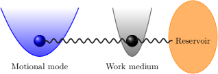
Figure 1: The model. A motional mode is cooled by coupling it to a refrigerator consisting of a driven harmonic oscillator, which acts as a work medium which is externally driven. This oscillator is itself coupled with a bosonic reservoir, which is where all entropy is finally dumped.

From a fundamental perspective, an effort has been made to derive the third law of thermodynamics from first principles. In fact, the impossibility to achieve perfect ground state cooling in finite time (Nernst unattainability principle) has been formally demonstrated However, these proofs, are not of practical significance (as the lower bounds in achievable temperatures are too low indeed) and do not necessarily offer a direct insight on what might be the physical processes imposing the limitations for cooling in actual implementations ticozzi2014 ; wu2013 ; masanes2017 ; wilming2017 .

In this paper we focus on the analysis of the ultimate cooling limit of a class of refrigerators which are externally driven (a situation which is the most important one in practical realizations). We recently presented a detailed analysis of the behavior of a class of quantum refrigerators freitas2017 (linear, externally driven fridges) for which it is possible to identify a very general process as the one responsible for imposing the fundamental limitation for cooling: Such process is nothing but pair creation (a process which is relevant, as discussed below, in other areas of physics and is closely related with the main mechanism behind the so called dynamical Casimir effect, DCE benenti2015 ; freitas2017 ). In fact, our work analyzed a family of linear machines consisting of arbitrary harmonic networks which are parametrically driven while connected with an arbitrary number of bosonic reservoirs, prepared at arbitrary temperatures and characterized by generic spectral densities (see below). The exact solution of this model (obtained without using common approximations such as the weak coupling limit between the system and its environments, the rotating-wave approximation or the Markovian assumption) was used to obtain expressions for the dissipated work and the heat currents flowing from each reservoir into the system. A close examination of this exact solution illuminates the fact that the creation of excitation pairs is dominant at sufficiently low temperatures and is the process enforcing the third law. Interestingly, in our work it was shown that an analysis based on the use of master equations derived in the weak coupling limit would fail to incorporate this fundamental process (because of the fact that the non resonant pair creation processes are not of leading order in the coupling between the system and its environments ). It was also shown that by neglecting this fundamental term, which induces heating of all reservoirs at sufficiently low temperatures, the third law could indeed be violated, as suggested and discussed in Ref. kolavr2012 .

Here, we take advantage of the analysis presented in Ref. freitas2017 and apply it to analyze the limit for cooling a single oscillator (this is possible since, as we mentioned, the results contained in Ref. freitas2017 are valid for environments with arbitrary spectral densities). Analyzing the cooling limit for a single oscillator is relevant in several contexts, such as in the case of cold trapped ions diedrich1989 , trapped atoms hamann1998 , or micromechanical oscillators teufel2011 . The very simple model we will analyze and solve can be naturally viewed as a thermal machine, or a thermal refrigerator (see Fig. 1). The machine is composed of a working medium (a parametrically driven harmonic oscillator) that is in simultaneous contact with two reservoirs. One of these reservoirs has a single harmonic mode that we want to cool. The other reservoir (typically representing the electromagnetic field) is where the energy is dumped. As we will see, the model presented here is an interesting analogy to other more realistic models for laser cooling. Notably, this simple model is sufficient to derive the lowest achievable temperatures in the most relevant physical regimes (and to predict their values in other, still unexplored, regimes). Moreover, it enables a simple interpretation of the heating process limiting laser cooling as the non resonant creation of phonon-photon pairs. The model also enables us to conclude that in any laser cooling process there should be a photon pair production process associated with it, which is closely analogous to the pair production process present in the DCE. In fact, as we show below, our analysis will enable us to estimate the rate of photon pair production that is associated to the typical laser cooling mechanisms with optical frequencies and analyze the possibility of detecting them.

The paper is organized as follows: In Section 2 we present our model to understand laser cooling as a thermodynamical process. We solve the long time dynamics of the model and study its thermodynamical properties. In Section 3 we apply this model to study the cooling of a single motional degree of freedom. We compute the heat currents in this case and find the lowest temperatures that can be achieved. Not only we analyze the two most relevant regimes (Doppler cooling and sideband resolved cooling) but also present possible generalizations where much lower temperatures may be accessible. In Section 4 we analyze the nature of the spectrum of excitations that are created in the photonic reservoir during laser cooling. We show that the photonic spectrum not only consists of two peaks (corresponding to photons emitted during cooling and heating transitions) but also has a broad contribution arising from photon pairs created directly from the driving by a process which is closely connected with the DCE. We finally summarize our results in Section 5.

II A quantum refrigerator as a model for laser cooling

We will present here a simple model that will enable us to study the lowest temperature that can be achieved by laser cooling. In such case, an atom (typically, a two level atom) is illuminated with a laser and three types of degrees of freedom are coupled between each other. The internal (electronic) levels of the atom (a system that we will denote as $\mathcal{S}$ below) couple with the quantized electromagnetic field (whose modes act as an environment which we denote as $\mathcal{E}_{B}$ below). The internal modes also couple with the motional degrees of freedom of the atom, which we consider as an harmonic oscillator and denote as $\mathcal{E}_{A}$ below. The coupling to the laser induces transitions between the atomic levels. Such levels effectively act as a pump (which is driven by the power of the laser) that takes energy out of $\mathcal{E}_{A}$ and dumps it into $\mathcal{E}_{B}$. We will describe a very simple model to study this situation, which has the virtue of being exactly solvable. The main simplification is to replace the internal electronic levels of the atom by a single harmonic mode. Of course, this is a rough approximation which will only be reasonable at sufficiently low temperatures, where only the lowest energy levels of the spectrum of $\mathcal{S}$ will matter. As we will see, the model, whose essential ingredients are shown in Figure 1, is able to accurately predict the correct limiting temperatures obtained for laser cooling in the resolved sideband limit and also in the non-resolved sideband case (and it can also be used to predict new and interesting phenomena).

II.1 The model: Dynamics

Here, we will describe the model and the main properties of its solution. The rigorous derivation of the main equations can be found in Ref. freitas2017 . We consider a parametrically driven oscillator with a Hamiltonian

$$H_{\mathcal{S}}=\frac{p^{2}}{2M}+\frac{1}{2}MV(t)x^{2}.$$ (1)

This system couples with two others, which we arbitrarily treat as ‘reservoirs’ and denote them as $\mathcal{E}_{A}$ and $\mathcal{E}_{B}$. We warn the reader that while in this subsection we will consider the reservoirs to be rather general, in the following section $\mathcal{E}_{A}$ will be assumed to consist of a single oscillator while $\mathcal{E}_{B}$ will consist of an infinite set of bosonic modes (the modes of the electromagnetic field). So, for the moment we consider the reservoirs as consisting of collections of independent oscillators with Hamiltonians

$$H_{\alpha}=\sum_{j}\left(\frac{\pi_{\alpha,j}^{2}}{2m_{j}}+\frac{1}{2}{m_{j}\omega_{\alpha,j}^{2}}q_{\alpha,j}^{2}\right),$$ (2)

where $\alpha=A,B$. The interaction between $\mathcal{S}$ and $\mathcal{E}_{\alpha}$ is considered to be linear in both the coordinates of the system and the environments and is described by the Hamiltonians

$$H_{\mathcal{S},\alpha}=x\>\sum_{k}c_{\alpha,k}\>q_{\alpha,k},$$ (3)

where $c_{\alpha,k}$ are the corresponding coupling constants. Initially, the reservoirs are uncorrelated with $\mathcal{S}$ and are prepared in thermal states at temperatures $T_{\alpha}$.

We assume that the driving is periodic and write

$$V(t)=\sum_{k}V_{k}e^{ik\omega_{d}t}.$$ (4)

We also assume that the coupling with the reservoirs induces a stable stationary regime in the asymptotic limit (the long time limit). In this regime, the state of the system is also periodic and has the same period of the driving, i.e. $T=2\pi/\omega_{d}$).

In what follows, the Green’s function of the system $\mathcal{S}$ will be the essential tool we will use to analyze the asymptotic state (which, being a Gaussian state, is fully characterized by its covariance matrix). The Green function is nothing but the response function of $\mathcal{S}$ defined as the solution of the equation

$$\ddot{G}(t,t^{\prime})+V(t)G(t,t^{\prime})+\int_{0}^{t}d\tau\gamma(t-\tau)\dot{G}(\tau,t)=\delta(t,t^{\prime}),$$ (5)

where the dot denotes a derivative with respect to the first temporal argument and $\gamma(t)$ is the dissipation kernel which incorporates all the effect of the environments on the evolution of the system. This kernel is defined as

$$\gamma(t)=\int_{0}^{\infty}d\omega\frac{I(\omega)}{\omega}\cos(\omega t),$$ (6)

in terms of the so called spectral density of the environment, which is such that $I(\omega)=\sum_{\alpha}I_{\alpha}(\omega)$, with

$$I_{\alpha}(\omega)=\sum_{l}\frac{c_{\alpha,l}^{2}}{Mm_{l}\omega_{l}}.$$ (7)

Below, we will use the Laplace transform of $\gamma(t)$, which we denote as $\hat{\gamma}(s)$) and turns out to be

$$\hat{\gamma}(s)=\int_{0}^{\infty}d\omega\frac{I(\omega)}{\omega}\frac{s}{s^{2}+\omega^{2}}.$$ (8)

As a consequence of the driving, which breaks time homogeneity, the Green function $G(t,t^{\prime})$ does not depend on the time difference $(t-t^{\prime})$ only. In spite of this complication, it is possible to find following relatively simple expression, which is valid in the asymptotic limit freitas2017 :

$$G(t,t^{\prime})=\frac{1}{2\pi}\sum_{k}\int_{-\infty}^{\infty}d\omega A_{k}(\omega)e^{i\omega(t-t^{\prime})}\,e^{ik\omega_{d}t}.$$

As explained in freitas2017 , the derivation of this equation (that we omit here) involves the use of Floquet theory for periodically driven systems. The interpretation of this equation is simple: In the absence of driving, the only surviving term in the Floquet summation is the one with $k=0$. In this case, the Green function depends only on the time difference and $A_{0}(\omega)$ is simply given as $A_{0}(\omega)=g(i\omega)$, where $g(s)$ is the Laplace transform of the undriven damped oscillator, (see below for an explicit formula). When the driving breaks time homogeneity, terms with $k\neq 0$ appear in the Floquet expansion for $G(t,t^{\prime})$ giving rise to a non trivial dependence on the two temporal arguments. The Floquet coefficients $A_{k}(\omega)$ are coupled between each other and satisfy the equations

$$A_{k}(\omega)=\delta_{k,0}\;g\left(i\omega\right)-\sum_{j\neq 0}g\left(i(\omega+k\omega_{d})\right)V_{j}A_{k-j}(\omega).$$ (9)

In all above equations, the Laplace transform of the static Green’s function can be written as

$$g(i\omega)=(-\omega^{2}+V_{R}+i\omega\hat{\gamma}(i\omega))^{-1},$$ (10)

which can also be rewritten as

$$g(i\omega)=(\omega_{0}^{2}-(\omega-i\hat{\gamma}(i\omega)/2)^{2})^{-1}.$$ (11)

Here, $\omega_{0}^{2}=V_{R}-\hat{\gamma}^{2}(i\omega)/4$ and $V_{R}$ is the renormalized frequency of $\mathcal{S}$, which is defined as $V_{R}=V_{0}-\gamma(0)$. The previous definitions clearly imply that both $\omega_{0}$ and $\hat{\gamma}(i\omega)$ do not depend on $\omega$ only when the total spectral density is ohmic, i.e. when $I(\omega)\propto\omega$. In that case, the Green function oscillates with frequency $\omega_{0}$ and decays with a rate $\hat{\gamma}\equiv\gamma$.

II.2 Thermodynamics: Heat currents

To study the exchange of energy between $\mathcal{S}$, $\mathcal{E}_{A}$ and $\mathcal{E}_{B}$ in the stationary regime we first analyze the variation of the expectation value of $H_{\mathcal{S}}$ which satisfies

$$\frac{d\langle H_{\mathcal{S}}\rangle}{dt}=\langle\partial_{t}H_{\mathcal{S}}\rangle-i\sum_{\alpha}\langle[H_{\mathcal{S}},H_{\mathcal{S},\alpha}]\rangle,$$ (12)

(we use $\hbar=1$ here and below). This equation enables us to identify the notions of work and heat which are the two sources for the change in the energy. Thus, the variation of the energy induced by the explicit time dependence of the system’s Hamiltonian is associated with work (more precisely, with power), as

$$\dot{\mathcal{W}}=\langle\partial_{t}H_{\mathcal{S}}/\partial t\rangle.$$ (13)

In turn, the variation of the energy of $\mathcal{S}$ arising from the interaction with each reservoir $\mathcal{E}_{\alpha}$ is associated with the heat flowing into the system per unit time, which we denote as $\dot{\mathcal{Q}}_{\alpha}$ and turns out to be

$$\dot{\mathcal{Q}}_{\alpha}=-i\langle[H_{\mathcal{S}},H_{\mathcal{S},\alpha}]\rangle.$$ (14)

Therefore, the above equation is nothing but the first law of thermodynamics, i.e. $d\langle H_{\mathcal{S}}\rangle/dt=\dot{\mathcal{W}}+\sum_{\alpha}\dot{\mathcal{Q}}_{\alpha}$. In what follows we will study the average values of the work and the heat currents over a driving period (in the limit of long times). These quantities will be respectively defined as $\dot{W}$ and $\dot{Q}_{\alpha}$. In this asymptotic regime, it can be shown that the average heat current $\dot{Q}_{\alpha}$ coincides with the time derivative of the energy of $\mathcal{E}_{\alpha}$ (i.e., $\dot{Q}_{\alpha}=-\dot{\langle H_{\alpha}\rangle}$: the energy lost by $\mathcal{E}_{\alpha}$ is gained by $\mathcal{S}$ over a driving period) freitas2017 . Then, the averaged version of the first law is simply the identity $0=\dot{W}+\sum_{\alpha}\dot{Q}_{\alpha}$.

Using the explicit form of the Hamiltonians, it is relatively simple to express the heat currents in the stationary regime in terms of the Fourier components of the Green function. Again, we do not present the detailed calculation but simply describe the ingredients needed to obtain it (the full derivation can be found in Ref. freitas2017 ). The heat current in the stationary regime can be fully expressed in terms of the covariance matrix of $\mathcal{S}$. Of course, this comes as no surprise since the state of $\mathcal{S}$ is Gaussian in the stationary limit (and therefore it is fully determined by its covariance matrix). The average heat flow has a particularly simple form:

$$\dot{Q}_{\alpha}=\overline{V(t)\sigma_{xp}(t)},$$

where $\sigma_{xp}(t)$ is the position-momentum correlation function of $\mathcal{S}$, defined as $\sigma_{xp}(t)=\langle{\{x(t),p(t)\}\rangle}/2$ (the overbar in the previous equation indicates the average of the product between $V(t)$ and $\sigma_{xp}(t)$ over a period of the oscillation). In the stationary regime, when the memory of the initial state is lost, the correlation function can be fully expressed in terms of the Green function $G(t,t^{\prime})$ as follows:

$$\sigma_{xp}(t)=\frac{1}{2}\int_{0}^{\infty}\int_{0}^{\infty}dt_{1}dt_{2}G(t,t_{1})\nu(t_{1},t_{2})\dot{G}(t,t_{2}),$$

where the noise kernel of the environments is defined as

$$\nu(t)=\int_{0}^{\infty}d\omega\sum_{\alpha}I_{\alpha}(\omega)\coth(\omega/2k_{B}T_{\alpha})\cos(\omega t).$$

Replacing the previous expressions for $G(t,t^{\prime})$, for $V(t)$ and using the set of equations satisfied by the Floquet coefficients $A_{k}(\omega)$ we can derive a particularly simple and physically appealing formula for $Q_{\alpha}$. In fact, in Ref freitas2017 it was shown that the heat current can always be expressed as the sum of three terms

$$\dot{Q}_{\alpha}=\dot{Q}_{\alpha}^{RP}+\dot{Q}_{\alpha}^{RH}+\dot{Q}_{\alpha}^{NRH}.$$

The explicit form of the resonant pumping (RP), the resonant heating (RH) and the non–resonant heating (NRH) contributions to the average heat fluxes will be given below and will enable us to understand the various thermodynamical processes involved. Thus, the first term is:

$$\begin{split}\dot{Q}_{\alpha}^{\text{RP}}&=\sum_{k}\int_{0^{\prime}}^{\infty}d\omega\;\left(\omega\;p^{(k)}_{\beta,\alpha}(\omega)\;N_{\alpha}(\omega)\right.\\ &\left.-(\omega+k\omega_{d})\;p^{(k)}_{\alpha,\beta}(\omega)\;N_{\beta}(\omega)\right)\end{split}$$ (15)

where $N_{\alpha}(\omega)=(e^{\omega/T_{\alpha}}-1)^{-1}$ is the Planck distribution and

$$p_{\alpha,\beta}^{(k)}(\omega)=\frac{\pi}{2}I_{\alpha}(|\omega+k\omega_{d}|)I_{\beta}(\omega)|A_{k}(\omega)|^{2}$$ (16)

is a positive number, proportional to the probability for the system to couple a mode $\omega$ in $\mathcal{E}_{\beta}$ with mode $|\omega+k\omega_{d}|$ in $\mathcal{E}_{\alpha}$. The diagram in Figure 2 describe the processes involved in $\dot{Q}_{\alpha}^{RP}$: excitations are transported between reservoirs after the resonant absorption (or emission) of an energy $k\,\omega_{d}$, a multiple of the quantum of energy of the driving. The origin of the resonant heating $\dot{Q}_{\alpha}^{RH}$ is similar but in this case, as shown in the same Figure, the excitations are transported within the reservoir $\mathcal{E}_{\alpha}$, which always results in heating. The corresponding formula is simply

$$\dot{Q}_{\alpha}^{\text{RH}}=-\sum_{k>0}\int_{0^{\prime}}^{\infty}d\omega\;k\omega_{d}\;p^{(k)}_{\alpha,\alpha}(\omega)\;(N_{\alpha}(\omega)-N_{\alpha}(\omega+k\omega_{d})).$$ (17)

Two points are worth noticing: a) the lower limit of integration in the expression RH current is not $\omega=0$ but $\omega=0^{\prime}=\max\{0,-k\omega_{d}\}$. This is because when $k<0$, the arrival mode exists only if $\omega\geq-k\omega_{d}$. For negative values of the integer $k$, the low frequency part of the spectrum plays no role. As we will see, the low frequency part of the spectrum is crucial in the non resonant processes. b) The negativity of $\dot{\bar{Q}}_{\alpha}^{\text{RH}}$ (which is the reason why this term is always associated with heating) relies on the fact that the Planck distribution decreases with frequency. In fact, population inversion can change the sign of this term.

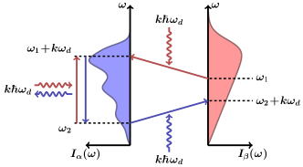
Figure 2: Resonant processes affecting the heat flow in or out of a thermal reservoir are of two types: resonant pumping (RP), associated with $\dot{Q}_{\alpha}^{\text{RP}}$, involves the exchange of energy between different reservoirs, while resonant heating (RH), associated with $\dot{Q}_{\alpha}^{\text{RH}}$, involves the exchange of energy between different modes of the same environment. The total number of excitations in the reservoirs is conserved due to these two mechanisms.

The last term in the heat flow fully contains the contribution of low frequencies. It is the non resonant heating term $\dot{Q}_{\alpha}^{\text{NRH}}$ which reads:

$$\begin{split}&\dot{Q}_{\alpha}^{\text{NRH}}=-\sum_{k>0}\int_{0}^{k\omega_{d}}d\omega\;k\omega_{d}\;p_{\alpha,\alpha}^{(-k)}(\omega)\;\left(N_{\alpha}(\omega)\!+\!\frac{1}{2}\right)-\\ &-\sum_{k>0}\int_{0}^{k\omega_{d}}d\omega\;(k\omega_{d}\!-\!\omega)\;p_{\alpha,\beta}^{(-k)}(\omega)\;\left(N_{\beta}(\omega)\!+\!\frac{1}{2}\right)-\\ &-\sum_{k>0}\int_{0}^{k\omega_{d}}d\omega\;\omega\;p_{\beta,\alpha}^{(-k)}(\omega)\;\left(N_{\alpha}(\omega)\!+\!\frac{1}{2}\right)\end{split}$$ (18)

The non resonant heating does not involve the transport of excitation but the creation of excitation pairs. These processes are depicted in Figure 3. In that Figure we see that these pairs can be created either in different environments or in the same environment giving rise to the three contributions shown in the above formula. The interpretation of the equation is transparent: For each Floquet term (i.e., for each integer $k$), when an excitation with frequency $\omega$ is emitted into one of the reservoirs the second excitation must have a frequency equal to $k\omega_{d}-\omega$. The probability for creating the first excitation has a stimulated contribution (proportional to the mean number of excitations already present in that mode) and also a spontaneous contribution. For each of the possible emission channels, the energy deposited in $\mathcal{E}_{\alpha}$ is either $\omega$, $k\omega_{d}-\omega$ or $k\omega_{d}$. It is worth stressing the fact that Eq. (18) is an exact formula, which is valid both for weak and strong coupling freitas2017 .

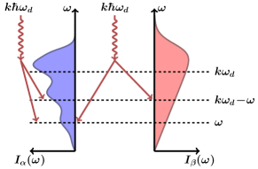
Figure 3: Non Resonant processes affecting the heat flow in and out of each reservoir. They can involve either modes of two different reservoirs or modes of the same reservoir. In all cases, excitations are created in pairs.

II.3 The fundamental limit for cooling

Clearly, $\dot{Q}_{\alpha}^{NRH}\leq 0$ and therefore it corresponds to the heating of all reservoirs. Moreover, when the temperatures of all reservoirs vanish, this is the only term contributing to the heat flow. As a consequence, this term always becomes dominant at sufficiently low temperatures. For this reason, it is responsible for the validity of the third law of thermodynamics. Thus, as discussed in freitas2017 , if the non resonant heating term is not taken into account (which is clearly erroneous at low temperatures) the third law could indeed be violated, as suggested recentlykolavr2012 .

Identifying the process of pair creation as the one imposing the fundamental limit for cooling may sound a bit exotic. As far as we know, this process is never mentioned in the most relevant texts on laser cooling cirac1992 ; eschner2003 as the one to blame for the fact that such type of cooling process cannot reach zero temperature. On the other hand, pair production through parametric driving is a well known phenomenon that has been identified as relevant in many other contexts which seem to be unrelated to the one we are analyzing. For example, the spacetime dynamics induces cosmological pair creation birrell1984 , which play an important role in the history of our Universe. In fact, pair creation due to parametric driving is particularly relevant during the relating stage of inflationary models of the early Universe mazzitelli1989 ). Also, the motion of the mirrors that form a cavity excites the vacuum and induces the creation of pairs of photons inside the cavity. This process, that is known as the dynamical Casimir effect (DCE) dodonov2010 ; birrell1980 ; birrell1984 was recently studied both with theoretical and experimental methods dodonov2010 ; wilson2011 ; lahteenmaki2013 . The analogy between our analysis and the typical setup used to analyze the DCE is clear: In fact, when there is a single reservoir, our equation (18) is identical to the one describing the power spectrum of created pairs in the DCE. We can interpret this as a consequence of the fact that, in our case, the driving of $\mathcal{S}$ effectively act as some sort of moving boundary conditions for the environmental modes and, in this way, it induces pair creation. This is a rich analogy and we will exploit it below, where we will show that pair creation is the natural process to be blamed for imposing the lowest achievable temperature in the cooling of a single motional mode as it is typically done in laser cooling.

III Cooling a single motional mode

The previous expressions are valid for arbitrary spectral densities. We will apply them here to analyze the limits for cooling of a single motional mode, whose frequency we denote as $\omega_{m}$. For this, we consider the spectral density of $\mathcal{E}_{A}$ to be such that $I_{A}(\omega)=\tilde{I}_{A}\,\delta(\omega-\omega_{m})$, where $\tilde{I}_{A}$ is a constant. In this case, the relevant processes for cooling and heating of $\mathcal{E}_{A}$ are displayed in Figure 4 (where a spectral density peaked about $\omega_{m}$ was used for illustrative purposes). Clearly, the RH process is absent since $\mathcal{E}_{A}$ consists only of a single mode. The lowest achievable temperature can be estimated by analyzing the condition under which the heating and cooling terms balance each other. Using the above equations it is simple to compute this ratio as

$$\left|\frac{\dot{Q}^{\text{RP}}_{A}}{\dot{Q}_{A}^{NRH}}\right|=\frac{\bar{n}}{1+\bar{n}}\frac{\sum_{k>0}I_{\beta}(k\omega_{d}+\omega_{m})|A_{k}(\omega_{m})|^{2}}{\sum_{k>0}I_{\beta}(k\omega_{d}-\omega_{m})|A_{-k}(\omega_{m})|^{2}},$$ (19)

where $\bar{n}=N_{A}(\omega_{m})$ is the average number of excitations in the motional mode (the one that is being cooled). In order to simplify our analysis, we neglected the heating term appearing in the resonant pumping current $\dot{Q}^{RP}$. By doing this, we study the most favorable condition for cooling, assuming that the pumping of excitations from $\mathcal{E}_{B}$ into $\mathcal{E}_{A}$ is negligible. This is equivalent to assuming that the temperature of $\mathcal{E}_{B}$ is $T_{B}\simeq 0$. Although this is a reasonable approximation in many cases (such as the cooling of a single trapped ion) we should have in mind that by doing this, the limiting temperature we will obtain should be actually viewed as a lower bound to the actual one. Thus, the condition defining the lowest bound is that the ratio between the RP and NRH currents is of order unity. Using the previous expressions, it is simple to show that this implies that

$$\frac{1}{\bar{n}}=\frac{\sum_{k>0}I_{B}(k\omega_{d}+\omega_{m})|A_{k}(\omega_{m})|^{2}}{\sum_{k>0}I_{B}(k\omega_{d}-\omega_{m})|A_{-k}(\omega_{m})|^{2}}-1.$$ (20)

To pursue our analysis, we need an expression for the Floquet coefficients $A_{k}(\omega)$. This can be obtained under some simplifying assumptions. In fact, if the driving is harmonic (i.e. if $V(t)=V_{0}+V(e^{i\omega_{d}t}+e^{-i\omega_{d}t})$) and that its amplitude is small (i.e. if $V\ll V_{0}$), we can use perturbation theory to compute the Floquet coefficients to leading order in $V$. In fact, by doing this we find that the only non vanishing terms are the ones corresponding to $k=\pm 1$ which read

$$A_{\pm 1}(\omega_{m})\approx-g(i(\omega_{m}\pm\omega_{d}))V\,g(i\omega_{m}).$$ (21)

Using this, we find that

$$\frac{1}{\bar{n}}=\frac{I_{B}(\omega_{d}+\omega_{m})|g(i(\omega_{d}+\omega_{m}))|^{2}}{I_{B}(\omega_{d}-\omega_{m})|g(i(\omega_{d}-\omega_{m}))|^{2}}-1$$ (22)

The final step of our derivation requires the use of an expression for $g(s)$ (the propagator of the undriven oscillator). For this we use a semi phenomenological approach by simply assuming that, in the absence of driving, the coupling with the reservoirs induces an exponential decay of the oscillations of $\mathcal{S}$. In this case, we can simply write $g(i\omega)=1/((\omega-i\gamma/2)^{2}-\omega_{0}^{2})$, where $\gamma$ is the decay rate and $\omega_{0}$ is the renormalized frequency of $\mathcal{S}$. As mentioned above, this same expression is obtained if we assume that $\mathcal{S}$ behaves as if it were coupled with a single ohmic environment (this is indeed a reasonable assumption in many cases but it certainly requires that the back action of $\mathcal{E}_{A}$ on $\mathcal{S}_{S}$ is negligible in the long time limit). Then, we can simply write that

$$|g(i\omega)|^{2}=\frac{1}{(\omega^{2}-\omega_{0}^{2}+\gamma^{2})^{2}+4\gamma^{2}\omega_{0}^{2}}.$$ (23)

Using this, we find the following expression for the lowest achievable number of excitations in $\mathcal{E}_{A}$:

$$\frac{1}{\bar{n}}=\frac{I_{B}(\omega_{d}+\omega_{m})}{I_{B}(\omega_{d}-\omega_{m})}\frac{((\omega_{d}-\omega_{m})^{2}-\omega_{0}^{2}+\gamma^{2})^{2}+4\omega_{0}^{2}\gamma^{2}}{((\omega_{d}+\omega_{m})^{2}-\omega_{0}^{2}+\gamma^{2})^{2}+4\omega_{0}^{2}\gamma^{2}}-1.$$ (24)

This relatively simple formula, is an important result of our paper. It show that the asymptotic value of $\bar{n}$ depends on four parameters: $\omega_{0}$, $\omega_{m}$, $\gamma$ and $\omega_{d}$. The first three of them characterize the system while $\omega_{d}$ can be adjusted to minimize $\bar{n}$. As shown below, the optimal driving frequency depends on the other parameters in an interesting manner. In particular, we will study two physically important regimes where the decay rate satisfies either that $\gamma\ll\omega_{m}$ (the limit of resolved sidebands) or $\gamma\gg\omega_{m}$ (the limit of non resolved sidebands). In both cases we will show that our expression for the limiting temperature coincides with the one obtained when studying the limit for laser cooling.

III.1 The limit of sideband resolved laser cooling

Let us analyze the conditions under which it is possible to achieve ultra low temperatures, i.e. temperatures such that $\bar{n}\ll 1$. In that case, it is simple to show that the optimal driving frequency is the one for which the denominator appearing in the expression for $1/\bar{n}$ is minimal. Thus, assuming that the ratio $I_{B}(\omega_{d}-\omega_{m})/I_{B}(\omega_{d}+\omega_{m})$ is a slowly varying function of $\omega_{d}$ (which is certainly the case when $\omega_{d}\gg\omega_{m}$ such as in the case of a trapped ion), the optimal driving frequency is such that $\omega_{d}=\sqrt{\omega_{0}^{2}-\gamma^{2}}-\omega_{m}$. In this case, the lowest achievable temperature is such that

$$\begin{split}\bar{n}&=\frac{\gamma^{2}\omega_{0}^{2}}{4\omega_{m}^{2}\omega_{d}^{2}+\omega_{0}^{2}\gamma^{2}}\frac{I_{\beta}(\omega_{d}-\omega_{m})}{I_{\beta}(\omega_{d}+\omega_{m})}\\ &\approx\frac{\gamma^{2}}{4\omega_{m}^{2}}\frac{\omega_{0}^{2}}{(\omega_{0}-\omega_{m})^{2}}\frac{I_{B}(\omega_{0}-2\omega_{m})}{I_{B}(\omega_{0})},\end{split}$$ (25)

where the approximation $\gamma\ll\omega_{0}$ was used to obtain the last expression. In this case $\omega_{d}\approx\omega_{0}-\omega_{m}$, which implies that the optimal situation is achieved when the driving is resonant with the red detuned lateral sideband of the carrier frequency $\omega_{0}$. Clearly, the condition $\bar{n}\ll 1$ can only be satisfied if $\gamma\ll\omega_{m}$, which is nothing but the condition for resolved sidebands. Notably, the above expression for $\bar{n}$ coincides with previously known formulae for the lowest achievable temperature in sideband resolved laser cooling, which were obtained by completely different methods. In fact, in that case a further simplification is possible as laser cooling is typically done in the optical regime for $\omega_{0}$ and $\omega_{d}$ (which are therefore much larger than $\omega_{m}$, which is typically in the r.f. domain). Then, the ratio $I_{B}(\omega_{d}-\omega_{m})/I_{B}(\omega_{d}+\omega_{m})$ is of order unity and, therefore, we have that the lowest temperature is such that $\bar{n}=\gamma^{2}/4\omega_{m}^{2}$. Our formula is clearly more general and can be applied in other cases, as discussed below.

III.2 The limit of Doppler cooling

Let us now study a different regime, where the cooling does not achieve ultra low temperatures (i.e., the condition $\bar{n}\ll 1$ is not satisfied). If we neglect the contribution arising from the spectral densities (which, as above, is a reasonable approximation whenever $\omega_{0}\gg\omega_{m}$, like in the optical regime) the asymptotic value of the occupation number is

$$\bar{n}=\frac{\left((\omega_{d}+\omega_{m}-\omega_{0})^{2}+\gamma^{2}\right)\left((\omega_{d}+\omega_{m}+\omega_{0})^{2}+\gamma^{2}\right)}{8\omega_{d}\omega_{m}\left(\omega_{0}^{2}-\omega_{m}^{2}-\gamma^{2}-\omega_{d}^{2}\right)}$$

Cooling is possible only if the condition $\omega_{0}^{2}>\omega_{m}^{2}+\gamma^{2}+\omega_{d}^{2}$ is satisfied (notice that this implies that $\omega_{0}$ must be larger than $\omega_{d}$, $\omega_{m}$ and $\gamma$). The above expression (which is valid whenever the spectral density varies slowly with $\omega_{m}$) can be used to study the case where $\gamma\gg\omega_{m}$, which physically very important. In fact, this regime corresponds to the Doppler cooling limit, where the sidebands are not resolved. In this case, the optimal driving frequency can be shown to be $\omega_{d}=\omega_{0}-\gamma$ and the limiting temperature turns out to be

$$\bar{n}=\frac{\gamma}{2\omega_{m}}$$

In this case, the cooling condition is satisfied whenever $2\gamma\omega_{d}\geq\omega_{m}^{2}$ (analogously, in the sideband resolved case the cooling condition requires that $2\omega_{m}\omega_{d}\geq\gamma^{2}$, which is naturally satisfied). Thus, by applying a single formula in two different situations we obtained the limiting temperatures in the most relevant regimes for laser cooling. This seems to indicate that the mechanism that is responsible for stopping laser cooling is pair creation. Let us analyze this in some detail.

III.3 The role of pair creation in laser cooling

According to our analysis, the origin of the lowest achievable temperature in the class of refrigerators we analyzed is imposed by pair creation from the driving. This is certainly not the typical explanation for the reason why laser cooling stops. However, we will see now that pair creation has a natural role in laser cooling. Thus, we will see that pair creation is certainly not an exotic but an essential process in this case. The relevant processes that play a role in the resonant pumping and non resonant heating currents are shown in Fig. 4 (for $\omega_{d}>\omega_{m}$).

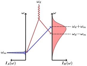
Figure 4: Relevant processes contributing to the heat current of reservoir $\mathcal{E}_{A}$ when $\omega_{d}>\omega_{m}$ and $T_{B}\simeq 0$.

Thus, the resonant pumping of energy out of $\mathcal{E}_{A}$ (blue arrow in Figure 4) corresponds to a removal of a motional excitation (a phonon) and its transfer to the photonic environment. A phonon with frequency $\omega_{m}$ disappears in $\mathcal{E}_{A}$ and a photon with frequency $\omega_{0}$ appears in $\mathcal{E}_{B}$. This is possible by absorbing energy $\omega_{d}=\omega_{0}-\omega_{m}$ from the driving. This process is usually visualized in a different way in the standard literature of laser cooling eschner2003 , as shown in Fig. 5.

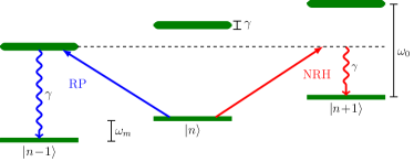
Figure 5: Usual depiction of the staircase of energy levels and the transitions between them involved in Doppler and sideband laser cooling (actually, there are other non resonant processes in play, see eschner2003 )

This Figure shows the energy levels of the combined system formed by $\mathcal{E}_{A}$ and $\mathcal{S}$. In our case, both systems are oscillators and each one of them has an infinite number of energy levels. However, we only pay attention to the lowest levels of $\mathcal{S}$. Thus, the resonant pumping process (RP) takes the system from the lowest energy level of $\mathcal{S}$ with $n$ phonons into the excited level of $\mathcal{S}$ with $(n-1)$ phonons. Then, as $\mathcal{S}$ is coupled to the environment $\mathcal{E}_{B}$, it decays from the excited $|e\rangle$ to the ground ($|g\rangle$) state by emitting an excitation (a photon) in $\mathcal{E}_{B}$, whose frequency is $\omega_{0}$. This is the key process responsible for sideband resolved laser cooling. The system is cooled because resonant pumping forces the combined $\mathcal{E}_{A}-\mathcal{S}$ system to move down in the staircase of energy levels.

However, if resonant pumping were the only relevant process, the above argument would induce us to conclude that laser cooling could achieve zero temperature: by going down the staircase of energy levels, $\mathcal{S}$ would end up in its ground state and the motional mode would end up with $n=0$ phonons. The reason why this does not happen is the existence of non resonant heating. This process is described as NRH in Fig. 5. It corresponds to the creation of a pair of excitations consisting of a phonon and a photon. The phonon, has frequency $\omega_{m}$ while the photon should have frequency $\omega_{d}-\omega_{m}$. We may choose to describe this pair creation process as a sequence of heating transitions that moves the combined $\mathcal{S}$–$\mathcal{E}_{A}$ system up along the staircase of energy levels. This can be done as follows: Suppose that we start from $n$ phonons in the motional state and $\mathcal{S}$ in the ground state $|g\rangle$. Then, $\mathcal{S}$ can absorb energy $\omega_{d}$ from the driving and jump into a virtual state from which it can decay back into $|g\rangle$ but with a motional state with $n+1$ phonons. This heating transition has the net effect of creating a phonon and emitting a photon. As we wrote before, and we stress again, laser cooling stops (in this sideband resolved limit) when the resonant cooling transitions are compensated by non resonant heating transitions where energy is absorbed from the driving and is split between two excitations: one in the motional mode (a phonon) and one in the environmental mode (a photon). As a consequence of the non resonant transitions, the motion heats up. The limiting temperature is achieved when the resonant (RP) and non resonant (NRH) processes balance each other.

Of course, the way in which we are describing the processes involved in laser cooling (both the cooling and the heating transitions) is not the standard one but provides a new perspective and some new predictions, which we will discuss below.

III.4 Ultra low temperatures for structured reservoirs

A first generalization of the standard results for the limiting temperatures achieved in laser cooling arises if we can manipulate the environmental spectral density. In that case, new results emerge, which we analyze now. In fact, the properties of spectral density of the reservoir may be very relevant in establishing the lowest achievable temperature in some cases. Thus, this is because of the presence of the ratio $I_{B}(\omega_{d}-\omega_{m})/I_{B}(\omega_{d}+\omega_{m})$ in Eq. (24). As we will see, this ratio may play an interesting role in certain cases. If the spectral density is a monotonic function of the frequency (at least in a relevant band around $\omega_{d}$), the ratio is always smaller than unity. As we mentioned above, when $\omega_{m}$ is much smaller than $\omega_{d}$, the ratio is close to unity and can be neglected. However, when $\omega_{m}$ is of the same order of magnitude than $\omega_{0}$, the ratio may be very small and substantially modify the minimal occupation number that the cooling mechanism can achieve.

Let us analyze this now. We take $\omega_{0}$ and $\omega_{m}$ to be similar. As before, we assume we are in an underdamped regime where $\omega_{0}\gg\gamma$. Therefore, we also have $\omega_{m}\gg\gamma$ and the resolved sideband condition is satisfied. Thus, the optimal driving frequency is $\omega_{d}=\omega_{0}-\omega_{m}$ and the minimum occupation number is given above by Eq. (24). If the spectral density is such that $I_{B}(\omega)\propto\omega^{\kappa}$, then Eq. (24) becomes:

$$\bar{n}_{\text{min}}=\frac{1}{4}\left(\frac{\Gamma}{\omega_{m}}\right)^{2}\frac{(1-2\omega_{m}/\omega_{0})^{\kappa}}{(1-\omega_{m}/\omega_{0})^{2}}.$$ (26)

For $\kappa\geq 1$ (Ohmic and super-Ohmic spectral densities), the factor $f=(1-2\omega_{m}/\omega_{0})^{\kappa}/(1-\omega_{m}/\omega_{0})^{2}$ is always less than unity. As a consequence, the minimum achievable temperature is lower than the one given by the standard formula for sideband cooling. Instead, for sub-Ohmic spectral densities, the condition $f<1$ is satisfied only when $\omega_{m}/\omega_{0}$ is larger than a critical value. For example, if $\kappa=1/2$, we have $0<f<1$ only if $0.457<\omega_{m}/\omega_{0}<0.5$. In turn, for highly sub-Ohmic environments with $\kappa\ll 1$, the condition $f<1$ is satisfied only in a very narrow band (defined as $1/2(1-1/2^{2/\kappa})<\omega_{m}/\omega_{0}<1/2$.

If the environmental spectral density is such that $I(\omega=0)=0$, then the lowest value of $\bar{n}$ obtained from Eq. 24 tends to zero when $\omega_{m}\to\omega_{0}/2$. In fact, in this case the pair creation mechanism described above is suppressed (because the excitation would have to be created at very low frequencies, where the environment has no available modes). This result may lead us to the erroneous conclusion than zero temperature could be achieved. Indeed, this is not the case because when $\omega_{d}=\omega_{m}$, the non resonant heating current is dominated by the next to leading order term in the Floquet index (i.e., $k=\pm 2$). Thus, in this case the pairs of excitations are created by absorbing energy $2\omega_{d}$ from the driving. In fact, this energy is enough to create an excitation in the motion and another excitation in the environment at frequency $\omega_{m}$. Of course, this process is of higher order in the driving amplitude $V$. In this case, going back to Eq. 20 we can estimate the correct limiting temperature. Thus, using the fact that, when $\omega_{d}=\omega_{m}$ we have $A_{-2}(\omega_{m})=g(-i\omega_{m})VA_{-1}(\omega_{m})$ we obtain

$$\bar{n}|_{\omega_{0}=2\omega_{m}}\approx\frac{\gamma^{2}}{\omega_{m}^{2}}\frac{I_{B}(\omega_{m})}{I_{B}(2\omega_{m})}\frac{64V^{2}}{9\omega_{m}^{4}}.$$ (27)

Therefore, Eq. (24) is valid only if $\omega_{m}$ is not too close to $\omega_{0}/2$. Otherwise, higher order processes must be taken into account.

These considerations are not relevant for the majority of sideband cooling implementations, where the motional frequency $\omega_{m}$ is several orders of magnitude lower than the central system frequency $\omega_{0}$leibfried2001 ; vuletic1998 ; teufel2011 . However, they might be of interest for systems of superconducting qubits coupled with radio frequency cavities. In that case, one could use the qubit to pump energy away from one cavity dumping it in a second one. In this type of systems the frequencies of these two objects can be selected by design, and they can be of the same order (in fact, in this type of system, the DCE was already observedwilson2011 ; lahteenmaki2013 ).

IV Power spectrum of the emitted radiation:

As was explained in the previous sections, in the usual presentation of laser cooling the heating mechanisms preventing the perfect preparation of the motional ground state are understood as inelastic scattering events involving transitions to virtual electronic levels followed by spontaneous emissionseschner2003 . When one of these processes takes place, the overall effect is the creation of a motional excitation and the emission of a photon with the frequency reduced by $\omega_{m}$ with respect to the incident radiation.

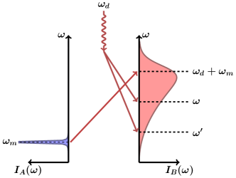
Figure 6: Relevant processes contributing to the heat current of reservoir $\mathcal{E}_{B}$ when $\omega_{d}>\omega_{m}$ and $T_{B}\simeq 0$. Pairs of photons are created at frequencies $\omega$ and $\omega^{\prime}$ such that $\omega+\omega^{\prime}=\omega_{d}$.

From our point of view, this process can also be understood as a particular case of the pairs creation mechanism, analogous to the one present in the DCE. Thus, the motional excitation and the emitted photon, whose frequency is $\omega_{d}-\omega_{m}$ are analogous to a dynamical Casimir pair. However, there is another aspect of the cooling process in which the pair creation process plays a role. This can be seen by analyzing the heat current entering the reservoir $\mathcal{E}_{B}$, which represent the electromagnetic field. In fact, during the cooling process there will be three types of photons which will be emitted in $\mathcal{E}_{B}$. Firstly, we will find photons with the carrier frequency $\omega_{0}$ which are produced during the resonant cooling transitions (where a phonon is transformed into a photon by absorbing energy from the driving). Secondly, we will find the photons emitted during the heating transitions which, as described above, have frequency $\omega_{0}-2\omega_{m}$. These two processes were described above and are associated with the diagrams presented in Figure 4 and 5. But there will be a third class of photons which are emitted in pairs directly from the driving.

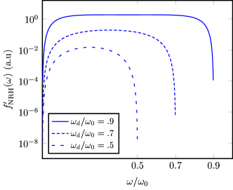
Figure 7: Power spectrum for the creation of photon pairs directly into the electromagnetic field (for $I_{B}(\omega)\propto\omega^{3}$).

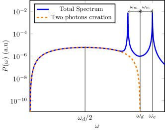
Figure 8: Full power spectrum for the heat current entering the electromagnetic field (for $I_{B}(\omega)\propto\omega^{3}$).

All the above mentioned contributions to the electromagnetic radiation during the cooling process can be analyzed from our previous formulae. In fact, the power spectrum of the energy dumped into the EM field can be read from the integrand of Eqs. (15), (17) and (18). They precisely contain the three contributions we mentioned above. The first one comes from the resonant pumping (RP) of energy from reservoir $\mathcal{E}_{A}$ to $\mathcal{E}_{B}$, which creates photons at frequency $\omega_{d}+\omega_{m}$. Thus, if $f_{\text{RP}}(\omega)$ is the number of photons per unit of time created at frequency $\omega$ by this process, we have, for $\omega>\omega_{d}$:

$$f_{\text{RP}}(\omega)=\frac{\pi}{2}I_{B}(\omega)I_{A}(\omega-\omega_{d})|A_{1}(\omega-\omega_{d})|^{2}N_{A}(\omega-\omega_{d})$$ (28)

In the same way, the number of photons per unit of time created at frequency $\omega$ by the pair creation of Figure 4 is:

$$f_{\text{NRH}}(\omega)=\frac{\pi}{2}I_{B}(\omega)I_{A}(\omega_{d}-\omega)|A_{-1}(\omega)|^{2}\left[N_{A}(\omega_{m})+1\right],$$ (29)

for $\omega<\omega_{d}$. Finally, for the pair creation of Figure 6 we have a number of photons per unit time given by:

$$f^{\prime}_{\text{NRH}}(\omega)=\frac{\pi}{4}I_{B}(\omega)I_{B}(\omega_{d}-\omega)|A_{-1}(\omega)|^{2}$$ (30)

This last contribution, in contrast with the other two, is not spectrally narrow but very broad. The power spectrum associated with the photon pairs is plotted in Figure 7, where we can see that these photons are symmetrically distributed around $\omega_{d}/2$. The total power spectrum if plotted in Figure 8 for the parameters $\omega_{m}/\omega_{0}=.1$, $\gamma/\omega_{0}=10^{-2}$, and $\omega_{d}=\omega_{0}-\omega_{m}$ (since this is optimal for $\gamma/\omega_{m}\ll 1$). Also, for this plot, the Dirac delta in $I_{A}(\omega)$ was replaced by a Lorentzian function $(\Gamma_{m}/(2\pi))/((\omega-\omega_{0})^{2}+(\Gamma_{m}/2)^{2})$ with a width which was chosen as $\Gamma_{m}=10^{-2}\omega_{m}$. When the motional mode reaches its minimal temperature, the two main spectral peaks located at frequencies $\omega_{d}\pm\omega_{m}$ have the same height (since the number of photons emitted during cooling transitions should be the same as the number of photons emitted during heating transitions). We stress that our derivation only rigorously applies to a system made out of harmonic modes so the relation between our results and those obtained for the actual model for laser cooling could be questionable.

However, we can try to estimate the ratio $R$ between the total number of Casimir photons and the number of photons associated with the main peaks when the parameters are of the same order of magnitude than the ones typically involved in the Doppler cooling of a trapped ion. For this, we consider the spectral density of $\mathcal{E}_{B}$ to be such that $I_{B}(\omega)=\tilde{I}_{B}(\omega/\omega_{0})^{3}$ (as it is the case for the electromagnetic modes in open space). As it is the case in the Doppler cooling limit, we also consider that $\omega_{0}\gg\gamma\gg\omega_{m}$. Thus, we obtain:

$$R=\frac{\int f^{\prime}_{\text{NRH}}(\omega)d\omega}{\int f_{\text{NRH}}(\omega)d\omega}\simeq\frac{1}{4}\frac{\omega_{m}}{\omega_{0}}\frac{\tilde{I}_{B}}{\tilde{I}_{A}}\gamma.$$ (31)

To pursue, we need to find an expression for the ratio between the constants appearing in the spectral densities of $\mathcal{E}_{A}$ and $\mathcal{E}_{B}$ (i.e. an expression for $\tilde{I}_{B}/\tilde{I}_{A}$). This can be done by choosing the parameters of our model in such a way that they mimic the ones corresponding to the Hamiltonian of a single trapped ion. Then, it is simple to see that we should choose $\tilde{I}_{A}\propto\eta^{2}\Omega^{2}$ and $\tilde{I}_{B}\propto\gamma$, where $\Omega$ is the Rabi frequency (which is proportional to square root of the laser power) and $\eta$ is the Lamb-Dicke parameter (the ratio between the spread of the ground state wave function and the laser wavelength). Then, we find that

$$\frac{\tilde{I}_{B}}{\tilde{I}_{A}}=\frac{\gamma}{\Omega^{2}\eta^{2}},$$

For the typical cooling process of Calcium ions, the experimental parameters are roos1999 : $\omega_{m}=2\pi\times 5\text{Mhz}$, $\omega_{0}=2\pi\times 755\text{Thz}$ (corresponding to the $397\text{nm}$ $S_{1/2}\to P_{1/2}$ transition of a calcium ion), $\gamma=2\pi\times 20\text{Mhz}$, $\Omega=2\pi\times 1\text{Mhz}$ and $\eta=0.078$. Using these values we obtain that $R\simeq 10^{-4}$. Also, under these conditions approximately $3\times 10^{3}$ photons per second are emitted in the cooling and heating transitions (which, in this case, do not form two peaks in the emission spectrum but lie inside a single line whose width is proportional to $\gamma$). Therefore, the number of created pairs is exceedingly low: less than 1 pair of photons per second are produced (in all directions), which makes their observation impossible in practice (for a single trapped ion). However, to find out if the photon pairs created during the cooling of a trapped ion can be observed, it is necessary to perform a careful analysis of a realistic model (which is out of the scope of this paper).

V Conclusions

We have analyzed the solution of a simple mechanical model which, when studied in the quantum (low temperature) regime, can be use to understand and illustrate the most important aspects of the process of laser cooling. Analyzing in detail the thermodynamical properties of linear thermal refrigerators (parametrically driven) we estimated the lowest achievable temperatures (and the optimal driving frequency) for the most relevant limiting cases: the resolved sideband regime and the Doppler (non resolved sideband) limit. The estimated temperatures coincide with the usual expressions available in the laser cooling literature eschner2003 : $\bar{n}=(\gamma/\omega_{m})^{2}$ when $\gamma\ll\omega_{m}$ and $\bar{n}=\gamma/\omega_{m}$ when $\gamma\gg\omega_{m}$. The virtue of our analysis in our opinion, is that it enables us to understand the process that fixes the lowest achievable temperature in a simple thermodynamical way: there is a fundamental heating process which dominates any driven refrigerator at sufficiently low temperatures and consists of non resonant creation of excitations in the low frequency part of the environmental spectrum (frequencies lower than the driving frequency). Creation of phonon-photon pairs unavoidably heat the motional degree of freedom which is being cooled. It has a counterpart in the photon-photon pairs which are dumped in the electromagnetic environment in a way which is entirely analogous to the dynamical Casimir effect. As we showed, the usual limiting temperatures for laser cooling are obtained provided we focus in the optical regime (where both the driving frequency and the carrier $\omega_{0}$ are much larger than the motional frequency which is being cooled). In a different regime, our analysis enables to predict other limits, where the lowest temperature is modified by the spectral properties of the environment where the entropy is dumped.

We acknowledge support of ANPCyT, CONICET and UBACyT (Argentina).

References

- [1] Jürgen Eschner, Giovanna Morigi, Ferdinand Schmidt-Kaler, and Rainer Blatt. Laser cooling of trapped ions. JOSA B, 20(5):1003–1015, 2003.
- [2] Aaron D O’Connell, Max Hofheinz, Markus Ansmann, Radoslaw C Bialczak, Mike Lenander, Erik Lucero, Matthew Neeley, Daniel Sank, H Wang, M Weides, et al. Quantum ground state and single-phonon control of a mechanical resonator. Nature, 464(7289):697–703, 2010.
- [3] JD Teufel, T Donner, Dale Li, JW Harlow, MS Allman, K Cicak, AJ Sirois, JD Whittaker, KW Lehnert, and RW Simmonds. Sideband cooling of micromechanical motion to the quantum ground state. Nature, 475(7356):359–364, 2011.
- [4] Vladan Vuletić, Cheng Chin, Andrew J Kerman, and Steven Chu. Degenerate raman sideband cooling of trapped cesium atoms at very high atomic densities. Physical Review Letters, 81(26):5768, 1998.
- [5] Armen E Allahverdyan, Karen V Hovhannisyan, Dominik Janzing, and Guenter Mahler. Thermodynamic limits of dynamic cooling. Physical Review E, 84(4):041109, 2011.
- [6] Amikam Levy, Robert Alicki, and Ronnie Kosloff. Quantum refrigerators and the third law of thermodynamics. Physical Review E, 85(6):061126, 2012.
- [7] Lian-Ao Wu, Dvira Segal, and Paul Brumer. No-go theorem for ground state cooling given initial system-thermal bath factorization. Scientific reports, 3, 2013.
- [8] Francesco Ticozzi and Lorenza Viola. Quantum resources for purification and cooling: fundamental limits and opportunities. Scientific reports, 4, 2014.
- [9] Lluís Masanes and Jonathan Oppenheim. A general derivation and quantification of the third law of thermodynamics. Nature Communications, 8, 2017.
- [10] Henrik Wilming and Rodrigo Gallego. The third law as a single inequality. arXiv preprint arXiv:1701.07478, 2017.
- [11] Nahuel Freitas and Juan Pablo Paz. Fundamental limits for cooling of linear quantum refrigerators. Phys. Rev. E, 95(1):012146, 2017.
- [12] Giuliano Benenti and Giuliano Strini. Dynamical casimir effect and minimal temperature in quantum thermodynamics. Physical Review A, 91(2):020502, 2015.
- [13] Michal Kolář, David Gelbwaser-Klimovsky, Robert Alicki, and Gershon Kurizki. Quantum bath refrigeration towards absolute zero: Challenging the unattainability principle. Physical review letters, 109(9):090601, 2012.
- [14] F Diedrich, JC Bergquist, Wayne M Itano, and DJ Wineland. Laser cooling to the zero-point energy of motion. Physical Review Letters, 62(4):403, 1989.
- [15] SE Hamann, DL Haycock, G Klose, PH Pax, IH Deutsch, and Poul S Jessen. Resolved-sideband raman cooling to the ground state of an optical lattice. Physical Review Letters, 80(19):4149, 1998.
- [16] J Ignacio Cirac, R Blatt, Peter Zoller, and WD Phillips. Laser cooling of trapped ions in a standing wave. Physical Review A, 46(5):2668, 1992.
- [17] Nicholas David Birrell and Paul Charles William Davies. Quantum fields in curved space. Number 7. Cambridge university press, 1984.
- [18] FD Mazzitelli, JP Paz, and C El Hasi. Reheating of the universe and evolution of the inflaton. Physical Review D, 40(4):955, 1989.
- [19] VV Dodonov. Current status of the dynamical casimir effect. Physica Scripta, 82(3):038105, 2010.
- [20] ND Birrell and PCW Davies. Conformal-symmetry breaking and cosmological particle creation in 4 theory. Physical Review D, 22(2):322, 1980.
- [21] CM Wilson, Göran Johansson, Arsalan Pourkabirian, Michael Simoen, JR Johansson, Tim Duty, F Nori, and Per Delsing. Observation of the dynamical casimir effect in a superconducting circuit. Nature, 479(7373):376–379, 2011.
- [22] Pasi Lähteenmäki, GS Paraoanu, Juha Hassel, and Pertti J Hakonen. Dynamical casimir effect in a josephson metamaterial. Proceedings of the National Academy of Sciences, 110(11):4234–4238, 2013.
- [23] D Leibfried, C Roos, P Barton, H Rohde, S Gulde, AB Mundt, G Reymond, M Lederbauer, F Schmidt-Kaler, J Eschner, et al. Experiments towards quantum information with trapped calcium ions. In AIP Conference Proceedings, volume 551, pages 130–142. AIP, 2001.
- [24] Ch Roos, Th Zeiger, H Rohde, HC Nägerl, J Eschner, D Leibfried, F Schmidt-Kaler, and R Blatt. Quantum state engineering on an optical transition and decoherence in a paul trap. Physical Review Letters, 83(23):4713, 1999.