Recent advances on the global regularity
for irrotational water waves

Abstract.

We review recent progress on the long-time regularity of solutions of the Cauchy problem for the water waves equations, in two and three dimensions.

We begin by introducing the free boundary Euler equations and discussing the local existence of solutions using the paradifferential approach, as in [7, 1, 2]. We then describe in a unified framework, using the Eulerian formulation, global existence results for three dimensional and two dimensional gravity waves, see [70, 146, 145, 87, 5, 6, 79, 80, 136], and our joint result with Deng and Pausader [60] on global regularity for the 3D gravity-capillary model.

We conclude this review with a short discussion about the formation of singularities, and give a few additional references to other interesting topics in the theory.

Contents

1. 1 Introduction
2. 2 Local well-posedness
3. 3 Global regularity and asymptotic behavior
4. 4 Formation of singularities and other topics

1. Introduction

The study of the motion of water waves, such as those on the surface of the ocean, is a classical question, and one of the main problems in fluid dynamics. The origins of water waves theory can be traced back at least to the work of Laplace and Lagrange, Cauchy [28] and Poisson, and then Russel, Green and Airy, among others, see [53]. Classical studies include those by Stokes [126], Levi-Civita [103] and Struik [129] on progressing waves, the instability analysis of Taylor [132], the works on solitary waves by Friedrichs and Hyers [67], and on steady waves by Gerber [68].

The main questions one can ask about water waves are the typical ones for any physical evolution problem: the existence of solutions of the initial value problem, their regularity, the possible formation of various singularities in the flow, the existence of special solutions (such as solitary waves, standing waves, periodic/quasiperiodic waves) and their stability, and the long-time existence and asymptotic behavior of the flow. There is a vast body of literature dedicated to all of these aspects.

The main focus of this article is to review the local and global existence theory for the initial value problem associated to the water waves equations, and give an overview of the recent progress in this area. We will refer the reader to various books, research papers and surveys for others aspects of the theory.

We will concentrate on the motion of an inviscid and irrotational $2$ or $3$ dimensional fluid occupying a region of infinite depth and infinite extent below the graph of a function. These are models for the motion of waves on the surface of the deep ocean, where the two dimensional case corresponds to waves whose motion is assumed to be constant in one direction on the interface. We will consider both $2$ and $3$ dimensional dynamics under the influence of the gravitational force and/or surface tension effects acting on particles at the interface. Our main goal is to present, in a unified framework, several results about the global existence of solutions which are initially small, that is, sufficiently close to a flat and still interface in a suitable sense.

1.1. Structure of the paper

In section 1.2 we introduce the free boundary Euler equations in the standard Eulerian formulation and the Zakharov-Craig-Schanz-Sulem Hamiltonian formulation for irrotational flows. In section 2 we discuss the short time existence of solutions following the paradifferential approach of [7, 1, 2]. Section 3 is dedicated to global existence results. We discuss three different problems, in increasing order of difficulty: the 3D gravity water waves, the 2D gravity water waves, and the 3D gravity-capillary water waves. Section 4 contains a brief discussion about the formation of singularities, and few additional references to other interesting topics in the theory.

1.2. Free boundary Euler equations

The evolution of an inviscid perfect fluid that occupies a domain $\Omega_{t}\subset{\mathbb{R}}^{n}$, for $n\geq 2$, at time $t\in{\mathbb{R}}$, is described by the free boundary incompressible Euler equations. We let $v$ and $p$ denote respectively the velocity and the pressure of the fluid, at time $t$ and position $x\in\Omega_{t}$, and assume that the fluid has constant density equal to $1$. If the fluid evolves in a gravitational field, the equations of motion are

$$\partial_{t}v+v\cdot\nabla v=-\nabla p-ge_{n},\qquad\nabla\cdot v=0,\qquad x\in\Omega_{t},$$ (1.1a)

where $$e_{n} n {\mathbb{R}}^{n} g g=0$$ is the -th standard unit vector of and is the gravitational constant. The first equation in (1.1a) is the conservation of momentum equation, while the second is the incompressibility condition. When gravitational effects are neglected one sets in (1.1a).

The boundary of the fluid evolves with time and is part of the unknowns in the problem. In particular, the free surface $S_{t}:=\partial\Omega_{t}$ moves with the normal component of the velocity according to the kinematic boundary condition

$$\partial_{t}+v\cdot\nabla\qquad\mbox{is tangent to}\quad{\bigcup}_{t}S_{t}\subset{\mathbb{R}}^{n+1}_{t,x}.$$ (1.1b)

The atmospheric pressure outside the fluid domain is assumed to be constant, and set to zero for convenience. On the interface the pressure is given by

$$p(t,x)=\sigma\kappa(t,x),\qquad x\in S_{t},$$ (1.1c)

where $\kappa$ is the mean-curvature of $S_{t}$ and $\sigma\geq 0$ is the surface tension coefficient. At liquid-air interfaces, the surface tension force results from the greater attraction of water molecules to each other than to the molecules in the air.

One can consider the free boundary Euler equations above in various types of domains $\Omega_{t}$ (bounded, periodic, unbounded) and study flows with different characteristics (rotational or irrotational, with gravity and/or surface tension), or even more complicated scenarios where the moving interface separates two fluids.

There are several difficulties in treating the system (1.1a)-(1.1b)-(1.1c) which are due to the quasilinear nature of the equations, i.e., the highest derivatives appear nonlinearly, and, above all, to the free moving boundary and its interaction with the fluid. As we will discuss below, the system (1.1a)-(1.1b)-(1.1c) has a “hyperbolic” structure, which can only be captured thanks to great insights into the nature of the equations, as was done for example in [142, 143, 32, 104, 99, 42, 119, 1]. This structure leads to a priori control and local existence of solutions for sufficiently regular initial data in the case of non-self intersecting interfaces, provided that

$$-\nabla_{N}p(t,x)>0,\qquad x\in S_{t},$$ (1.2)

where $N$ is the outer unit normal, which is the so-called Rayleigh-Taylor sign condition. In general, when (1.2) is violated instabilities might occur [64, 20, 17].

We will discuss in more details these local regularity issues in Section 2 below by restricting our attention to the case of irrotational flows, and following the paradifferential approach of Alazard–Métivier [7] and Alazard–Burq–Zuily [1, 2]. We choose to present this approach among the various possible ones, since it is well-suited as a starting point for the discussion of the long-time regularity results in Section 3.

1.3. The Hamiltonian formulation

In the case of irrotational flows, that is when

$$\rm{{\,\mbox{curl}\,}}v=0,$$ (1.3)

one can reduce (1.1) to a system of two equations on the boundary. Indeed, assume also that $\Omega_{t}\subset{\mathbb{R}}^{n}$ is the region below the graph of a function $h:I_{t}\times{\mathbb{R}}^{n-1}_{x}\rightarrow{\mathbb{R}}$, that is

$$\Omega_{t}=\{(x,y)\in{\mathbb{R}}^{d}\times{\mathbb{R}}\,:y\leq h(t,x)\}\quad\mbox{and}\quad S_{t}=\{(x,y):y=h(t,x)\},\qquad d:=n-1.$$ (1.4)

Let $\Phi$ denote the velocity potential,

$$\nabla_{x,y}\Phi(t,x,y)=v(t,x,y),\qquad\Delta_{x,y}\Phi(t,x,y)=0,\qquad(x,y)\in\Omega_{t},$$ (1.5)

and let

$$\phi(t,x):=\Phi(t,x,h(t,x))$$ (1.6)

denote the restriction of $\Phi$ to the boundary $S_{t}$.

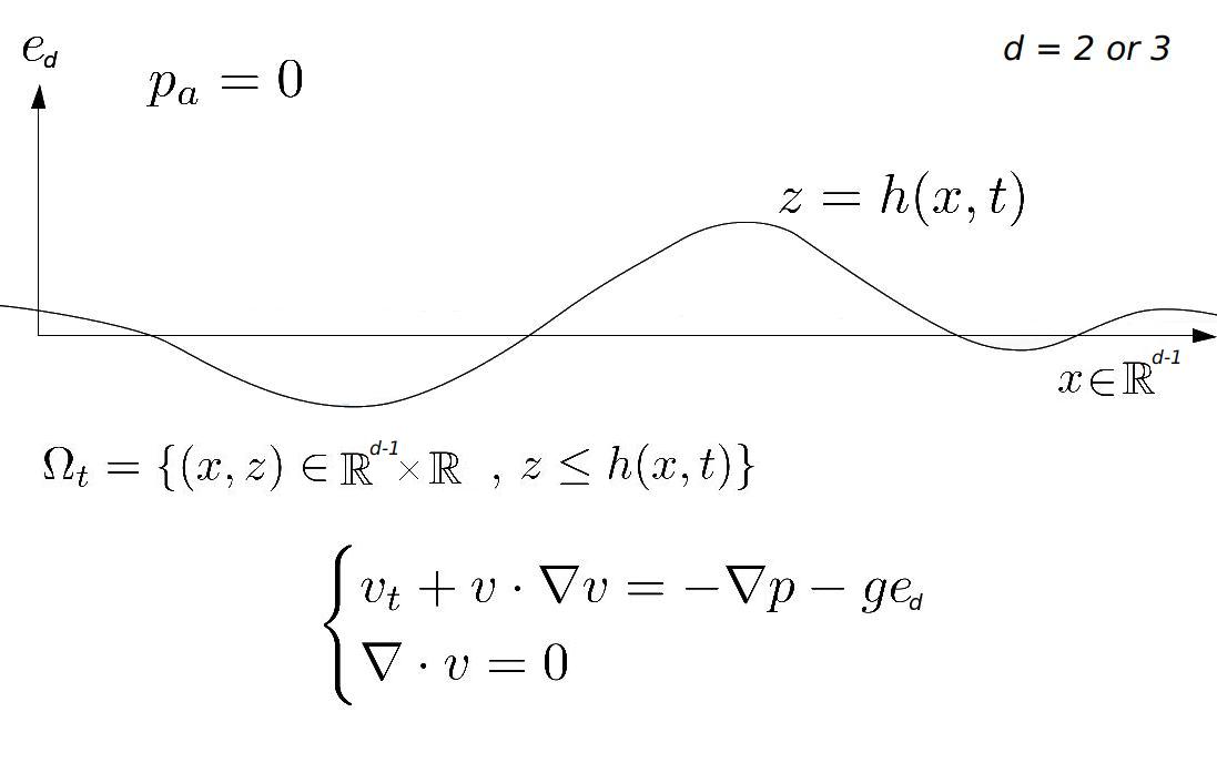
Figure 1. The water waves problem in Eulerian coordinates.

Then, the equations of motion can be reduced to the following system for the unknowns $h,\phi:I_{t}\times{\mathbb{R}}^{n-1}_{x}\rightarrow{\mathbb{R}}$:

$$\left\{\begin{array}[]{l}\partial_{t}h=G(h)\phi,\\ \partial_{t}\phi=-gh+\sigma{\,\mbox{div}\,}\Big{[}\dfrac{\nabla h}{(1+|\nabla h|^{2})^{1/2}}\Big{]}-\dfrac{1}{2}{|\nabla\phi|}^{2}+\dfrac{{\left(G(h)\phi+\nabla h\cdot\nabla\phi\right)}^{2}}{2(1+{|\nabla h|}^{2})}.\end{array}\right.$$ (1.7)

Here

$$G(h):=\sqrt{1+{|\nabla h|}^{2}}\mathcal{N}(h),\qquad\mathcal{N}(h)\phi:=\nabla_{n}\Phi,$$ (1.8)

where $n$ is the outward unit normal to $S_{t}$, and $\mathcal{N}(h)$ denotes the Dirichlet–Neumann map associated to the domain $\Omega_{t}$. Roughly speaking, one can think of $G(h)$ as a first order, non-local, linear operator that depends nonlinearly on the domain. We refer to [131, chap. 11] or the book of Lannes [101] for the derivation of (1.7), which is the so-called Zakharov-Craig-Schanz-Sulem [50] formulation.

The system (1.7) admits the conserved energy

$$\begin{split}\mathcal{H}(h,\phi)&:=\frac{1}{2}\int_{{\mathbb{R}}^{n-1}}G(h)\phi\cdot\phi\,dx+\frac{g}{2}\int_{{\mathbb{R}}^{n-1}}h^{2}\,dx+\sigma\int_{{\mathbb{R}}^{n-1}}\frac{{|\nabla h|}^{2}}{1+\sqrt{1+|\nabla h|^{2}}}\,dx\end{split}$$ (1.9)

which is the sum of the kinetic energy corresponding to the $L^{2}$ norm of the velocity field and the potential energy due to gravity and surface tension. It was first observed by Zakharov [150] that (1.7) is the Hamiltonian flow associated to (1.9). For sufficiently small and smooth solutions one has

$$\begin{split}\mathcal{H}(h,\phi)&\approx{\big{\|}|\nabla|^{1/2}\phi\big{\|}}_{L^{2}}^{2}+{\big{\|}(g-\sigma\Delta)^{1/2}h\big{\|}}_{L^{2}}^{2}.\end{split}$$ (1.10)

The formal linearization of (1.7)-(1.8) around a flat and still interface is

$$\partial_{t}h=|\nabla|\phi,\qquad\partial_{t}\phi=-gh+\sigma\Delta h.$$ (1.11)

By defining the linear dispersion relation

$$\Lambda_{g,\sigma}:=\sqrt{g|\nabla|+\sigma|\nabla|^{3}},$$ (1.12)

the identitites (1.11) can be written as a single equation for a complex-valued unknown,

$$\partial_{t}u+i\Lambda_{g,\sigma}u=0,\qquad u:=\sqrt{g+\sigma|\nabla|^{2}}h+i|\nabla|^{1/2}\phi.$$ (1.13)

One generally refers to (1.7) as the gravity water waves system when $g>0$ and $\sigma=0$, as the capillary water waves system when $g=0$ and $\sigma>0$, and as the gravity-capillary water waves system when $g>0$ and $\sigma>0$.

We remark that the presence of the various forces (gravity and/or surface tension) does have an impact on the existence theory of solutions. In the local existence theory this impact is mostly quantitative and the techniques developed for a specific scenario are likely to be adaptable to others. On the other hand, when considering the long-time existence of solutions, the presence of gravity and/or surface tension has a major impact on the evolution. This can be seen already at the level of the linearized equations (1.13), and is even more apparent when looking at three waves resonant interactions, (quadratic time-resonances), and at fully coherent interactions (space-time resonances). We explain these concepts in Section 3.2.

1.4. Other approaches and formulations

There are of course other possible descriptions of the equations. In the series of works [142]–[146], see also the survey [148], Wu uses a combination of Lagrangian coordinates and tools from complex analysis such as the Riemann mapping Theorem and the theory of holomorphic functions (Clifford analysis in $3$d). Lagrangian coordinates and variations have been used in [104, 32, 42], and complex coordinates in the works of Nalimov [110], in Zakharov et al. [62] in various theoretical and numerical works, see for example [153, 63] and references therein, and in the series of papers [79]-[82].

2. Local well-posedness

Because of the complicated nature of the equations, the development of a basic local wellposedness theory (existence and uniqueness of smooth solutions for the Cauchy problem) has proved to be highly non-trivial. Early results on the local wellposedness of the water waves system include those by Nalimov [110], Shinbrot [122], Yosihara [149], and Craig [45]. All these results deal with small perturbations of a flat interface for which the Rayleigh-Taylor sign condition (1.2) always holds. It was first observed by Wu [143] that, in the irrotational case, (1.2) holds without smallness assumptions, and that local-in-time solutions can be constructed with initial data of arbitrary size in Sobolev spaces [142, 143]. Following the breakthrough of Wu, the question of local wellposedness of the water waves and free boundary Euler equations has been addressed by several authors. Christodoulou–Lindblad [32] and Lindblad [104] considered the problem with vorticity, Beyer–Gunther [24] took into account the effects of surface tension, and Lannes [99] treated the case of non-trivial bottom topography. The works by Ambrose-Masmoudi [12], Coutand–Shkoller [42], and Shatah–Zeng [119] extended these results to more general scenarios with vorticity and surface tension, including two-fluids systems [29, 120, 121] where surface tension is necessary for wellposedness. Other important papers that include surface tension and/or low regularity analysis are those by Christianson–Hur–Staffilani [31], and Alazard–Burq–Zuily [1, 2]. See also [117, 154, 109, 95, 147, 98, 55].

Thanks to all the contributions mentioned above the local well-posedness theory is presently well-understood in a variety of different scenarios. In short, one can say that for sufficiently nice initial configurations, it is possible to find classical smooth solutions on a small time interval. See Theorem 2.3 for a typical result in the case of irrotational flows.

To explain some aspects of the local well-posedness theory we follow the approach in Lannes [99], Alazard–Métivier [7] and the series of works by Alazard–Burq–Zuily [1]-[4], based on the use of paradifferential calculus. We choose this path mostly because it is a good starting point for the long-time regularity theory, which we discuss in the next section.

2.1. Paradifferential analysis

The main objective of the paradifferential analysis of the water waves system is to formulate the Hamiltonian system (1.7)-(1.8) for the unknowns $h$ and $\phi$ in terms of new unknowns $h$ and $\omega$, so that the quasilinear structure of the system is apparent. In other words, one wants to identify the terms that are responsible for the loss of derivatives in the nonlinearity, and write the equations in a convenient form, so that it is possible to obtain a priori energy estimates by a relatively simple procedure. A key point is to achieve a good understanding of the Dirichlet–Neumann operator $G(h)\phi$ in (1.8).

2.1.1. Elements of paradifferential calculus

Given a symbol $a=a(x,\zeta)$, $x,\zeta\in{\mathbb{R}}^{d}$, and a function $f\in L^{2}({\mathbb{R}}^{d})$, we define the paradifferential operator $T_{a}f$ according to

$$\mathcal{F}\big{(}T_{a}f\big{)}(\xi)=\frac{1}{(2\pi)^{d}}\int_{{\mathbb{R}}^{2}}\chi\Big{(}\tfrac{|\xi-\eta|}{|\xi+\eta|}\Big{)}\widetilde{a}\big{(}\xi-\eta,\tfrac{\xi+\eta}{2}\big{)}\widehat{f}(\eta)\,d\eta,$$ (2.1)

where $\widehat{g}$ is the Fourier transform of $g$, $\widetilde{a}$ denotes the Fourier transform of $a$ in the first coordinate and $\chi:[0,\infty)\mapsto[0,1]$ is a smooth function supported in $[0,2^{-20}]$ and equal to $1$ on $[0,2^{-21}]$.

Notice that when $a=a(\zeta)$, (2.1) reduces to a standard Fourier multiplier. If instead $a=a(x)$, then $T_{a}f$ is the product of $a$ and $f$ where the frequencies of $a$ are restricted to have size comparable or smaller than the frequencies of $f$. In particular, $T_{a}f$ has the same regularity of $f$. Moreover, one has the basic paradifferential decomposition of Bony [25]:

$$fg=T_{f}g+T_{g}f+\mbox{smoother terms}.$$

There are various ways to measure symbols $a=a(x,\zeta)$ and the norms of the associated paradifferential operators. Without going into technical details one should think of the homogeneity of $a$ with respect to the variable $\zeta$, when $|\zeta|\geq 1$, as representing the order of the paradifferential operator, i.e., the number of derivatives acting on the function $f$, while the dependence on $x$ is somewhat less relevant as far as regularity is concerned (which is what one cares about to establish local existence). A simple choice of a norm for symbols is

$${\|a\|}_{\mathcal{M}^{l}_{r,q}}:=\sup_{|\alpha|+|\beta|\leq r}\sup_{\zeta\in{\mathbb{R}}^{d}}\,\langle\zeta\rangle^{-l}\|\,|\zeta|^{|\beta|}\partial^{\beta}_{\zeta}\partial_{x}^{\alpha}a\|_{L^{q}_{x}({\mathbb{R}}^{d})},$$ (2.2)

where $l\in{\mathbb{R}}$ is the order of the symbol (and of the associated paradifferential operator), $r\in\mathbb{N}$ measures the smoothness in $x$, and $q\in[1,\infty]$ the integrability.

As in the case of differential operators, it is possible to establish several algebra properties for suitable classes of paradifferential operators. In particular, one has the mapping property

$$a:H^{s}\mapsto H^{s-l},\qquad\mbox{for}\quad\,a\in\mathcal{M}^{l}_{r,\infty},$$ (2.3)

and the formulas

$$T_{a}T_{b}\approx T_{ab},\qquad[T_{a},T_{b}]\approx iT_{\{a,b\}},\qquad(T_{a})^{\ast}=T_{\overline{a}},$$ (2.4)

where $\approx$ denotes an equality up to terms of lower order, $[\cdot,\cdot]$ is the commutator, and $\{a,b\}:=\nabla_{x}a\nabla_{\zeta}b-\nabla_{\zeta}a\nabla_{x}b$ is the Poisson bracket.

2.1.2. The “good unknown” and the Dirichlet-Neumann operator

To describe the action of the Dirichlet-Neumann (DN) operator one introduces

$$B:=\frac{G(h)\phi+\nabla_{x}h\cdot\nabla_{x}\phi}{1+|\nabla h|^{2}},\qquad V:=\nabla_{x}\phi-B\nabla_{x}h,\qquad\omega:=\phi-T_{B}h.$$ (2.5)

Here $(V,B)\in{\mathbb{R}}^{n-1}\times{\mathbb{R}}$ is the restriction to the interface of the velocity field $v$ of the fluid, and function $\omega$ is the so-called “good-unknown” of Alinhac [8, 9, 7]. The origin of $\omega$ is in the paracomposition formula $f\circ g\approx T_{f^{\prime}\circ g}g$, which holds when $g$ is rougher than $f$. As a result, the variable $\omega$ in (2.5) has better smoothness properties than $\phi$, when $h$ has limited regularity. One of the most important outcomes of the paradifferential analysis in the context of water waves is the following key formula for the DN operator:

Proposition 2.1 (Paralinearization of the DN operator).

Let $G(h)$ be the operator defined in (1.8), with (1.5)-(1.6), and let $\omega,B,V$ be given by (2.5). Then we have

$$G(h)\phi=T_{\lambda_{DN}}\omega-{\,\mbox{div}\,}(T_{V}h)+G_{2},$$ (2.6)

where $G_{2}$ denotes smoother terms which are also quadratic in the unknowns, and the symbol of the operator is given by

$$\begin{split}\lambda_{DN}&:=\lambda^{(1)}+\lambda^{(0)},\\ \lambda^{(1)}(x,\zeta)&:=\sqrt{(1+|\nabla h|^{2})|\zeta|^{2}-(\zeta\cdot\nabla h)^{2}},\\ \lambda^{(0)}(x,\zeta)&:=\Big{(}\frac{(1+|\nabla h|^{2})^{2}}{2\lambda^{(1)}}\Big{\{}\frac{\lambda^{(1)}}{1+|\nabla h|^{2}},\frac{\zeta\cdot\nabla h}{1+|\nabla h|^{2}}\Big{\}}+\frac{1}{2}\Delta h\Big{)}.\end{split}$$ (2.7)

This proposition shows the relevance of the good unknown in the fact that the main action of the DN map can be expressed in terms of a paradifferential operator acting on $\omega$, plus a simple transport-like term ${\,\mbox{div}\,}(T_{V}h)$.

2.1.3. Diagonalization and energy estimates

Using (2.6) and standard paralinearization arguments, one can reduce (1.7) to the following system:

$$\left\{\begin{array}[]{l}\partial_{t}h=T_{\lambda_{DN}}\omega-{\,\mbox{div}\,}(T_{V}h)+G_{2}\\ \\ \partial_{t}\omega=-gh-T_{\ell}h-T_{V}\nabla\omega+\Omega_{2}\end{array}\right.$$ (2.11)

where

$$\begin{split}\ell(x,\zeta)&:=L_{ij}(x)\zeta_{i}\zeta_{j}-(g|\nabla|+\sigma|\nabla|^{3})h,\qquad L_{ij}:=\frac{\sigma}{\sqrt{1+|\nabla h|^{2}}}\Big{(}\delta_{ij}-\frac{\partial_{i}h\partial_{j}h}{1+|\nabla h|^{2}}\Big{)},\end{split}$$ (2.12)

and $G_{2}$ and $\Omega_{2}$ denote smoother terms which are quadratic in the unknowns. One can then arrive at the following result:

Proposition 2.2 (Diagonalization and a priori energy estimates).

Let $(h,\omega)$ be solutions of (2.11)-(2.12), and recall the notation (2.1) and (2.5). Define the diagonal variable

$$U:=T_{\sqrt{g+\ell}}h+iT_{\Sigma}T_{1/\sqrt{g+\ell}}\omega,$$ (2.13)

where

$$\Sigma :=\sqrt{\lambda_{DN}(g+\ell)}$$ (2.14)

is the diagonal symbol. Then, the following hold:

• $U$ satisfies the equation

  $$\begin{split}&\partial_{t}U+iT_{\Sigma}U+iT_{V\cdot\zeta}U=\mathcal{N}_{U}\end{split}$$ (2.15)

  where $\mathcal{N}_{U}$ denotes nonlinear terms of lower order.

• For any $k\geq 0$ consider

  $$E(t):=\int_{{\mathbb{R}}^{d}}\big{|}W(t,x)\big{|}^{2}\,dx,\qquad W:=T_{\Sigma}^{k}U;$$ (2.16)

  then

  $$E(t)\sim{\|U(t)\|}_{H^{3k/2}}^{2}\qquad\mbox{and}\qquad\frac{d}{dt}E(t)\lesssim P\big{(}E(t)\big{)}\,E(t),$$ (2.17)

  where $P$ is a polynomial with positive coefficients.

The procedure leading to (2.15) is the nonlinear analogue of the basic diagonalization in (1.13). For the purpose of the local existence theory one can think of the nonlinear terms having the form $\mathcal{N}_{U}=U^{2}$. Then, the paralinearized equation (2.15) has a fairly simple structure which allows one to derive the energy estimates (2.17) in a relatively straightforward fashion, for example by applying multiple times the operator $T_{\Sigma}$. (2.17) gives a priori control on a short time interval on the function $U$ in the space $H^{3k/2}$, and hence control on $(g-\sigma\Delta)h$ and $|\nabla|^{1/2}\phi$ in the same space. Once these a priori estimates are established, local well-posedness can then be obtained by standard procedures. In conclusion one obtains the following result:

Theorem 2.3 (Local well-posedness of (1.7)).

Consider the system of equations (1.7). Let an intial data $h_{0}=h(t=0)$, $\phi_{0}=\phi(t=0)$, be given so that with $\sqrt{g-\sigma\Delta}\,h_{0}$, $|\nabla|^{1/2}\phi\in H^{s}$, for $s>\tfrac{d}{2}+1$ large enough. Then, there exists $T>0$ and a unique solution

$$\big{(}\sqrt{g-\sigma\Delta}\,h,|\nabla|^{1/2}\phi\big{)}\in C\big{(}[-T,T],H^{s}\times H^{s}\big{)}$$

of the system (1.7) with the assigned initial data.

We notice that, at the linear level,

$$\Sigma\approx\sqrt{g|\nabla|+\sigma|\nabla|^{3}}=:\Lambda_{g,\sigma}(\nabla),\qquad U\approx\sqrt{g-\sigma\Delta}\,h+i|\nabla|^{1/2}\omega.$$ (2.18)

This is used to construct suitable models for global analysis, see (3.4)–(3.5) and (3.33).

2.2. Conclusion

We have summarized the main ingredients in the local existence theory using Eulerian coordinates. This is a natural description, which is also tied to the Hamiltonian nature of the equations, and is a good starting point for the global theory. The other formulations described in subsection 1.4 can also be used to develop the local theory, as in the references mentioned at the beginning of the section. This includes, of course, well-posedness results in the presence of vorticity analogous to Theorem 2.3. We also refer to recent work of Lannes on the interaction with floating structures [102] and de Poyferré [54] on emerging bottom.

3. Global regularity and asymptotic behavior

The problem of global existence of solutions for water waves models is more challenging, and much fewer results have been obtained so far. As in many other quasilinear problems, global regularity has been studied in a perturbative and dispersive setting. Large initial data can lead to breakdown in finite time, see for example the papers on “splash” singularities [27, 43].

In three dimensions (2D interfaces), the first global regularity results were proved by Germain-Masmoudi-Shatah [70] and Wu [146] for the gravity problem ($g>0$, $\sigma=0$). Global regularity in $3$D was also proved for the capillary problem ($g=0$, $\sigma>0$) by Germain-Masmoudi-Shatah [71] and for the full gravity-capillary problem ($g>0$, $\sigma>0$) by Deng-Ionescu-Pausader-Pusateri [60]. In the case of a finite flat bottom, global regularity was proved recently by Wang [137, 138, 139] in both the gravity and the capillary problems in $3$D.

In two dimensions (1D interfaces), the first long-time result for the water waves system (1.7) is due to Wu [145], who showed almost-global existence for the gravity problem ($g>0$, $\sigma=0$). This was improved to global regularity by the authors in [87] and, independently, by Alazard-Delort [5, 6]. A different proof of Wu’s $2$D almost global existence result was later given by Hunter-Ifrim-Tataru [79], and then complemented to a proof of global regularity in [80]. See also Wang [136] for a global regularity result for a class of small data of infinite energy. For the capillary problem in $2$D, global regularity was proved by the authors in [89] and, independently, by Ifrim-Tataru [81] in the case of data satisfying an additional momentum condition.

We remark that all the global regularity results that have been proved so far require 3 basic assumptions: small data (small perturbations of the rest solution), trivial vorticity inside the fluid, and flat Euclidean geometry. More subtle properties are also important, such as the Hamiltonian structure of the equations, the rate of decay of the linearized waves, and the resonance structure of the bilinear wave interactions.

3.1. Main ideas

The classical mechanism to establish global regularity for quasilinear equations has two main components:

• Propagate control of high order energy functionals (Sobolev norms and weighted norms);

• Prove dispersion and decay of the solution over time.

The interplay of these two aspects has been present since the seminal work of Klainerman [96, 97] on nonlinear wave equations and vector-fields, Shatah [118] on $3$d Klein-Gordon and normal forms, Christodoulou-Klainerman [33] on the stability of Minkowski space-time, and Delort [57] on $1$d Klein-Gordon equations.

In the last few years new methods have emerged in the study of global solutions of quasilinear evolutions, inspired by the advances in semilinear theory. The basic idea is to combine the classical energy and vector-fields methods with refined analysis of the Duhamel formula, using the Fourier transform and carefully constructed “designer norms”. This is the essence of the “method of space-time resonances” of Germain-Masmoudi-Shatah [70, 71, 69] and Gustafson-Nakanishi-Tsai [74], and of the work on plasma models and water waves in [84, 85, 73, 59, 86, 87, 88, 89, 60].

In the rest of this section we illustrate the development of the these ideas in the setting of water waves by analyzing 3 systems, in increasing order of difficulty: gravity water waves in 3D, gravity water waves in 2D, and gravity-capillary water waves in 3D.

For the sake of exposition, in all three cases we take the following approach: we replace the full water waves systems with suitable simplified quasilinear models, and then outline the main ideas needed to analyze these models. The quasilinear models constructed here have two main properties: (1) they capture the essential difficulties of the global theory of the full systems, and (2) they are technically simpler than the full systems, mainly because they bypass all the difficulties of the local theory, such as the use of paradifferential calculus.

One should keep in mind that there are certain difficulties in transferring the global analysis from the model equations to the real water waves systems, mostly at the level of the energy estimates. Nevertheless, our simplified models are very useful to explain some of the key ideas of the global analysis, in problems that are more algebraically transparent.

3.2. Gravity water waves in 3D

We consider first the system (1.7) in 2D in the case $(g,\sigma)=(1,0)$. Global regularity in this case was proved in [70] and [146]. Here we follow essentially the exposition and the proof of Germain-Masmoudi-Shatah [70]; Wu’s theorem in [146] is essentially equivalent, but involves slightly different hypothesis on the data and a very different proof (in Lagrangian coordinates, using also the Clifford algebra).

Theorem 3.1.

Assume that $h_{0},\phi_{0}:\mathbb{R}^{2}\to\mathbb{R}$ are small and smooth initial data, satisfying

$$\|U_{0}\|_{H^{N+1}}+\sum_{l\in\{1,2\}}\|\,|\nabla|^{1-p}(x_{l}U_{0})\|_{L^{2}}+\sup_{t\in[0,\infty)}\langle t\rangle\|e^{-it\Lambda}U_{0}\|_{W^{4,\infty}}\leq{\varepsilon}\leq\overline{{\varepsilon}}$$ (3.1)

where $N$ is sufficiently large, $\overline{{\varepsilon}}$ is sufficiently small, $p=1/4$, $\langle t\rangle^{-1}=\sqrt{1+t^{2}}$, and

$$U_{0}:=h_{0}+i|\nabla|^{1/2}\phi_{0},\qquad\Lambda:=\Lambda_{1,0}=\sqrt{|\nabla|}.$$ (3.2)

Then there is a unique global solution $U=h+i|\nabla|^{1/2}\phi\in C([0,\infty):H^{N}(\mathbb{R}^{2}))$ of the initial-value problem (1.7) with $(g,\sigma)=(1,0)$. Moreover the solution satisfies the global bounds

$$\langle t\rangle^{-\delta}\|U(t)\|_{H^{N}}+\langle t\rangle^{-\delta}\|\,|\nabla|^{1-p}(x_{l}u(t))\|_{L^{2}}+\langle t\rangle\|U(t)\|_{W^{4,\infty}}+\|U(t)\|_{L^{2}}\lesssim{\varepsilon},$$ (3.3)

for any $t\in[0,\infty)$ and $l\in\{1,2\}$, where $\delta=10^{-8}$ is a small constant and $u(t):=e^{it\Lambda}U(t)$ is the associated linear profile of the solution $U$.

We describe now some of the main ingredients of the proof. We highlight two main ideas: (1) the proof of high order energy estimates by symmetrization, and (2) the proof of dispersive estimates using the method of space-time resonances.

To simplify the exposition we replace the system (1.7) with the quasilinear evolution equation

$$(\partial_{t}+i\Lambda)U=\mathcal{N}.$$ (3.4)

The quadratic nonlinearity $\mathcal{N}$ is defined by

$$\widehat{\mathcal{N}}(\xi):=\frac{1}{(2\pi)^{2}}\int_{\mathbb{R}^{2}}\varphi_{[-10,10]}(|\eta|/|\xi|)\sum_{l\in\{1,2\}}\widehat{V_{l}}(\xi-\eta)\widehat{\partial_{l}U}(\eta)\,d\eta,\qquad V:=\nabla(|\nabla|^{-1/2}\Re U).$$ (3.5)

Here, and in the rest of the section, we use smooth cutoff functions defined as follows: we fix an even smooth function $\varphi:{\mathbb{R}}\to[0,1]$ supported in $[-2,2]$ and equal to $1$ in $[-1,1]$, and let

$$\varphi_{k}(x):=\varphi(x/2^{k})-\varphi(x/2^{k-1}),\qquad\varphi_{I}(x):=\sum_{k\in\mathbb{I}}\varphi_{k}(x),$$

for any $k\in\mathbb{Z}$ and interval $I\subseteq\mathbb{R}$. We define also the Littlewood-Paley projections $P_{k}$, $P_{I}$ as the operators induced by the Fourier multipliers $\varphi_{k}$, and $\varphi_{I}$ respectively. The equations (3.4)–(3.5) are a good substitute for the full system (1.7), see the discussion in section 2.

The proof relies on a bootstrap argument: we assume that $U\in C([0,T]:H^{N}(\mathbb{R}^{2}))$ is a solution of (3.4)–(3.5) satisfying the bootstrap hypothesis

$$\langle t\rangle^{-\delta}\|U(t)\|_{H^{N}}+\langle t\rangle^{-\delta}\sum_{l\in\{1,2\}}\|\,|\nabla|^{1-p}(x_{l}u(t))\|_{L^{2}}+\langle t\rangle\|U(t)\|_{W^{4,\infty}}+\|U(t)\|_{L^{2}}\leq{\varepsilon}_{1},$$ (3.6)

for any $t\in[0,T]$, where ${\varepsilon}_{1}:={\varepsilon}^{2/3}$, and we would like to prove the improved bounds

$$\langle t\rangle^{-\delta}\|U(t)\|_{H^{N}}+\langle t\rangle^{-\delta}\sum_{l\in\{1,2\}}\|\,|\nabla|^{1-p}(x_{l}u(t))\|_{L^{2}}+\langle t\rangle\|U(t)\|_{W^{4,\infty}}+\|U(t)\|_{L^{2}}\lesssim{\varepsilon}.$$ (3.7)

This suffices, by a simple continuity argument, since the stronger bounds (3.7) hold at time $t=0$ due to the initial-data assumptions (3.1).

We remark that the bootstrap norms used in (3.6) capture the main features of the nonlinear solution, namely smoothness, localization in space, and sharp pointwise decay matching the decay of linear gravity waves.

3.2.1. Energy estimates

These are very simple in our model (3.4)–(3.5): we define

$$W=W_{N}:=\langle\nabla\rangle^{N}U,\qquad\mathcal{E}_{N}(t):=\|\langle\nabla\rangle^{N}U(t)\|_{L^{2}}^{2}=\frac{1}{(2\pi)^{2}}\int_{\mathbb{R}^{2}}|\widehat{W}(\xi)|^{2}\,d\xi.$$ (3.8)

Then we calculate, using the equation and symmetrization (or integration by parts)

$$\frac{d}{dt}\mathcal{E}_{N}=C\int_{\mathbb{R}^{2}\times\mathbb{R}^{2}}\widehat{W}(\eta)\overline{\widehat{W}(\xi)}\widehat{\Re U}(\xi-\eta)m(\xi,\eta)\,d\xi d\eta,$$ (3.9)

where

$$m(\xi,\eta)=\frac{\langle\xi\rangle^{N}}{\langle\eta\rangle^{N}}\frac{(\xi-\eta)\cdot\eta}{|\xi-\eta|^{1/2}}\varphi_{[-10,10]}(|\eta|/|\xi|)-\frac{\langle\eta\rangle^{N}}{\langle\xi\rangle^{N}}\frac{(\xi-\eta)\cdot\xi}{|\xi-\eta|^{1/2}}\varphi_{[-10,10]}(|\xi|/|\eta|).$$ (3.10)

The symmetrization in the symbol $m$ avoids the potential loss of derivative, and the identity above can be easily used to show that

$$\big{|}\mathcal{E}_{N}(t)-\mathcal{E}_{N}(0)\big{|}\lesssim\int_{0}^{t}\mathcal{E}_{N}(s)\cdot\|U(s)\|_{W^{4,\infty}}\,ds.$$ (3.11)

This leads to the desired improved energy bound in (3.7). Notice how this step relies in a crucial way on the sharp pointwise decay of $\langle t\rangle^{-1}$ for $U(t)$.

We remark that in the real water waves systems analyzed in [70] and [146] the final result is similar (an energy inequality similar to (3.11)), but the proof is substantially more complicated because of the quasilinear structure of the problem. In particular, the proof has to address all the difficulties of the local regularity theory of the water waves models.

3.2.2. Dispersion and decay

It remains to control the other terms in (3.7). The idea is to write the equation in terms of the linear profile $u(t):=e^{it\Lambda}U(t)$,

$$\partial_{t}\widehat{u}(\xi,t)=\sum_{+,-}\int_{\mathbb{R}^{2}}e^{it[\Lambda(\xi)\mp\Lambda(\xi-\eta)\mp\Lambda(\eta)]}m_{\pm\pm}(\xi,\eta)\widehat{u_{\pm}}(\xi-\eta,t)\widehat{u_{\pm}}(\eta,t)\,d\eta,$$ (3.12)

where $u_{+}:=u$, $u_{-}:=\overline{u}$, the sum is taken over choices of the signs $+,-$, and $m_{\pm\pm}$ are suitable smooth multipliers. In integral form this becomes

$$\widehat{u}(\xi,t)=\widehat{u}(\xi,0)+\sum_{+,-}\int_{0}^{t}\int_{\mathbb{R}^{2}}e^{is[\Lambda(\xi)\mp\Lambda(\xi-\eta)\mp\Lambda(\eta)]}m_{\pm\pm}(\xi,\eta)\widehat{u_{\pm}}(\xi-\eta,s)\widehat{u_{\pm}}(\eta,s)\,d\eta ds.$$ (3.13)

One would like to estimate $u$ by integrating by parts either in $s$ or in $\eta$. According to [70], the main contribution is expected to come from the set of quadratic space-time resonances (the stationary points of the integral)

$$\mathcal{SR}:=\{(\xi,\eta):\,\Phi(\xi,\eta)=0,\,(\nabla_{\eta}\Phi)(\xi,\eta)=0,\,m(\xi,\eta)\neq 0\},$$ (3.14)

where $m=m_{\pm\pm}$ and the phases $\Phi$ are defined by

$$\Phi(\xi,\eta):=\Lambda(\xi)\mp\Lambda(\xi-\eta)\mp\Lambda(\eta).$$ (3.15)

Since $\Lambda(\rho)=\sqrt{|\rho|}$, the first main observation is that the phases $\Phi$ only vanish when either $\xi=0$, or $\eta=0$, or $\xi-\eta=0$. In this case, however, the multipliers $m$ also vanish. In other words, there are no quadratic time resonances and one can use normal forms (integration by parts in time) to transform the quadratic terms into cubic terms.

Loss of derivative is not important at this stage of the argument, so one can integrate by parts in time and use (3.12). It remains to estimate the contribution of cubic terms of the form

$$\int_{0}^{t}\int_{\mathbb{R}^{2}\times\mathbb{R}^{2}}e^{is\widetilde{\Phi}(\xi,\eta,\sigma)}\frac{m(\xi,\eta)}{\Phi(\xi,\eta)}m^{\prime}(\eta,\sigma)\widehat{u_{\pm}}(\xi-\eta,s)\widehat{u_{\pm}}(\eta-\sigma,s)\widehat{u_{\pm}}(\sigma,s)\,d\eta d\sigma ds,$$ (3.16)

where $\widetilde{\Phi}(\xi,\eta,\sigma):=\Lambda(\xi)\mp\Lambda(\xi-\eta)\mp\Lambda(\eta-\sigma)\mp\Lambda(\sigma)$.

The resulting multiplier $\frac{m(\xi,\eta)}{\Phi(\xi,\eta)}m^{\prime}(\eta,\sigma)$ is regular, so one can now analyze cubic integrals of this type using again the method of space-time resonances. An important algebraic observation, which is used in the analysis of the phases $\widetilde{\Phi}_{--+},\widetilde{\Phi}_{-+-},\widetilde{\Phi}_{+--}$ to control the weighted norms, is the identity

$$\nabla_{\xi}\widetilde{\Phi}(\xi,\eta,\sigma)=0\quad\text{ if }\quad\nabla_{\eta,\sigma}\widetilde{\Phi}(\xi,\eta,\sigma)=0\quad\text{ and }\quad|\eta|,|\xi-\sigma|\ll|\xi|.$$ (3.17)

This is a slow propagation of iterated resonances property; more subtle versions of this property are also important in the 3D gravity-capillary model described below, see for example (3.53).

The dispersive analysis in [70] is simplified by the fact that there are no quadratic space-time resonances in the problem. However, the basic idea of the method of space-time resonances, namely to identify these points and center the analysis around them, plays a crucial role in many other global regularity results on plasma models and water waves models. Further developments of these ideas, and much more sophisticated arguments, are used in the proof global regularity for the 3D gravity-capillary model, where one has to deal with a full set of quadratic space-time resonances. See subsection 3.4.

3.3. Gravity water waves in 2D

We consider now the system (1.7) in 1D in the case $(g,\sigma)=(1,0)$. Global regularity in this case was proved in [145, 87, 5, 6, 79, 80, 136]. The precise assumptions on the initial data (low frequencies, high frequencies, and the number of vector-fields involved) are not identical in these papers. We will follow mostly the setup in [87].

Theorem 3.2.

Assume that $h_{0},\phi_{0}:\mathbb{R}\to\mathbb{R}$ are small and smooth initial data, satisfying

$$\|U_{0}\|_{H^{N+2}}+\|x\partial_{x}U_{0}\|_{H^{N/2+1}}+\|U_{0}\|_{Z}\leq{\varepsilon}\leq\overline{{\varepsilon}}$$ (3.18)

where $N$ is sufficiently large, $\overline{{\varepsilon}}$ is a sufficiently small constant, $U_{0}=h_{0}+i|\nabla|^{1/2}\phi_{0}$, and

$$\|f\|_{Z}:=\big{\|}(|\xi|^{\beta}+|\xi|^{N/2+10})\widehat{f}(\xi)\big{\|}_{L^{\infty}_{\xi}},\qquad\beta:=1/4.$$ (3.19)

(i) Then there is a unique global solution $U=h+i|\nabla|^{1/2}\phi\in C([0,\infty):H^{N}(\mathbb{R}))$ of the initial-value problem (1.7) with $(g,\sigma)=(1,0)$. The solution $U$ satisfies the global bounds

$$\langle t\rangle^{-\delta}\|U(t)\|_{H^{N}}+\langle t\rangle^{-\delta}\|SU(t)\|_{H^{N/2}}+\langle t\rangle^{1/2}\|U(t)\|_{W^{N/2+4,\infty}}\lesssim{\varepsilon},$$ (3.20)

for any $t\in[0,\infty)$, where $S:=(1/2)t\partial_{t}+x\partial_{x}$ is the scaling vector-field and $\delta=10^{-8}$ is small.

(ii) The solution $U(t)$ undergoes modified (nonlinear) scattering as $t\to\infty$, i.e.

$$\lim_{t\to\infty}\mathcal{F}^{-1}\{e^{iG(\xi,t)}e^{it\Lambda(\xi)}\widehat{U}(\xi,t)\}=u^{\ast}_{\infty}\text{ in }H^{N/2}$$ (3.21)

where $\Lambda(\xi)=\sqrt{|\xi|}$ and

$$G(\xi,t):=\frac{|\xi|^{4}}{\pi}\int_{0}^{t}|\widehat{U}(\xi,s)|^{2}\frac{ds}{s+1}.$$ (3.22)

As before, we discuss two main ideas of the proof: (1) the quartic energy inequality which is needed to prove energy estimates, and (2) the construction of nonlinear profiles, to prove modified scattering and dispersion. As before, we use the simplified model

$$\begin{split}&(\partial_{t}+i\Lambda)U=\mathcal{N},\\ &\widehat{\mathcal{N}}(\xi):=\frac{1}{2\pi}\int_{\mathbb{R}}\varphi_{[-10,10]}(|\eta|/|\xi|)\widehat{V}(\xi-\eta)\widehat{\partial_{x}U}(\eta)\,d\eta,\qquad V:=\partial_{x}(|\nabla|^{-1/2}\Re U),\end{split}$$ (3.23)

which is the $1D$ analogue of the model (3.4)–(3.5). We use again a bootstrap argument, with the bootstrap hypothesis

$$\langle t\rangle^{-\delta}\|U(t)\|_{H^{N}}+\langle t\rangle^{-\delta}\|SU(t)\|_{H^{N/2}}+\langle t\rangle^{1/2}\|U(t)\|_{W^{N/2+4,\infty}}\leq{\varepsilon}_{1}={\varepsilon}_{0}^{2/3},$$ (3.24)

for a solution on some time interval $[0,T]$.

3.3.1. Energy estimates

One can start proving energy estimates as in the 2D model, see (3.8)–(3.11). These identities still hold, but the bound (3.11) does not suffice to close the energy estimate, since the optimal $L^{\infty}$-type decay is $\langle t\rangle^{-1/2}$ in 1D, which is far from integrable.

The idea, which was introduced by Wu [145], is to refine the energy method by proving instead a quartic energy inequality of the form

$$\big{|}\mathcal{E}^{\prime}_{N}(t)-\mathcal{E}^{\prime}_{N}(0)\big{|}\lesssim\int_{0}^{t}\mathcal{E}_{N}(s)\cdot\|U(s)\|^{2}_{W^{N/2+4,\infty}}\,ds,$$ (3.25)

for a suitable functional $\mathcal{E}^{\prime}_{N}(t)$ satisfying $\mathcal{E}^{\prime}_{N}(t)\approx\mathcal{E}_{N}(t)\approx\|U(t)\|_{H^{N}}^{2}$. The point is to get two factors of $\|U(s)\|^{2}_{W^{N/2+4,\infty}}$ in the right-hand side, in order to have almost integrable decay.

In our model (3.23), a quartic energy inequality can be proved easily using the identities (3.9)–(3.10). The idea is to write the bulk integrals in the right-hand side of (3.10) in terms of the linear profiles $u=e^{it\Lambda}U$ and $w=e^{it\Lambda}W$ and integrate by parts in time. More precisely, the bulk term can be written as a linear combination of integrals of the form

$$\int_{0}^{t}\int_{\mathbb{R}\times\mathbb{R}}e^{-is(\Lambda(\eta)-\Lambda(\xi)\pm\Lambda(\xi-\eta))}\widehat{w}(\eta,s)\overline{\widehat{w}(\xi,s)}\widehat{u_{\pm}}(\xi-\eta,s)m(\xi,\eta)\,d\xi d\eta,$$ (3.26)

where $m$ is the multiplier defined in (3.10). The key observation is that the phases $\Lambda(\eta)-\Lambda(\xi)\pm\Lambda(\xi-\eta)$ do not vanish, except when one of the frequencies vanishes. In this case, however, the multipliers $m$ vanish as well.

The profiles $w$ satisfy transport equations similar to (3.12). Integration by parts in time and changes of variables show that the integrals in (3.26) can be written as (1) sums of cubic boundary terms of the form

$$\int_{\mathbb{R}\times\mathbb{R}}e^{-is(\Lambda(\eta)-\Lambda(\xi)\pm\Lambda(\xi-\eta))}\widehat{w}(\eta,s)\overline{\widehat{w}(\xi,s)}\widehat{u_{\pm}}(\xi-\eta,s)\frac{m(\xi,\eta)}{\Lambda(\eta)-\Lambda(\xi)\pm\Lambda(\xi-\eta)}\,d\xi d\eta,$$ (3.27)

where $s\in\{0,t\}$, and (2) sums of quartic space-time integrals of the form

$$\begin{split}\int_{0}^{t}\int_{\mathbb{R}\times\mathbb{R}}&e^{-is(\pm\Lambda(-\xi)\pm\Lambda(\sigma)\pm\Lambda(\xi-\eta)\pm\Lambda(\eta-\sigma))}\widehat{w_{\pm}}(-\xi,s)\widehat{w_{\pm}}(\xi,s)\\ &\widehat{u_{\pm}}(\xi-\eta,s)\widehat{u_{\pm}}(\eta-\sigma,s)\widetilde{m}(\xi,\eta,\sigma)\,d\xi d\eta d\sigma.\end{split}$$ (3.28)

All the quartic space-time integrals contain two copies of $w$, two copies of $u$, and, most importantly, the multipliers $\widetilde{m}$ are regular and do not lose high-order derivatives (after suitable symmetrization). The desired inequality (3.25) follows: the boundary cubic expressions in (3.27) can be combined with the quadratic energies $\mathcal{E}_{N}$ to produce the energy functionals $\mathcal{E}^{\prime}_{N}$, while the quartic space-time integrals can be estimated as claimed.

The vector-field norm can also be controlled in a similar way, by proving a similar quartic energy inequality of the form

$$\big{|}\mathcal{E}^{\prime}_{S}(t)-\mathcal{E}^{\prime}_{S}(0)\big{|}\lesssim\int_{0}^{t}(\mathcal{E}_{S}(s)+\mathcal{E}_{N}(s))\cdot\|U(s)\|^{2}_{W^{N/2+4,\infty}}\,ds,$$ (3.29)

for a suitable functional $\mathcal{E}^{\prime}_{S}(t)$ satisfying $\mathcal{E}^{\prime}_{S}(t)\approx\mathcal{E}_{S}(t)\approx\|SU(t)\|_{H^{N/2}}^{2}$.

Quartic energy inequalities such as (3.25) were proved and played a key role in all the (almost) global regularity results for water waves in 2D. As explained above, the main ingredient for such an inequality to hold is the absence of bilinear time-resonances. However, the implementation is somewhat delicate in certain quasilinear problems, like water waves models, due to the potential loss of derivatives. It can be done in some cases, for example either by using carefully constructed nonlinear changes of variables (as in Wu [145], see also [87]), or the “iterated energy method” of Germain–Masmoudi [69], or the “paradifferential normal form method” of Alazard–Delort [6], or the “modified energy method” of Hunter–Ifrim–Tataru [79]. These methods are largely interchangeable, as long as there are no significant quadratic resonances. See also [58] and [78] for earlier constructions proving quartic energy inequalities like (3.25) in simpler models.

The calculation we present above, using integration by parts in time in Fourier variables, has similarities with the I-method of Colliander–Keel–Staffilani–Takaoka–Tao [34, 35], which is used extensively in semilinear problems. One should also compare this with the more involved calculation used in energy estimates in the 3D gravity–capillary model described below.

3.3.2. Modified scattering and decay

One can start again, as in the 2D case, from identities on the profile similar to (3.12)–(3.13). The phases $\Phi(\xi,\eta)=\sqrt{|\xi|}\mp\sqrt{|\eta|}\mp\sqrt{|\xi-\eta|}$ do not vanish (except when one of the frequencies vanishes), so one can use again a normal form. As in (3.16) we have an identity of the type

$$\partial_{t}\widehat{u^{\prime}}(\xi,t)=\sum_{+,-}\int_{\mathbb{R}\times\mathbb{R}}e^{it\widetilde{\Phi}(\xi,\eta,\sigma)}\widetilde{m}(\xi,\eta,\sigma)\widehat{u^{\prime}_{\pm}}(\xi-\eta,t)\widehat{u^{\prime}_{\pm}}(\eta-\sigma,t)\widehat{u^{\prime}_{\pm}}(\sigma,t)\,d\eta d\sigma+\widehat{\mathcal{R}_{\geq 4}}(\xi,t),$$ (3.30)

where $\widetilde{\Phi}_{\pm\pm\pm}(\xi,\eta,\sigma):=\Lambda(\xi)\mp\Lambda(\xi-\eta)\mp\Lambda(\eta-\sigma)\mp\Lambda(\sigma)$, $\widetilde{m}$ are regular multipliers, $u^{\prime}$ is a suitable quadratic modification of $u$, and $\mathcal{R}_{\geq 4}$ is a quartic and higher order remainder.

The situation is different in dimension 1, compared to the dimension $d=2$ analyzed earlier, because of the slow rate of decay of solutions. In fact, it turns out that some of the terms in the right-hand side, which correspond to the cubic space-time resonances, cannot be integrated in time. These cubic space-time resonances appear only in the phases $\Phi_{++-}$, $\Phi_{+-+}$, $\Phi_{-++}$, and correspond to the frequencies $(\xi,\xi,-\xi)$, $(\xi,\xi,-\xi)$, and $(\xi,-\xi,\xi)$ respectively. To remove the non-integrable contribution one can define the nonlinear profiles $u^{\ast}(t)$ by

$$\widehat{u^{\ast}}(\xi,t):=e^{iL(\xi,t)}\widehat{u^{\prime}}(\xi,t),\qquad L(\xi,t):=C|\xi|^{4}\int_{0}^{t}|\widehat{u^{\prime}}(\xi,s)|^{2}\frac{ds}{s+1},$$

where $C$ is a suitable real constant. Using (3.30), one can now show that the renormalized profile $u^{\ast}(t)$ stays bounded and converges (quantitatively) in the $Z$ norm as $t\to\infty$,

$$\|u^{\ast}(t_{2})-u^{\ast}(t_{1})\|_{Z}\lesssim 2^{-\delta m}$$

if $m\geq 0$ and $t_{1}\leq t_{2}\in[2^{m-1},2^{m+1}]$. This leads to global control of the solution and modified scattering, as claimed.

The idea of using nonlinear profiles and modified scattering to prove global regularity was introduced in the context of water waves by the authors in [87] and Alazard-Delort in [5, 6]. Just like the quartic energy inequality described earlier, this idea played a key role in all the global regularity results for water waves in 2D.

3.4. Gravity-capillary water waves in 3D

Finally, we consider the system (1.7) in 2D with $(g,\sigma)=(1,1)$, which was analyzed in [60]. Let $\Omega:=x_{1}\partial_{2}-x_{2}\partial_{1}$ denote the rotation vector-field on $\mathbb{R}^{2}$ and let $H^{a,b}_{\Omega}$ denote the space of functions defined by the norm

$$\|f\|_{H^{a,b}_{\Omega}}:=\sum_{j\leq a}\|\Omega^{j}f\|_{H^{b}}.$$

The main result in [60] is the following global regularity theorem:

Theorem 3.3.

Assume that $\delta$ is sufficiently small, $N_{0},N_{1},N_{3}$ are sufficiently large and that the data $(h_{0},\phi_{0})$ satisfies

$$\|U_{0}\|_{H^{N_{0}}\cap H_{\Omega}^{N_{1},N_{3}}}+\|U_{0}\|_{Z}={\varepsilon}\leq\overline{{\varepsilon}},\qquad U_{0}:=(1-\Delta)^{1/2}h_{0}+i|\nabla|^{1/2}\phi_{0},$$ (3.31)

where $\overline{{\varepsilon}}$ is a sufficiently small constant and the $Z$ norm is explained below in 3.4.2, see (3.50). Then, there is a unique global solution $U=(1-\Delta)^{1/2}h+i|\nabla|^{1/2}\phi\in C\big{(}[0,\infty):H^{N_{0}}\big{)}$ of the system (1.7) , with $(h(0),\phi(0))=(h_{0},\phi_{0})$. In addition

$$(1+t)^{-\delta}{\|U(t)\|}_{H^{N_{0}}\cap H_{\Omega}^{N_{1},N_{3}}}+\|e^{it\Lambda}U(t)\|_{Z}\lesssim{\varepsilon}_{0},\qquad(1+t)^{5/6-\delta}{\|\mathcal{U}(t)\|}_{L^{\infty}}\lesssim{\varepsilon},$$ (3.32)

for any $t\in[0,\infty)$, where $\Lambda:=\sqrt{|\nabla|+|\nabla|^{3}}$.

As before, we explain some of the main ideas, including the subtle construction of the $Z$ norm, using a simplified model. The problem is substantially more difficult in this case, and we consider the more specialized model

$$\begin{split}&\partial_{t}U+i\Lambda U=\nabla V\cdot\nabla U+\tfrac{1}{2}\Delta V\cdot U,\qquad V:=P_{[-10,10]}\Re U,\qquad U(0)=U_{0}.\end{split}$$ (3.33)

Notice that $V$ is real-valued, such that solutions of (3.33) satisfy the $L^{2}$ conservation law

$${\|U(t)\|}_{L^{2}}={\|U_{0}\|}_{L^{2}},\qquad-\infty<t<\infty.$$ (3.34)

This conservation is a good substitute for the Hamiltonian structure of the original water wave systems. As before, we use a bootstrap argument, with the bootstrap hypothesis

$$(1+t)^{-\delta}{\|U(t)\|}_{H^{N_{0}}\cap H_{\Omega}^{N_{1},N_{3}}}+\|e^{it\Lambda}U(t)\|_{Z}\leq{\varepsilon}_{1}={\varepsilon}_{0}^{2/3},\qquad t\in[0,T].$$ (3.35)

3.4.1. Energy estimates

Let $W:=\langle\nabla\rangle^{N}U$, $\mathcal{E}_{N}(t):=\frac{1}{(2\pi)^{2}}\int_{\mathbb{R}^{2}}|\widehat{W}(\xi,t)|^{2}\,d\xi$, and calculate

$$\frac{d}{dt}\mathcal{E}_{N}=C\int_{\mathbb{R}^{2}\times\mathbb{R}^{2}}m(\xi,\eta)\widehat{W}(\eta)\widehat{\overline{W}}(-\xi)\widehat{\Re U}(\xi-\eta)\,d\xi d\eta,$$ (3.36)

where

$$m(\xi,\eta):=\frac{(\xi-\eta)\cdot(\xi+\eta)}{2}\frac{(1+|\eta|^{2})^{N}-(1+|\xi|^{2})^{N}}{(1+|\eta|^{2})^{N/2}(1+|\xi|^{2})^{N/2}}\varphi_{[-10,10]}(\xi-\eta).$$ (3.37)

This is similar to (3.8)–(3.10). We notice that $m(\xi,\eta)$ satisfies

$$m(\xi,\eta)=\mathfrak{d}(\xi,\eta)m^{\prime}(\xi,\eta),\quad\text{ where }\quad\mathfrak{d}(\xi,\eta):=\frac{[(\xi-\eta)\cdot(\xi+\eta)]^{2}}{1+|\xi+\eta|^{2}},\quad m^{\prime}\approx 1.$$ (3.38)

The depletion factor $\mathfrak{d}$ is important in establishing energy estimates, due to its correlation with the modulation function $\Phi$ (see (3.41) and (3.46) below). The presence of this factor is related to the exact conservation law (3.34).

There is a key difference between the full gravity-capillary model and the 3D gravity model discussed earlier: the dispersion relation $\Lambda(\xi)=\sqrt{|\xi|+|\xi|^{3}}$ in (3.33) has stationary points when $|\xi|=\gamma_{0}:=(2/\sqrt{3}-1)^{1/2}\approx 0.393$ (see Figure 2 below). As a result, linear solutions can only have $|t|^{-5/6}$ pointwise decay, i.e.

$$\|e^{it\Lambda}\phi\|_{L^{\infty}}\approx|t|^{-5/6},$$

even for Schwartz functions $\phi$ whose Fourier transforms do not vanish on the sphere $\{|\xi|=\gamma_{0}\}$. As a result, the identities (3.36) cannot be used directly to prove energy estimates, as in the 3D gravity case. Moreover, quartic energy inequalities like (3.25) also fail because there are large, codimension 1, sets of quadratic resonances, with no matching null structures (see Figure 3 below). New ideas, which we describe below, are needed to prove the energy bounds for this problem.

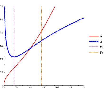
Figure 2. The curves represent the dispersion relation $\lambda(r)=\sqrt{r^{3}+r}$ and the group velocity $\lambda^{\prime}$, for $g=1=\sigma$. The frequency $\gamma_{1}$ corresponds to the space-time resonant sphere. Notice that while the slower decay at $\gamma_{0}$ is due to some degeneracy in the linear problem, $\gamma_{1}$ is unremarkable from the point of view of the linear dispersion.

Step 1. We would like to estimate now the increment of $\mathcal{E}_{N}(t)$. We use (3.36) and consider only the main case, when $|\xi|,|\eta|\approx 2^{k}\gg 1$, and $|\xi-\eta|$ is close to the slowly decaying frequency $\gamma_{0}$. So we need to bound space-time integrals of the form

$$I:=\int_{0}^{t}\int_{\mathbb{R}^{2}\times\mathbb{R}^{2}}m(\xi,\eta)\widehat{P_{k}W}(\eta,s)\widehat{P_{k}\overline{W}}(-\xi,s)\widehat{U}(\xi-\eta,s)\chi_{\gamma_{0}}(\xi-\eta)\,d\xi d\eta ds,$$

where $\chi_{\gamma_{0}}$ is a smooth cutoff function supported in the set $\{\xi:||\xi|-\gamma_{0}|\ll 1\}$, and we replaced $\Re u$ by $U$ (replacing $\Re U$ by $\overline{U}$ leads to a similar calculation). As before, define the linear profiles

$$u(t):=e^{it\Lambda}U(t),\qquad w(t):=e^{it\Lambda}W(t).$$ (3.39)

Then decompose the integral in dyadic pieces over the size of the modulation (3.41) and over the size of the time variable. In terms of the profiles $u,w$, we need to consider the space-time integrals

$$\begin{split}I_{k,m,p}:=\int_{\mathbb{R}}q_{m}(s)\int_{\mathbb{R}^{2}\times\mathbb{R}^{2}}e^{is\Phi(\xi,\eta)}&m(\xi,\eta)\widehat{P_{k}w}(\eta,s)\widehat{P_{k}\overline{w}}(-\xi,s)\\ &\times\widehat{u}(\xi-\eta,s)\chi_{\gamma_{0}}(\xi-\eta)\varphi_{p}(\Phi(\xi,\eta))\,d\xi d\eta ds,\end{split}$$ (3.40)

where

$$\Phi(\xi,\eta):=\Lambda(\xi)-\Lambda(\eta)-\Lambda(\xi-\eta)$$ (3.41)

is the associated modulation (or phase), $q_{m}$ is smooth and supported in the set $s\approx 2^{m}$ and $\varphi_{p}$ is supported in the set $\{x:|x|\approx 2^{p}\}$.

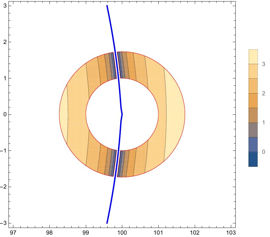
Figure 3. The first picture illustrates the resonant set $\{\eta:0=\Phi(\xi,\eta)=\Lambda(\xi)-\Lambda(\eta)-\Lambda(\xi-\eta)\}$ for a fixed large frequency $\xi$ (in the picture $\xi=(100,0)$). The second picture illustrates the intersection of a neighborhood of this resonant set with the set where $|\xi-\eta|$ is close to $\gamma_{0}$. Note in particular that near the resonant set $\xi-\eta$ is almost perpendicular to $\xi$ (see (3.38), (3.46)).

Step 2. To estimate the integrals $I_{k,m,p}$ we consider several cases depending on the relative size of $k,m,p$. Assume that $k,m$ are large, i.e. $2^{k}\gg 1,2^{m}\gg 1$, which is the harder case. To deal with the case of small modulation, when one cannot integrate by parts in time, we need an $L^{2}$ bound on the Fourier integral operator

$$T_{k,m,p}(f)(\xi):=\int_{{\mathbb{R}}^{2}}e^{is\Phi(\xi,\eta)}\varphi_{k}(\xi)\varphi_{\leq p}(\Phi(\xi,\eta))\chi_{\gamma_{0}}(\xi-\eta)f(\eta)\,d\eta,$$

where $s\approx 2^{m}$ is fixed. The critical bound proved in [60] (“the main $L^{2}$ lemma”) is

$$\|T_{k,m,p}(f)\|_{L^{2}}\lesssim_{\varepsilon}2^{{\varepsilon}m}(2^{(3/2)(p-k/2)}+2^{p-k/2-m/3})\|f\|_{L^{2}},\qquad{\varepsilon}>0,$$ (3.42)

provided that $p-k/2\in[-0.99m,-0.01m]$. The main gain here is the factor $3/2$ in $2^{(3/2)(p-k/2)}$ in the right-hand side (Schur’s test would only give a factor of $1$).

The proof of (3.42) uses a $TT^{\ast}$ argument, which is a standard tool to prove $L^{2}$ bounds for Fourier integral operators. This argument depends on a key nondegeneracy property of the function $\Phi$, more precisely on what we call the restricted nondegeneracy condition

$$\Upsilon(\xi,\eta)=\nabla_{\xi,\eta}^{2}\Phi(\xi,\eta)[\nabla_{\xi}^{\perp}\Phi(\xi,\eta),\nabla^{\perp}_{\eta}\Phi(\xi,\eta)]\neq 0\qquad\text{ if }\qquad\Phi(\xi,\eta)=0.$$ (3.43)

This condition, which appears to be new, can be verified explicitly in our case, when $||\xi-\eta|-\gamma_{0}|\ll 1$. The function $\Upsilon$ does in fact vanish at two points on the resonant set $\{\eta:\Phi(\xi,\eta)=0\}$ (where $||\xi-\eta|-\gamma_{0}|\approx 2^{-k}$), but our argument can tolerate vanishing up to order $1$.

The nondegeneracy condition (3.43) can be interpreted geometrically: the nondegeneracy of the mixed Hessian of $\Phi$ is a standard condition that leads to optimal $L^{2}$ bounds on Fourier integral operators. In our case, however, we have the additional cutoff function $\varphi_{\leq p}(\Phi(\xi,\eta))$, so we can only integrate by parts in the directions tangent to the level sets of $\Phi$. This explains the additional restriction to these directions in the definition of $\Upsilon$ in (3.43).

Given the bound (3.42), one can control the contribution of small modulations, i.e.

$$p-k/2\leq-2m/3-\epsilon m.$$ (3.44)

Step 3. In the high modulation case we integrate by parts in time in the formula (3.40). The main contribution is when the time derivative hits the high frequency terms, and the resulting integral is

$$\begin{split}I^{\prime}_{k,m,p}:=\int_{\mathbb{R}}q_{m}(s)\int_{\mathbb{R}^{2}\times\mathbb{R}^{2}}e^{is\Phi(\xi,\eta)}&m(\xi,\eta)\frac{d}{ds}\big{[}\widehat{P_{k}w}(\eta,s)\widehat{P_{k}\overline{w}}(-\xi,s)\big{]}\\ &\times\widehat{u}(\xi-\eta,s)\chi_{\gamma_{0}}(\xi-\eta)\frac{\varphi_{p}(\Phi(\xi,\eta))}{\Phi(\xi,\eta)}\,d\xi d\eta ds.\end{split}$$ (3.45)

Notice that $\partial_{t}w$ is a quadratic expression, as in (3.12), so that we gain a unit of decay (which is $|t|^{-5/6+}$), but lose a derivative.

In the harder case when the modulation is small we can use the depletion factor $\mathfrak{d}$ in the multiplier $m$, see (3.38), and the following key algebraic correlation

$$\text{ if }\qquad|\Phi(\xi,\eta)|\lesssim 1\qquad\text{ then }\qquad|m(\xi,\eta)|\lesssim 2^{-k}.$$ (3.46)

See Fig. 3. As a result, we gain one derivative in the integral $I^{\prime}_{k,m,p}$, which compensates for the derivative loss. On the other hand, when the modulation is not small, $2^{p}\geq 1$, then the denominator $\Phi(\xi,\eta)$ becomes a favorable factor, and one can reiterate the symmetrization procedure implicit in the energy estimates. This avoids the loss of one derivative and gives sufficient decay to estimate $|I^{\prime}_{k,m,p}|$, and close the energy estimate.

3.4.2. Dispersive analysis

The first main issue is to define an effective $Z$ norm that can be used in the bootstrap argument. As in (3.13), we use the Duhamel formula, written in terms of the profile $u=u_{+}=e^{it\Lambda}U$, $u_{-}=\overline{u}$,

$$\widehat{u}(\xi,t)=\widehat{u}(\xi,0)+\sum_{+,-}\int_{0}^{t}\int_{\mathbb{R}^{2}}e^{is[\Lambda(\xi)\mp\Lambda(\xi-\eta)\mp\Lambda(\eta)]}m_{\pm\pm}(\xi,\eta)\widehat{u_{\pm}}(\xi-\eta,s)\widehat{u_{\pm}}(\eta,s)\,d\eta ds,$$ (3.47)

where the sum is taken over choices of the signs $+,-$, and $m_{\pm\pm}$ are suitable smooth multipliers.

The idea is to estimate the function $\widehat{u}$ using the Duhamel formula (3.13), by integrating by parts either in $s$ or in $\eta$. As in (3.14)–(3.15), the main contribution is expected to come from the set of quadratic space-time resonances

$$\mathcal{SR}:=\{(\xi,\eta):\,\Phi(\xi,\eta)=0,\,(\nabla_{\eta}\Phi)(\xi,\eta)=0,\,m(\xi,\eta)\neq 0\},$$ (3.48)

where $m=m_{\pm\pm}$ and $\Phi(\xi,\eta)=\Lambda(\xi)\mp\Lambda(\xi-\eta)\mp\Lambda(\eta)$. In the gravity-capillary problem, space-time resonances are present only for the phase $\Phi(\xi,\eta)=\Lambda(\xi)-\Lambda(\xi-\eta)-\Lambda(\eta)$ and the space-time resonant set is

$$\{(\xi,\eta)\in\mathbb{R}^{2}\times\mathbb{R}^{2}:|\xi|=\gamma_{1}=\sqrt{2},\,\eta=\xi/2\}.$$ (3.49)

Moreover, the space-time resonant points are nondegenerate (according to the terminology of [85]), in the sense that the Hessian of the matrix $\nabla_{\eta\eta}^{2}\Phi(\xi,\eta)$ is non-singular at these points.

To gain intuition, consider the first iteration of the formula (3.13), i.e. assume that the functions $u_{\pm}$ in the right-hand side are Schwartz function supported at frequency $\approx 1$, independent of $s$. Assume that $s\approx 2^{m}$. Integration by parts in $\eta$ and $s$ shows that the main contribution comes from a small neighborhood of the stationary points where $|\nabla_{\eta}\Phi(\xi,\eta)|\leq 2^{-m/2+\delta m}$ and $|\Phi(\xi,\eta)|\leq 2^{-m+\delta m}$, up to negligible errors. Thus, the main contribution comes from space-time resonant points as in (3.14). A simple calculation shows that the main contribution to the second iteration is of the type

$$\widehat{u_{(2)}}(\xi)\approx c(\xi)\varphi_{\leq-m}(|\xi|-\gamma_{1}),$$

up to smaller contributions, where we have also ignored factors of $2^{\delta m}$, and $c$ is smooth.

We are now ready to describe more precisely the crucial choice of the $Z$ space. The idea is to decompose the profile as a superposition of atoms, localized in both space and frequency,

$$f={\sum}_{j,k}Q_{jk}f,\qquad Q_{jk}f=\varphi_{j}(x)\cdot P_{k}f(x).$$

The $Z$ norm is then defined by measuring suitably every atom.

In our case, the $Z$ space should include all Schwartz functions. It also has to include functions like $\widehat{u}(\xi)=\varphi_{\leq-m}(|\xi|-\gamma_{1})$, due to the considerations above, for any $m$ large. It should measure localization in both space and frequency, and be strong enough, at least, to recover the $t^{-5/6+}$ pointwise decay. We define

$$\|f\|_{Z_{1}}=\sup_{j,k}2^{j}\cdot\Big{\|}\big{|}|\xi|-\gamma_{1}\big{|}^{1/2}\widehat{Q_{jk}f}(\xi)\Big{\|}_{L^{2}_{\xi}},$$ (3.50)

up to small (but important) $\delta$-corrections. Then we define the $Z$ norm by applying a suitable number of vector-fields $D$ and $\Omega$.

We emphasize that the dispersive analysis in the $Z$ norm in the gravity-capillary problem is a lot more subtle than in the earlier papers on water waves. To illustrate how this analysis works in our problem, we consider the contribution of the integral over $s\approx 2^{m}\gg 1$ in (3.13), and assume that the frequencies are $\approx 1$.

Step 1. Start with the contribution of small modulations,

$$\widehat{u^{\prime}}(\xi):=\int_{\mathbb{R}}q_{m}(s)\int_{\mathbb{R}^{2}}\varphi_{\leq l}(\Phi(\xi,\eta))e^{is\Phi(\xi,\eta)}m_{++}(\xi,\eta)\widehat{u}(\xi-\eta,s)\widehat{u}(\eta,s)\,d\eta ds,$$ (3.51)

where $l=-m+\delta m$ ($\delta$ is a small constant) and $q_{m}(s)$ restricts the time integral to $s\approx 2^{m}$, and, for simplicity, we consider only the phase $\Phi(\xi,\eta)=\Lambda(\xi)-\Lambda(\xi-\eta)-\Lambda(\eta)$. In this case the considerations above, leading to the definition of the $Z$ norm, are still relevant: one can integrate by parts in $\eta$, identify the main contributions as coming from small $2^{-m/2+\delta m}$ neighborhoods of the stationary points, and estimate these contributions in the $Z$ norm.

Step 2. Consider now the contributions of the modulations of size $2^{l}$, $l\geq-m+\delta m$. We start from a formula similar to (3.51) and integrate by parts in $s$. The main case is when $d/ds$ hits one of the profiles $u$. Using again the equation (see (3.13)), we have to estimate cubic expressions of the form

$$\begin{split}\widehat{h_{m,l}}(\xi):=\int_{\mathbb{R}}q_{m}(s)&\int_{\mathbb{R}^{2}\times\mathbb{R}^{2}}\frac{\varphi_{l}(\Phi(\xi,\eta))}{\Phi(\xi,\eta)}e^{is\Phi(\xi,\eta)}m_{++}(\xi,\eta)\widehat{u}(\xi-\eta,s)\\ &\times e^{is\Phi^{\prime}(\eta,\sigma)}n(\eta,\sigma)\widehat{\overline{u}}(\eta-\sigma,s)\widehat{u}(\sigma,s)\,d\eta d\sigma ds,\end{split}$$ (3.52)

where $\Phi^{\prime}(\eta,\sigma)=\Lambda(\eta)+\Lambda(\eta-\sigma)-\Lambda(\sigma)$. We combine $\Phi$ and $\Phi^{\prime}$ into the cubic phase

$$\widetilde{\Phi}(\xi,\eta,\sigma):=\Phi(\xi,\eta)+\Phi^{\prime}(\eta,\sigma)=\Lambda(\xi)-\Lambda(\xi-\eta)+\Lambda(\eta-\sigma)-\Lambda(\sigma).$$

The most difficult case in the dispersive analysis is when $l$ is small, say $l\leq-m/14$, and the denominator $\Phi(\xi,\eta)$ in (3.52) is dangerous. We first restrict to suitably small neighborhoods of the stationary points of $\widetilde{\Phi}$ in $\eta$ and $\sigma$, thus to the cubic space-time resonances. Eventually we need to rely on one more algebraic property of the form

$$\text{ if }\quad\nabla_{\eta,\sigma}\widetilde{\Phi}(\xi,\eta,\sigma)=0\quad\text{ and }\quad|\Phi(\xi,\eta)|+|\Phi^{\prime}(\eta,\sigma)|\ll 1\quad\text{ then }\quad\nabla_{\xi}\widetilde{\Phi}(\xi,\eta,\sigma)=0.$$ (3.53)

The point of (3.53) is that in the resonant region for the cubic integral we have $\nabla_{\xi}\widetilde{\Phi}(\xi,\eta,\sigma)=0$, so the resulting function is essentially supported when $|x|\ll 2^{m}$, using an approximate finite speed of propagation argument. This gain is reflected in the factor $2^{j}$ in (3.50).

In proving control of the $Z$ norm, there are, of course, many cases to consider. The type of arguments presented above are typical in the proof: we decompose our profiles in space and frequency, localize to small sets in the frequency space, keeping track in particular of the special frequencies of size $\gamma_{0},\gamma_{1},\gamma_{1}/2,2\gamma_{0}$, use integration by parts in $\xi$ to control the location of the output, and use multilinear Hölder-type estimates to bound $L^{2}$ norms. An important aspect of this analysis is that we can essentially assume that all profiles are almost radial and located at frequencies $\lesssim 1$, thanks to the strong complementary control on Sobolev and weighted norms in the bootstrap hypothesis (3.35).

Step 3. The identity (3.47) can also be used to justify the approximate formula

$$(\partial_{t}\widehat{u})(\xi,t)\approx(1/t){\sum}_{j}\,\,g_{j}(\xi)e^{it\Phi(\xi,\eta_{j}(\xi))}+\,\text{lower order terms},$$ (3.54)

as $t\to\infty$, where $\eta_{j}(\xi)$ denote the stationary points where $\nabla_{\eta}\Phi(\xi,\eta_{j}(\xi))=0$. This approximate formula is consistent with the asymptotic behavior of solutions, more precisely scattering in the $Z$ norm. Qualitatively, at space-time resonances one has $\Phi(\xi,\eta_{j}(\xi))=0$, which leads to logarithmic growth for $\widehat{u}(\xi,t)$, while away from these space-time resonances the oscillation of $e^{it\Phi(\xi,\eta_{j}(\xi))}$ leads to convergence.

3.5. Conclusions and additional references

To summarize, there is a small number of cases when one can construct global solutions of water waves systems, by perturbing around the trivial solutions. The mechanism that leads to global solutions in all these cases is based on establishing dispersion and decay.

Sometimes it is possible to prove results going beyond the local theory, but not reach full global regularity. For example, starting with data of size ${\varepsilon}$ in a standard Sobolev space, one can sometimes get $\approx{\varepsilon}^{-2}$ time of existence by proving a quartic energy inequality like (3.25) in cases when there are no significant quadratic resonances (see [75, 82]). See also the recent work of Berti–Delort [22], where a combination of paradifferential analysis and ideas from KAM and normal forms theory was used to prove a significant long-time ($\approx{\varepsilon}^{-N}$) existence result for periodic 2D gravity-capillary waves (1D interface), for almost all choices of $(g,\sigma)$. Note that these extended lifespan results do not rely on dispersion but mainly on the absence of resonances.

In this context, a natural question to ask is if there are global or long-time regularity results for solutions with nontrivial vorticity. We emphasize that all the global regularity results so far assume irrotationality.

4. Formation of singularities and other topics

In this section we briefly present a few additional questions concerning the evolution of water waves, and provide more references to other topics.

4.1. Singularity formation

A set of fundamental questions in pure and applied fluid dynamics concerns the study of singularities. While some major open problems, such as the loss of regularity and blow-up in the (rotational) Euler flow, remain widely open, some types of “geometric singularities” have been studied in the context of water waves.

In [26] the authors proved that a wave that is initially given as the graph of a function $h$ can overturn at a later time. More importantly, Castro–Cordóba–Gancedo–Fefferman–Gómez-Serrano [27] showed the existence of “splash” singularities. A “splash” (resp. a “splat”) occurs when the surface of the fluid self-intersects at a point (resp. on an arc) while retaining its smoothness. This changes the topology of the domain, and leads to a breakdown of the chord-arc condition, that is, the assumption (to some extent necessary for well-posedness)

$$\sup_{\alpha\neq\beta\in{\mathbb{R}}}\frac{\alpha-\beta}{|z(t,\alpha)-z(t,\beta)|}<\infty,$$

where $z(t,\cdot):{\mathbb{R}}\rightarrow{\mathbb{R}}^{2}$ a parametrization of the interface $S_{t}$. Notice that a “splash” singularity occurs while the parametrization of the interface and the velocity of the fluid retain their initial regularity. The $2$d result of [27] was extended to $3$ dimensions and to some other related models by Coutand–Shkoller [43].

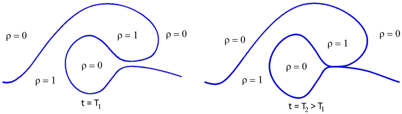
Figure 4. Formation of a “splash” singularity in 2D (taken from [27]).

In [66] Fefferman–Ionescu–Lie showed that a “splash” singularity cannot happen in the case of an interface separating two fluids: the presence of a second fluid, with positive constant density, prevents the interface from self-intersecting. In other words, one fluid cannot squeeze the other one if the interface and the solution are to remain smooth. A similar result was also proven by Coutand–Shkoller in [44]. We refer the reader to subsection 4.2 below for some references about the well-posedness and instability for interfaces between two fluids.

As discussed above, a self-intersection of an interface through a fluid cannot happen for sufficiently regular solutions of the water waves equations. However, it is plausible that a self-intersection could happen with the surface losing regularity, for example, pinching out and creating a cusp, see Figure 5 below.

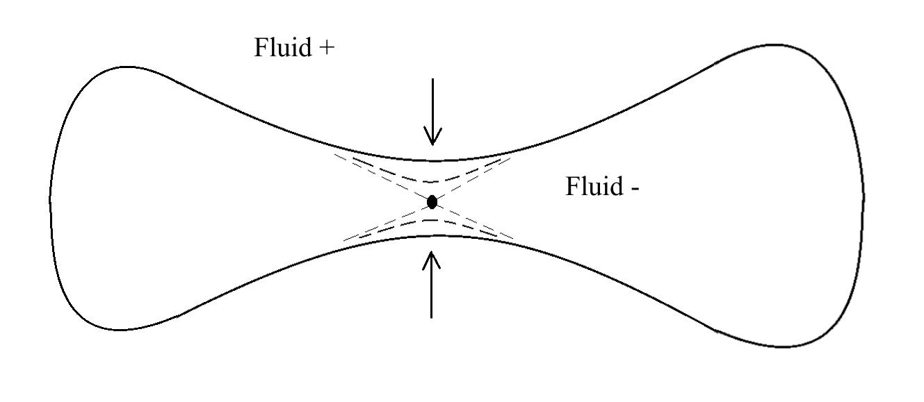
Figure 5. Possible scenario for a corner-like singularity: (1) a locally strong velocity field pushes two points to come close together, (2) the fluid in the middle does not have enough time to escape, (3) a self-intersection of the interface cannot happen with a smooth boundary, and the symmetries of the equation force the formation of a corner.

4.2. Fluid interfaces

In Section 2 we focused our attention on the evolution problem for one fluid in vaccum. When considering of the motion of waves on the surface of the ocean, one can think of the one-fluid model as a good first approximation for a water-air interface; rigorous results in this direction are provided by [112, 30, 100]. However, the motion of a free boundary between two immiscible fluids (or gases) is a more complex problem than (1.1).

The two-fluids model is a more unstable scenario than the one-fluid model and is subject to instabilities/ill-posedness in the absence of surface tension. Early works on this model and the study of its instability include [130, 65, 18, 83]. We also mention some classical numerical works by Hou–Lowengrub–Shelley [76, 77]. More recent contributions can be found in [11, 144, 121, 29, 30, 112, 100, 13] to cite a few. We refer the reader to the survey of Bardos–Lannes [17] for more on the instability of fluids interfaces.

We remark that there are no global regularity results for any two-fluids models.

4.3. Other questions and further references

The enormous complexity of the free boundary Euler flow and the water waves equations has motivated a large amount of research, beyond the local and global well-posedness discussed above. This includes the construction of particular classes of solutions, and extensive numerical activities. We provide here just a few additional references, including books and reviews, and other research papers on various topics of interest, and refer the reader to the cited works for more references on these topics.

• Steady, solitary, extreme waves. For the construction of steady water waves we refer to Groves’ survey [72] and the paper of Constantin–Strauss [39]; the excellent review of Strauss [128] contains an account on both the history and more modern achievements on this topic. See also the recent paper of Constantin–Strauss–Varvaruca [40] for the latest developments and more references.

  The existence theory of solitary waves was developed in Friedrichs–Hyers [67], Beale [19], Amick–Toland [15], Amick–Kirchgässner [16]; see also Rousset–Tzvetkov [114] for their transverse instability.

  The conjecture made by Stokes [126] that the crest of a steady wave of maximal amplitude forms a $120^{\circ}$ angle has been extensively investigated. Classical references on asymptotics are Longuet-Higgins–Fox [105, 106]; a proof of the conjecture was given by Amick–Fraenkel–Toland [14]; recent numerical works dealing with the behavior of near Stokes’ waves are in [63]. A counterpart of Stokes’ conjecture for large standing waves was proposed by Penney–Price in the ‘50s and its validity was investigated in [140]. Recent numerical computations of $3$d standing waves can be found in Rycroft–Wilkening [113]. See also [107, 36, 124, 135] for more properties of the profile of traveling gravity waves.

• Standing waves and Hamiltonian structure. An interesting aspect of the water waves equations concerns its Hamiltonian nature, which motivates numerous questions with a strong dynamical system flavor. An informative survey paper is Craig–Wayne [51]. Works in this direction, related to small divisors and Nash-Moser techniques, are those by Plotnikov–Toland [111], Iooss–Plotnikov–Toland [91], and Iooss–Plotnikov [90] on the existence of standing waves that are periodic in space and time. Quasi-periodic standing waves have been constructed by Berti–Montalto in [23] using KAM techniques for the first time in a quasilinear setting. See also the already mentioned work [22] where a key role is played by the reversible, rather than Hamiltonian, structure. Aspect of the theory of normal forms and connections to integrable Hamiltonian systems are discussed in many works, see for example [21, 151, 152, 52, 49, 46].

• Approximate and asymptotics models. Because of the physical relevance of the water waves system and the aim of better describing its complex dynamics, many simplified models have been derived and studied in special regimes. Two important examples include the approximation of waves in the form of wave packets by the nonlinear Schrödinger equation, and the approximation of long waves in shallow water by the KdV equation. We refer to [45, 116, 38, 10, 134], the book [101] and the surveys [115, 61] and references therein for more about reduced models and their mathematical justification.

• Books and reviews. An interesting historical account on the early developments of the theory can be found in Craik [53]. A classical introduction to the theory of water waves is Stoker [125]; an introduction to water waves and related models, such as KdV and NLS, can be found in Johnson [93], and a more thorough account in Sulem–Sulem [131]. The recent book of Lannes [101] contains all major results on the modern well-posedness theory and on approximate models, and the book of Constantin [37] discusses many applications to oceanography.

References

- [1] T. Alazard, N. Burq and C. Zuily. On the water waves equations with surface tension. Duke Math. J., 158 (2011), no. 3, 413-499.
- [2] T. Alazard, N. Burq and C. Zuily. On the Cauchy problem for gravity water waves. Invent. Math. 198 (2014), 71-163.
- [3] T. Alazard, N. Burq and C. Zuily. Strichartz estimates and the Cauchy problem for the gravity water waves equations. Preprint. arXiv:1404.4276.
- [4] T. Alazard, N. Burq and C. Zuily. Strichartz estimates for water waves. Ann. Sci. Éc. Norm. Supér., 44 (2011), no. 5, 855-903.
- [5] T. Alazard and J.M. Delort. Global solutions and asymptotic behavior for two dimensional gravity water waves. Ann. Sci. Éc. Norm. Supér. 48 (2015), 1149-1238.
- [6] T. Alazard and J.M. Delort. Sobolev estimates for two dimensional gravity water waves Astérisque 374 (2015) viii+241 pages.
- [7] T. Alazard and G. Métivier. Paralinearization of the Dirichlet to Neumann operator, and regularity of three-dimensional water waves. Comm. Partial Differential Equations, 34 (2009), no. 10-12, 1632-1704.
- [8] S. Alinhac. Paracomposition et opérateurs paradiffŕentiels. Comm. Partial Differential Equations, 11 (1986), no. 1, 87-121.
- [9] S. Alinhac. Existence d’ondes de raréfaction pour des systèmes quasi-linéaires hyperboliques multidimensionnels. Comm. Partial Differential Equations, 14 (1989), no. 2, 173-230.
- [10] B. Alvarez-Samaniego and D. Lannes. Large time existence for 3D water-waves and asymptotics. Invent. Math. 171 (2008), no. 3, 485-541.
- [11] D.M. Ambrose. Well-posedness of vortex sheets with surface tension. SIAM J. Math. Anal. 35 (2003), no. 1, 211-244.
- [12] D.M. Ambrose and N. Masmoudi. The zero surface tension limit of two-dimensional water waves. Comm. Pure Appl. Math. 58 (2005), no. 10, 1287-1315.
- [13] D.M. Ambrose and J. Wilkening. Computation of symmetric, time-periodic solutions of the vortex sheet with surface tension. PNAS, vol. 107 no. 8, 3361-3366.
- [14] C. J. Amick, L. E. Fraenkel and J. F. Toland. On the Stokes conjecture for the wave of extreme form. Acta Math. 148 (1982), 193-214.
- [15] C. J. Amick and J. F. Toland. On solitary water-waves of finite amplitude. Arch. Rational Mech. Anal. 76 (1981), no. 1, 9-95.
- [16] C. J. Amick and K. Kirchgässner. A theory of solitary water-waves in the presence of surface tension. Arch. Rational Mech. Anal. 105 (1989), no. 1, 1-49.
- [17] C. Bardos and D. Lannes. Mathematics for 2d interfaces. Singularities in mechanics: formation, propagation and microscopic description, 37-67, Panor. Synthèses, 38, Soc. Math. France, Paris, 2012.
- [18] C. Bardos, C. Sulem, P.-L. Sulem and U. Frisch. Finite time analyticity for the two- and three-dimensional Kelvin-Helmholtz instability. Comm. Math. Phys. 80 (1981), no. 4, 485-516.
- [19] J. T. Beale. The existence of solitary water waves. Comm. Pure Appl. Math. 30 (1977), 373-389.
- [20] J. T. Beale, T. Y. Hou and J. S. Lowengrub. Growth rates for the linearized motion of fluid interfaces away from equilibrium. Comm. Pure Appl. Math. 46 (1993), 1269-1301.
- [21] T. B. Benjamin and P. J. Olver. Hamiltonian structures, symmetries and conservation laws for water waves. J. Fluid Mech. 125 (1982), 137-187.
- [22] M. Berti and J. M. Delort. Almost global existence of solutions for capillarity-gravity water waves equations with periodic spatial boundary conditions. Preprint arXiv:1702.04674.
- [23] M. Berti and R. Montalto. Quasi-periodic standing wave solutions of gravity-capillary water waves. To appear in Mem. Amer. Math. Soc. arXiv:1602.02411.
- [24] K. Beyer and M. Günther. On the Cauchy problem for a capillary drop. I. Irrotational motion. Math. Methods Appl. Sci. 21 (1998), no. 12, 1149-1183.
- [25] J. M. Bony. Calcul symbolique et propagation des singularités pour les équations aux dérivées partielles non linéaires. Ann. Sci. École Norm. Sup. (4) 14 (1981), no. 2, 209-246.
- [26] A. Castro, D. Córdoba, C. Fefferman, F. Gancedo and M. López-Fernández. Rayleigh-Taylor breakdown for the Muskat problem with applications to water waves. Ann. of Math. 175 (2012), 909-948.
- [27] A. Castro, D. Córdoba, C. Fefferman, F. Gancedo and J. Gómez-Serrano. Finite time singularities for the free boundary incompressible Euler equations. Ann. of Math. 178 (2013), 1061-1134.
- [28] A-L Cauchy. Mémoire sur la th’eorie de la propagation des ondes à la surface d’un fluide pesant d’une profondeur indéfinie. Mém. Présentés Divers Savans Acad. R. Sci. Inst. France (Prix Acad. R. Sci., concours de 1815 et de 1816), I:3-312 (1827).
- [29] A. Cheng, D. Coutand and S. Shkoller. On the motion of Vortex Sheets with surface tension. Comm. Pure Appl. Math. 61 (2008), no. 12, 1715-1752.
- [30] A. Cheng, D. Coutand and S. Shkoller. On the limit as the density ratio tends to zero for two perfect incompressible 3-D fluids separated by a surface of discontinuity. Comm. Partial Differential Equations, 35 (2010), 817-845.
- [31] H. Christianson, V. Hur, and G. Staffilani. Strichartz estimates for the water-wave problem with surface tension. Comm. Partial Differential Equations 35 (2010), no. 12, 2195-2252.
- [32] D. Christodoulou and H. Lindblad. On the motion of the free surface of a liquid. Comm. Pure Appl. Math. 53 (2000), no. 12, 1536-1602.
- [33] D. Christodoulou and S. Klainerman. The global nonlinear stability of the Minkowski space. Princeton Mathematical Series 41. Princeton University Press, Princeton, NJ, 1993. x+514 pp.
- [34] J. Colliander, M. Keel, G. Staffilani, H. Takaoka and T. Tao. Sharp global well-posedness for KdV and modified KdV on and . J. Amer. Math. Soc. 16 (2003), no. 3, 705-749.
- [35] J. Colliander, M. Keel, G. Staffilani, H. Takaoka and T. Tao. Resonant decompositions and the I-method for the cubic nonlinear Schrödinger equation on . Discrete Contin. Dyn. Syst. 21 (2008), no. 3, 665-686.
- [36] A. Constantin. Comment on ”Steep sharp-crested gravity waves on deep water”. Phys. Rev. Lett. 93 (2004), 069402.
- [37] A. Constantin. Nonlinear Water Waves with applications to Wave-Current interactions and Tsunamis. CBMS-NSF Regional Conference Series in Applied Mathematics, 81. Society for Industrial and Applied Mathematics (SIAM), Philadelphia, PA, 2011. xii+321 pp.
- [38] A. Constantin and D. Lannes. The hydrodynamical relevance of the Camassa-Holm and Degasperis-Procesi equations. Arch. Ration. Mech. Anal. 192 (2009), no. 1, 165-186.
- [39] A. Constantin and W. Strauss. Exact steady periodic water waves with vorticity. Comm. Pure Appl. Math. 57 (2004), no. 4, 481-527.
- [40] A. Constantin, W. Strauss and E. Varvaruca. Global bifurcation of steady gravity water waves with critical layers, Acta Mathematica 217 (2016), 195-262.
- [41] D. Coutand. Finite time singularity formation for moving interface Euler equations Preprint arXiv:1701.01699.
- [42] D. Coutand and S. Shkoller. Well-posedness of the free-surface incompressible Euler equations with or without surface tension. J. Amer. Math. Soc. 20 (2007), no. 3, 829-930.
- [43] D. Coutand and S. Shkoller. On the finite-time splash and splat singularities for the 3-D free-surface Euler equations. Comm. Math. Phys. 325 (2014), 143-183.
- [44] D. Coutand and S. Shkoller. On the impossibility of finite-time splash singularities for vortex sheets. Arch. Ration. Mech. Anal. 221 (2016), no. 2, 987-1033.
- [45] W. Craig. An existence theory for water waves and the Boussinesq and Korteweg-de Vries scaling limits. Comm. Partial Differential Equations, 10 (1985), no. 8, 787-1003
- [46] W. Craig. Birkhoff normal forms for water waves. Mathematical problems in the theory of water waves (Luminy, 1995), 57-74. Contemp. Math., 200, Amer. Math. Soc., Providence, RI, 1996.
- [47] W. Craig. On the Hamiltonian for water waves. Preprint arXiv:1612.08971.
- [48] W. Craig, U. Schanz and C. Sulem. The modulational regime of three-dimensional water waves and the Davey-Stewartson system. Ann. Inst. H. Poincaré Anal. Non Linéaire, 14 (1997), no. 5, 615-667.
- [49] W. Craig and C. Sulem. Mapping properties of normal forms transformations for water waves. Boll. Unione Mat. Ital. 9 (2016), no. 2, 289-318.
- [50] W. Craig, C. Sulem and P.-L. Sulem. Nonlinear modulation of gravity waves: a rigorous approach. Nonlinearity 5 (1992), no. 2, 497-522.
- [51] W. Craig and C. E. Wayne. Mathematical aspects of surface waves on water. Russian Math. Surveys 62 (2007), no. 3, 453-473.
- [52] W. Craig and C. P. A. Worfolk. An integrable normal form for water waves in infinite depth. Phys. D 84 (1995), no. 3-4, 513-531.
- [53] A.D.D. Craik. The origins of water wave theory. Annual review of fluid mechanics. Vol. 36, 1-28. Annu. Rev. Fluid Mech., 36, Annual Reviews, Palo Alto, CA, 2004.
- [54] T. De Poyferré. A priori estimates for water waves with emerging bottom. arXiv:1612.04103. Preprint.
- [55] T. de Poyferré and Q.-H. Nguyen. Strichartz estimates and local existence for the gravity-capillary waves with non-Lipschitz initial velocity. J. Differential Equations 261 (2016), no. 1, 396-438.
- [56] B. Deconinck and K. Oliveras. The instability of periodic surface gravity waves. J. Fluid Mech. 675 (2011), 141-167.
- [57] J.M. Delort. Global existence and asymptotic behavior for the quasilinear Klein-Gordon equation with small data in dimension 1. Ann. Sci. École Norm. Sup. 34 (2001), no. 1, 1-61.
- [58] J.M. Delort. Long-time Sobolev stability for small solutions of quasi-linear Klein-Gordon equations on the circle. Trans. Amer. Math. Soc. 361 (2009), 4299-4365.
- [59] Y. Deng, A. D. Ionescu and B. Pausader. The Euler-Maxwell system for electrons: global solutions in 2D. Preprint (2015).
- [60] Y. Deng, A. D. Ionescu, B. Pausader, and F. Pusateri. Global solutions for the gravity-capillary water waves system. Preprint arXiv:1601.05685.
- [61] W.-P. Düll. On the mathematical description of water waves. Preprint arXiv:1612.06242.
- [62] A. I. Dyachenko, E. A. Kuznetsov, M. Spector and V. E. Zakharov. Analytical description of the free surface dynamics of an ideal fluid (canonical formalism and conformal mapping). Phys. Lett. A 221 (1996), 73-79.
- [63] S. A. Dyachenko, P. M. Lushnikov and A. O. Korotkevich. The complex singularity of a Stokes wave. JETP Lett. 98 (2013), 767-771.
- [64] G. Ebin. The equations of motion of a perfect fluid with free boundary are not well posed. Comm. Partial Differential Equations 12 (1987), no. 10, 1175-1201.
- [65] G. Ebin. Ill-posedness of the Raileigh-Taylor and Kelvin-Helmotz problems for for incompressible fluids. Comm. Partial Differential Equations, 13 (1988), no. 10, 1265-1295.
- [66] C. Fefferman, A. D. Ionescu and V. Lie. On the absence of “splash” singularities in the case of two-fluid interfaces. Duke Math. J. 165 (2016), no. 3, 417-462.
- [67] K. Friedrichs and D. Hyers. The existence of solitary waves. Comm Pure Appl. Math. 7 (1954), 517-550.
- [68] R. Gerber. Sur les solutions exactes des équations du mouvement avec surface libre d’un liquide pesant. J Math Pure Appl. 34 (1955), 185-299.
- [69] P. Germain and N. Masmoudi. Global existence for the Euler-Maxwell system. Ann. Sci. Éc. Norm. Supér. (4) 47 (2014), no. 3, 469-503.
- [70] P. Germain, N. Masmoudi and J. Shatah. Global solutions for the gravity surface water waves equation in dimension 3. Ann. of Math., 175 (2012), 691-754.
- [71] P. Germain, N. Masmoudi and J. Shatah. Global solutions for capillary waves equation in dimension 3. Comm. Pure Appl. Math. 68 (2015), no. 4, 625-687.
- [72] M. Groves. Steady water waves. J. Nonl. Math. Phys. 11 (2004), 435-460.
- [73] Y. Guo, A. D. Ionescu and B. Pausader. Global solutions of the Euler-Maxwell two-fluid system in 3D. To appear in Ann. of Math. arXiv:1303.1060.
- [74] S. Gustafson, K. Nakanishi and T. Tsai. Scattering for the Gross-Pitaevsky equation in 3 dimensions. Commun. Contemp. Math. 11 (2009), no. 4, 657-707.
- [75] B. Harrop-Griffiths, M. Ifrim and D. Tataru. Finite depth gravity water waves in holomorphic coordinates. Preprint arXiv:1607.02409.
- [76] T. Y. Hou, J. S. Lowengrub and M. Shelley. Removing the stiffness from interfacial flows with surface tension. J. Comput. Phys. 114 (1994), no. 2, 312-338.
- [77] T. Y. Hou, J. S. Lowengrub and M. Shelley. The long-time motion of vortex sheets with surface tension. J. Phys. Fluids 9 (1997), no. 7, 1933-1954.
- [78] J. Hunter, M. Ifrim, D. Tataru and T. Wong. Long time solutions for a Burgers-Hilbert equation via a modified energy method. Proc. Amer. Math. Soc. 143 (2015), 3407-3412.
- [79] J. Hunter, M. Ifrim and D. Tataru. Two dimensional water waves in holomorphic coordinates. Comm. Math. Phys. 346 (2016), 483-552.
- [80] M. Ifrim and D. Tataru. Two dimensional water waves in holomorphic coordinates II: global solutions. Bull. Soc. Math. France 144 (2016), 369-394.
- [81] M. Ifrim and D. Tataru. The lifespan of small data solutions in two dimensional capillary water waves. Preprint arXiv:1406.5471.
- [82] M. Ifrim and D. Tataru. Two dimensional gravity water waves with constant vorticity: I. Cubic lifespan. Preprint arXiv:1510.07732.
- [83] T. Iguchi, N. Tanaka and A. Tani. On the two-phase free boundary problem for two-dimensional water waves. Math. Ann. 309 (1997), no. 2, 199-223.
- [84] A. D. Ionescu and B. Pausader. The Euler-Poisson system in 2D: global stability of the constant equilibrium solution. Int. Math. Res. Not. (2013), no. 4, 761-826.
- [85] A. D. Ionescu and B. Pausader. Global solutions of quasilinear systems of Klein-Gordon equations in 3D. J. Eur. Math. Soc. 16 (2014), no. 11, 2355-2431.
- [86] A. D. Ionescu and F. Pusateri. Nonlinear fractional Schrödinger equations in one dimension. J. Funct. Anal. 266 (2014), 139-176.
- [87] A. D. Ionescu and F. Pusateri. Global solutions for the gravity water waves system in 2D. Invent. Math. 199 (2015), no. 3, 653-804.
- [88] A. D. Ionescu and F. Pusateri. Global analysis of a model for capillary water waves in 2D. Comm. Pure Appl. Math. 69 (2016), no. 11, 2015-2071.
- [89] A. D. Ionescu and F. Pusateri. Global regularity for 2d water waves with surface tension. To appear in Mem. Amer. Math. Soc. arXiv:1408.4428.
- [90] G. Iooss and P. I. Plotnikov. Small divisor problem in the theory of three-dimensional water gravity waves. Mem. Amer. Math. Soc. 200 (2009), no. 940, viii+128 pp.
- [91] G. Iooss, P. I. Plotnikov and J. F. Toland. Standing waves on an infinitely deep perfect fluid under gravity. Arch. Ration. Mech. Anal. 177 (2005), no. 3, 367-478.
- [92] F. John. Blow-up for quasilinear wave equations in three space dimensions. Comm. on Pure Appl. Math. 34 (1981), no. 1, 29-51.
- [93] R. S. Johnson. A modern introduction to the mathematical theory of water waves. Cambridge Texts in Applied Mathematics. Cambridge University Press, Cambridge, 1997. xiv+445 pp.
- [94] T. Kano and T. Nishida. Sur les ondes de surface de l’eau avec une justification mathématique des équations des ondes en eau peu profonde. J. Math. Kyoto Univ. 19 (1979), no. 2, 335-370.
- [95] R. H. Kinsey and S. Wu. A Priori Estimates for Two-Dimensional Water Waves with Angled Crests Preprint arXiv:1406.7573.
- [96] S. Klainerman. Uniform decay estimates and the Lorentz invariance of the classical wave equation. Comm. Pure Appl. Math. 38 (1985), no. 3, 321-332.
- [97] S. Klainerman. The null condition and global existence for systems of wave equations. Nonlinear systems of partial differential equations in applied mathematics, Part 1 (Santa Fe, N.M., 1984), 293-326. Lectures in Appl. Math., 23, Amer. Math. Soc., Providence, RI, 1986.
- [98] I. Kukavica, A. Tuffaha and V. Vicol. On the Local Existence and Uniqueness for the 3D Euler Equation with a Free Interface. Appl. Math. Optim. (2016), 1-29.
- [99] D. Lannes. Well-posedness of the water waves equations. J. Amer. Math. Soc. 18 (2005), no. 3, 605-654.
- [100] D. Lannes. A stability criterion for two-fluid interfaces and applications. Arch. Ration. Mech. Anal. 208 (2013), no. 2, 481-567.
- [101] D. Lannes. The water waves problem. Mathematical analysis and asymptotics. Mathematical Surveys and Monographs, Vol. 188. American Mathematical Society, Providence, RI, 2013. xx+321 pp.
- [102] D. Lannes. On the dynamics of floating structures. Preprint arXiv:1609.06136.
- [103] T. Levi-Civita. Détermination rigoureuse des ondes permanentes d’ampleur finie. Math. Ann. 93 (1925), no. 1, 264-314.
- [104] H. Lindblad. Well-posedness for the motion of an incompressible liquid with free surface boundary. Ann. of Math. 162 (2005), no. 1, 109-194.
- [105] M. S. Longuet-Higgins and M. J. H. Fox. Theory of the almost-highest wave: The inner solution. J . Fluid Mech. (1977), vol. 80, 721-741.
- [106] M. S. Longuet-Higgins and M. J. H. Fox. Theory of the almost-highest wave. Part 2. Matching and analytic extension J . Fluid Mech. 85 (1978), 769-786.
- [107] V. Lukomsky, I. Gandzha, and D. Lukomsky. Steep sharp-crested gravity waves on deep water. Phys. Rev. Lett. 89 (2002), 164502.
- [108] G. Métivier. Para-differential calculus and applications to the Cauchy problem for nonlinear systems. Centro di Ricerca Matematica Ennio De Giorgi (CRM) Series, 5. Edizioni della Normale, Pisa, 2008. xii+140 pp.
- [109] M. Ming and Z. Zhang. Well-posedness of the water-wave problem with surface tension. J. Math. Pures Appl. (9) 92 (2009), no. 5, 429-455.
- [110] V. I. Nalimov. The Cauchy-Poisson problem. Dinamika Splosn. Sredy Vyp. 18 Dinamika Zidkost. so Svobod. Granicami (1974), 10-210, 254.
- [111] P. I. Plotnikov and J. F. Toland. Nash-Moser theory for standing waves. Arch. Ration. Mech. Anal. 159 (2001), no. 1, 1-83.
- [112] F. Pusateri. On the limit as the surface tension and density ratio tend to zero for the two phase Euler equation. J. Hyperbolic Differ. Equ. 8 (2011), no. 2, 347-373.
- [113] C. H. Rycroft and J. Wilkening. Computation of three-dimensional standing water waves. J. Comput. Phys. 255 (2013), 612-638.
- [114] F. Rousset and N. Tzvetkov. Transverse instability of the line solitary water-waves. Invent. Math. 184 (2011), no. 2, 257-388.
- [115] G. Schneider and C. E. Wayne. On the validity of 2D-surface water wave models. GAMM Mitt. Ges. Angew. Math. Mech. 25 (2002), no. 1-2, 127-151.
- [116] G. Schneider and C. E. Wayne. The rigorous approximation of long-wavelength capillary-gravity waves. Arch. Ration. Mech. Anal. 162 (2002), no. 3, 247-285.
- [117] B. Schweizer. On the three-dimensional Euler equations with a free boundary subject to surface tension. Ann. Inst. H. Poincaré Anal. Non Linéaire 22 (2005), 753-781.
- [118] J. Shatah. Normal forms and quadratic nonlinear Klein-Gordon equations. Comm. Pure Appl. Math. 38 (1985), no. 5, 685-696.
- [119] J. Shatah and C. Zeng. Geometry and a priori estimates for free boundary problems of the Euler equation. Comm. Pure Appl. Math. 61 (2008), no. 5, 698-744.
- [120] J. Shatah and C. Zeng. A priori estimates for fluid interface problems. Comm. Pure Appl. Math. 61 (2008), no. 6, 848-876.
- [121] J. Shatah and C. Zeng. Local well-posedness for the fluid interface problem. Arch. Ration. Mech. Anal. 199 (2011), no. 2, 653-705.
- [122] M. Shinbrot. The initial value problem for surface waves under gravity. I. The simplest case. Indiana Univ. Math. J. 25 (1976), no. 3, 281-300.
- [123] T. C. Sideris. Formation of singularities in three-dimensional compressible fluids. Comm. Math. Phys. 101 (1985), no. 4, 475-485.
- [124] E. R. Spielvogel. A variational principle for waves of infinite depth. Arch. Rational Mech. Anal. 39 (1970), 189-205.
- [125] J. J. Stoker. Water waves. The mathematical theory with applications. Wiley Classics Library. A Wiley-Interscience Publication. John Wiley & Sons, Inc., New York, 1992. xxvi+567 pp.
- [126] G. G. Stokes. On the theory of oscillatory waves. Trans. Cambridge Philos. Soc., 8 (1847), 441-455.
- [127] G. G. Stokes. Considerations relative to the greatest height of oscillatory irrotational waves which can be propagated without change of form (1880). Mathematical and Physical Papers, Volume 1, pages 225-228.
- [128] W. Strauss. Steady water waves. Bull. Amer. Math. Soc. (N.S.) 47 (2010), no. 4, 671-694.
- [129] D. J. Struik. Détermination rigoureuse des ondes irrotationelles périodiques dans un canal à profondeur finie. Math. Ann. 95 (1926), no. 1, 595-634.
- [130] C. Sulem and P.L. Sulem. The well-posedness of two-dimensional ideal flow. J. Méc. Théor. Appl. 1983, Special Issue, 217-242.
- [131] C. Sulem and P.L. Sulem. The nonlinear Schrödinger equation. Self-focussing and wave collapse. Applied Mathematical Sciences, 139. Springer-Verlag, New York, 1999.
- [132] G. I. Taylor. The instability of liquid surfaces when accelerated in a direction perpendicular to their planes I. Proc. Roy. Soc. London A 201 (1950) 192-196.
- [133] M. Taylor. Tools for PDE. Pseudodifferential operators, paradifferential operators, and layer potentials. Mathematical Surveys and Monographs, 81. American Mathematical Society, Providence, RI, 2000. x+257 pp.
- [134] N. Totz and S. Wu. A rigorous justification of the modulation approximation to the 2D full water wave problem. Comm. Math. Phys. 310 (2012), no. 3, 817-883.
- [135] E. Varvaruca. Some geometric and analytic properties of solutions of Bernoulli free-boundary problems. Interfaces Free Bound. 9 (2007), 367-381.
- [136] X. Wang. Global infinite energy solutions for the 2D gravity water waves system. Preprint arXiv: 1502.00687.
- [137] X. Wang. On 3D water waves system above a flat bottom. Preprint arXiv:1508.06223.
- [138] X. Wang. Global solution for the 3D gravity water waves system above a flat bottom. Preprint arXiv:1508.06227.
- [139] X. Wang. Global regularity for the 3D finite depth capillary water waves. Preprint arXiv:1611.05472.
- [140] J. Wilkening. Breakdown of Self-Similarity at the Crests of Large-Amplitude Standing Water Waves. Phys. Rev. Lett. (2011) 107, 184501.
- [141] J. Wilkening and V. Vasal. Comparison of five methods of computing the Dirichlet-Neumann operator for the water wave problem. Nonlinear wave equations: analytic and computational techniques 175-210, Contemp. Math., 635, Amer. Math. Soc., Providence, RI, 2015.
- [142] S. Wu. Well-posedness in Sobolev spaces of the full water wave problem in 2-D. Invent. Math. 130 (1997), 39-72.
- [143] S. Wu. Well-posedness in Sobolev spaces of the full water wave problem in 3-D. J. Amer. Math. Soc. 12 (1999), 445-495.
- [144] S. Wu. Mathematical analysis of vortex sheets. Comm. Pure Appl. Math. 59 (2006), no. 8, 1065-1206.
- [145] S. Wu. Almost global wellposedness of the 2-D full water wave problem. Invent. Math. 177 (2009), 45-135.
- [146] S. Wu. Global wellposedness of the 3-D full water wave problem. Invent. Math. 184 (2011), 125-220.
- [147] S. Wu. A blow-up criteria and the existence of 2d gravity water waves with angled crests. Preprint arXiv:1502.05342.
- [148] S. Wu. Wellposedness and singularities of the water wave equations. Lectures on the theory of water waves, 171-202, London Math. Soc. Lecture Note Ser., 426, Cambridge Univ. Press, Cambridge, 2016.
- [149] H. Yosihara. Gravity waves on the free surface of an incompressible perfect fluid of finite depth. Publ. Res. Inst. Math. Sci. 18 (1982), 49-96.
- [150] V. E. Zakharov. Stability of periodic waves of finite amplitude on the surface of a deep fluid. Zhurnal Prikladnoi Mekhaniki i Teckhnicheskoi Fiziki 9 (1968), no.2, 86-94. J. Appl. Mech. Tech. Phys., 9, 1990-1994.
- [151] V. E. Zakharov. Weakly nonlinear waves on the surface of an ideal finite depth fluid. Nonlinear waves and weak turbulence, 167-197, Amer. Math. Soc. Transl. Ser. 2, 182, Amer. Math. Soc., Providence, RI, 1998.
- [152] V. E. Zakharov and A. I. Dyachenko. Is free-surface hydrodynamics an integrable system? Phys. Lett. A 190 (1994), no. 2, 144-148.
- [153] V. E. Zakharov and A. I. Dyachenko. High-Jacobian approximation in the free surface dynamics of an ideal fluid. Nonlinear phenomena in ocean dynamics (Los Alamos, NM, 1995). Phys. D 98 (1996), no. 2-4, 652-664.
- [154] P. Zhang and Z. Zhang. On the free boundary problem of three-dimensional incompressible Euler equations. Comm. Pure Appl. Math. 61 (2008), no. 7, 877-940.