Toward an Empirical Theory of Pulsar Emission XII: Exploring the
Physical Conditions in Millisecond Pulsar Emission Regions

Abstract

The five-component profile of the 2.7-ms pulsar J0337+1715 appears to exhibit the best example to date of a core/double-cone emission-beam structure in a millisecond pulsar (MSP). Moreover, three other MSPs, the Binary Pulsar B1913+16, B1953+29 and J1022+1001, seem to exhibit core/single-cone profiles. These configurations are remarkable and important because it has not been clear whether MSPs and slow pulsars exhibit similar emission-beam configurations, given that they have considerably smaller magnetospheric sizes and magnetic field strengths. MSPs thus provide an extreme context for studying pulsar radio emission. Particle currents along the magnetic polar flux tube connect processes just above the polar cap through the radio-emission region to the light-cylinder and the external environment. In slow pulsars radio-emission heights are typically about 500 km around where the magnetic field is nearly dipolar, and estimates of the physical conditions there point to radiation below the plasma frequency and emission from charged solitons by the curvature process. We are able to estimate emission heights for the four MSPs and carry out a similar estimation of physical conditions in their much lower emission regions. We find strong evidence that MSPs also radiate by curvature emission from charged solitons.

1. Introduction

Millisecond pulsar (MSP) emission processes have remained enigmatic despite the very prominence of MSPs as indispensable tools of contemporary physics and astrophysics. MSP magnetospheres are much more compact ($\sim$100 to 3000 km), and their magnetic field strengths are typically 10${}^{3}$-10${}^{4}$ times weaker and probably more complex than those of normal pulsars, due to the period of accretion that is believed to recycle old pulsars into MSPs.

Normal pulsars are found to exhibit many regularities of profile form and polarization that, together, suggest an overall beam geometry comprised by two distinct emission cones and a central core beam. It would seem that these regularities occur in major part because the magnetic field, at the roughly 500-km height where radio emission occurs, is usually highly dipolar (Rankin, Melichidze & Mitra 2017).

The vast majority of MSPs show no such regularity. Their polarized profile forms are often broad and complex and seem almost a drunken parody of the order that is exhibited by many slower pulsars [e.g., Dai et al  (2015) and the references therein]. The reasons for this disorder are not yet fully clear, but the smaller magnetospheres of MSPs may well entail emission heights where the magnetic fields are dominated by quadrupoles and higher terms. Also, aberration/retardation (hereafter A/R) becomes ever more important for faster pulsars. In this context, it is arresting to encounter a few MSPs that appear to exhibit the regular profile forms and perhaps polarization of normal pulsars. If so, even a few such MSPs provide an opportunity to work out their quantitative emission geometry and assess whether their radiative processes are similar to those of normal pulsars.

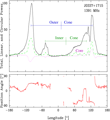
Figure 1.— Total 1.4-GHz Arecibo PUPPI polarized profile of pulsar J0337+1715 showing its apparent core component as well as its pairs of inner and outer conal components. The core component seems to be conflated with the trailing conal components at about 90° longitude. The positions and centers of the two conal component pairs are indicated. They are far from symmetrically spaced as in slower pulsars, apparently because of aberration/retardation. However, note that the outer cone center precedes the inner one as well as the core. The upper panel gives the total intensity (Stokes $I$; solid curve), the total linear ($L$ [=$\sqrt{Q^{2}+U^{2}}$]; dashed green), and the circular polarization (Stokes $V$; dotted magenta). The PPA [=$(1/2)\tan^{-1}(U/Q)$] values (lower panel) have been Faraday-derotated to infinite frequency. Errors in the PPAs were computed relative to the off-pulse noise phasor—that is, $\sigma_{PPA}\sim tan^{-1}(\sigma_{\mathrm{off-pulse}}/L)$ and are plotted when $<30\arcdeg$ and indicated by occasional 3-$\sigma$ error bars.

The profile of millisecond pulsar J0337+1715 surprisingly has what appears to be a five-component core/double-cone configuration. Such a five-component structure is potentially important because it has not been clear whether millisecond pulsars ever exhibit emission-beam configurations similar to those of slower pulsars. J0337+1715 is now well known as the unique example so far of a millisecond pulsar in a system of three stars (Ransom et al  2014). The pulsar is relatively bright and can be observed over a large frequency band, so that both its pulse timing and polarized profile characteristics can be investigated in detail.

In addition, we find three other probable examples of MSPs with core-cone profiles: the original binary pulsar, B1913+16; the second MSP discovered, B1953+29; and pulsar J1022+1001. We will also discuss the profile geometries of these three MSPs and consider their interpretations below.

The slow pulsars with four-component profiles show outer and inner pairs of conal components, centered closely on the (unseen) longitude of the magnetic axis, all with particular dimensions relative to the angular size of the pulsar’s magnetic (dipolar) polar cap. The classes of pulsar profiles and their quantitative beaming geometries are discussed in Rankin (1983, ET I) and ET VI, and other population analyses have come to similar conclusions (e.g., Gil et al  1993; Mitra & Deshpande 1999; Mitra & Rankin 2011). Core beams have intrinsic half-power angular diameters about equal to a pulsar’s (dipolar) polar cap ($2.45\arcdeg P^{-1/2}$, where $P$ is the pulsar rotation period), suggesting generation at altitudes just above the polar cap. Conal beam radii in slow pulsars also scale as $P^{-1/2}$ and reflect emission from heights of several hundred km. Core emission heights are not usually known apart from the low altitude implication of their widths—so it is plausible to assume that core radiation arises from heights well below that of the conal emission.

Classification of profiles and quantitative geometrical modeling provides an essential foundation for understanding pulsars physically. MSPs, heretofore, have seemed inexplicable in these terms. The core/double-cone model works well for most pulsars with periods longer than about 100 ms, whereas faster pulsars mostly either present inscrutable single profiles or complex ones where no cones or core can be identified. It is then important to learn how and why it is that the core/double-cone beam model often breaks down for the faster pulsars.

Aberration/retardation (hereafter A/R) becomes more important for faster pulsars and MSPs simply because their periods are shorter compared to A/R temporal shifts. The role of A/R in pulsar emission profiles was first described by Blaskiewicz et al  (1991, hereafter BCW), but only later was this understanding developed into a reliable technique for determining pulsar emission heights (e.g., Dyks et al  2004; Dyks 2008; Mitra & Rankin 2011; Kumar & Gangadhara 2012). A/R has the effect of shifting the profile earlier and the polarization-angle (hereafter PPA) traverse later by equal amounts

$$\Delta t=\pm 2h_{em}/c$$ (1)

where $h_{em}$ is the emission height (above the center of the star), such that the magnetic axis longitude remains centered in between. In that the PPA inflection is often difficult to determine, A/R heights have also been estimated by using the core position as a marker for the magnetic axis longitude as first suggested by Malov & Suleimanova (1998) and Gangadhara & Gupta (2001) and now widely used. The A/R method has thus usually been used to measure conal emission heights, but core heights have also been estimated for B0329+54 (Mitra et al  2007) and recently for B1933+16 and several other pulsars (Mitra et al  2016) giving heights around or a little lower than the conal ones. Crucially, A/R measurements indicate emission heights of some 300-500 km in the slow pulsar population. So it is important to see how MSPs compare, given that many have magnetospheres smaller than 500 km.

In what follows we discuss the observations in §2, the J0337+1715 core component and its width in §3.1, and the conal component configuration in §3.2. §3.3 treats its quantitative geometry, §3.4 computes aberration/retardation emission heights, and §4 considers three other millisecond pulsars with cone/single-cone profiles. Finally, §5 summarizes the results, §LABEL:phys interprets them physically, and §LABEL:con outlines the overall conclusions.

Table 1Properties of the Arecibo and GBT observations.

Band	Backend	MJD	Resolution	Length
(GHz)			(°/sample)	(s)
J0337+1715 ($P$=2.73 msec; $DM$=21.32 pc/cm${}^{3}$)
1.1-1.7	PUPPI	56736	0.70	$\sim$3400
1.1-1.8	GUPPI	56412	0.70	40968
0.42-0.44	PUPPI	56584	1.41	$\sim$3400
1.9-2.5*	PUPPI	56781	1.41	3600
1.9-2.5	PUPPI	57902	1.41	3600
2.5-3.1*	PUPPI	56768	1.41	3936
2.5-3.1	PUPPI	57902	1.41	3000
1.1-1.7	Mocks	56760	4.74	1000
B1913+16 ($P$=59.0 msec; $DM$=168.77 pc/cm${}^{3}$)
1.1-1.9	GUPPI	55753	0.35	1900
1.1-1.7	Mocks	56199	0.58	1200
B1953+29 ($P$=6.13 msec; $DM$=104.501 pc/cm${}^{3}$)
1.1-1.6	Mocks	56564	2.24	2400
1.1-1.6	Mocks	56585	2.24	2400
1.1-1.9	PUPPI	57129	0.35	3608
J1022+1001 ($P$=16.4 msec; $DM$=10.2521 pc/cm${}^{3}$)
1.1-1.7	Mocks	56315/23	0.53	600
1.1-1.7	Mocks	56577	0.46	1800
0.30-0.35	Mocks	56418/31	2.55	600
0.30-0.35	Mocks	56577	2.55	1800

Notes: These earlier PUPPI 2.0- and 2.8-GHZ observations could not be calibrated polarimetrically because of faulty cal signals; therefore, we use only Stokes $I$ in Figure LABEL:figA1.

2. Observations

2.1. Acquisition and calibration

J0337+1715 A large number of observations at different frequencies and observatories were carried out in the course of confirming J0337+1715 and understanding the complex orbital modulations of its pulse-arrival times. Some of these were polarimetric and some much more sensitive, and unsurprisingly the Arecibo observations were usually the highest quality. In compiling the observations for this analysis, we assessed which observations were deepest at both 1400 and 430 MHz. The PUPPI backend was used at both frequencies with a 30-MHz bandwidth at 430 and a 600-MHz bandwidth at 1400 MHz. We then explored the pulsar’s behavior at higher frequencies, and both 2.0 and 2.8-GHz observations are reported here. We also attempted a rise-to-set observation at 5 GHz with a 1-GHz bandwidth, but the pulsar was not detected. All the J0337+1715 observations were calibrated or re-calibrated using the PSRchive pac -x routine (Hotan, van Straten & Manchester 2004). The final bin size was chosen to reflect the joint time and frequency resolution, and is given in Table 1 along with some other characteristics of the observations.

The 1391-MHz profile in Fig. 1 is the deepest and best resolved of the four and deserves more detailed analysis. The 2.8, 2.0 and 0.43 GHz profiles can be seen in Fig. 2.

B1913+16, B1953+29 and J1022+1001. We also carried out Arecibo observations of these pulsars using the L-band Wide feed and the Mock spectrometers. The former were single-pulse polarimetric observations using as many Mocks as needed to optimize the resolution and use the total available bandwidth for maximal sensitivity, and the results are given in Table 1. These Mock observations were processed as described in Mitra et al  (2016) including derotation to infinite frequency.

2.2. Rotation-measure determinations

Our rotation-measure determinations will be published as a part of a larger paper in preparation together with a full description of our observations and techniques.

J0337+1715. A rotation measure ($RM$) of +30$\pm$3 rad-m${}^{2}$ was determined using a set of the best quality observations from both the Arecibo PUPPI and Green Bank Telescope (hereafter GBT) GUPPI machines. These were processed as above with PSRchive, and its rmfit routine was used to estimate each $RM$ and its error; the stated error then reflects the scatter of these values. Ionospheric corrections estimated for these observations ran between +0.8 and –0.2 rad-m${}^{2}$, so the intrinsic value lies well within the above error. Separately, the Mock observation of MJD 56760 was used to determine an ionosphere-corrected value of +29.3$\pm$0.7 rad-m${}^{2}$.

B1913+16. An accurate $RM$ value was determined for the first time using five Arecibo Mock 1.4-GHz observations—one of which is shown below in Fig. 3. After ionospheric correction the $RM$s were estimated by trial and error maximization of the aggregate linear polarization resulting in a value of +354.4$\pm$0.6 rad-m${}^{2}$, where the error reflects the rms scatter of the values. This value is then further confirmed by a Green Bank Telescope (hereafter GBT) GUPPI observation, made as part of another project (Force et al  2015) and processed using the PSRchive rmfit routine to yield an $RM$ value of +357.9$\pm$1.5 rad-m${}^{2}$ that included some 2-3 units of ionospheric contribution. This represents a substantial increase in precision compared to the current value on the ATNF Pulsar Catalog website of +430$\pm$77 rad-m${}^{2}$ (Han et al  2006).

B1953+29. This $RM$ value was also estimated for the first time using Arecibo 1.4-GHz observations as processed by both the Mock spectrometers and PUPPI. The two Mock observations were processed as above and together yielded a value of +3.0$\pm$0.4 rad-m${}^{2}$, corrected for ionospheric contributions; the second of the two is shown in Fig. 4. In addition, a PUPPI observation was processed as above using PSRchive rmfit and yielded a value of +5.7$\pm$3.0 rad-m${}^{2}$ which was not corrected for the expected 2-3 units of ionospheric RM.

J1022+1001. This pulsar has a well determined $RM$ value of +1.39$\pm$0.05 rad-m${}^{2}$ on the ATNF Pulsar Catalog website due to Noutsos et al  (2015).

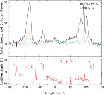
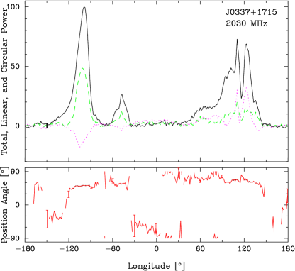
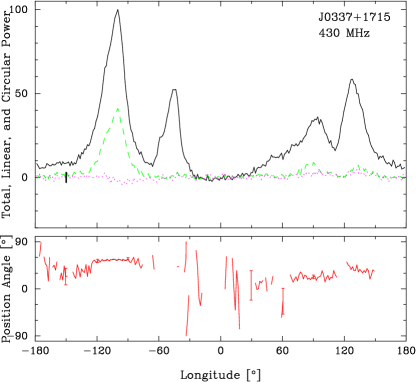
Figure 2.— Arecibo PUPPI profiles of J0337+1715 after Fig. 1 at higher and lower frequencies than the earlier 1391-MHz profile; see Table 1. These show the near absence of evolution with frequency. The profiles, as well as that at 1.4-GHz above, are aligned with the dispersive delay removed.

3. Exploration of the J0337+1715 profile

3.1. The Putative Core Feature and its Width

In slower pulsars, the core component width reflects the angular diameter of the polar cap near the stellar surface, and as such has an intrinsic half-power diameter of $2.45\arcdeg P^{-1/2}$ ($P$ is the stellar rotation period), but the observed width entails a further factor of $\csc\alpha$ (where $\alpha$ is the colatitude of the magnetic axis with respect to the rotation axis). The expected intrinsic width for this 2.73-ms MSP would then be some 47° and the observed width 67.5°, given that $\alpha$ is plausibly 44° (Ransom et al  2014) if the orbital and rotational angular momenta are aligned. In J0337+1715’s profile, the putative core is conflated with the trailing inner conal component over the entire observable band, therefore the core width can only then be estimated. Exploratory modeling of the four profiles in the Appendix suggests a core width of between 60 and 70°, so we have fixed the core width in our modeling at the above expected 67.5° observed value.

3.2. Double Cone Configuration

In slower pulsars, conal components occur in pairs for interior sightline traverses where the sightline impact angle $|\beta|$ is smaller than the conal beam radius $\rho$. Geometrically, these conal component pairs are found to be of two types, inner and outer cones, that have specific (outside, half-power, 1-GHz) radii $\rho$ of $4.33\arcdeg P^{-1/2}$ and $5.75\arcdeg P^{-1/2}$ (ET VIa,b; see VIa eq.(4)). In pulsars where both cones and a core are observed, profiles then have five components, such as in pulsar B1237+25.

We suggest that pulsar J0337+1715’s profile in Fig. 1 may exhibit just these five components as well as a narrow (putative caustic; see below) feature on the outer edge of the trailing inner conal component, and we also model these features in the Appendix. The leading outside (LOC) and inside conal (LIC) components are seen to fall at about –100° and –50° longitude, respectively.

The core is conflated with the trailing conal components (TIC and TOC) at some +100° and +125°, as modeled and better estimated in Table A1. The conal components are asymmetric and the rightmost one has a trailing edge bump. However, the Appendix modeling appears to locate their centers and half widths adequately. The “spike” on the trailing edge of the trailing inner conal feature above 1 GHz deserves special mention, as it seems to resemble the “caustic” features that are seen in some other pulsars. The 1391-MHz polarization-angle (PPA) traverse shows what seems to be a 90° “jump” at about 135° longitude, and earlier ones at about 50° and 100°; if these are resolved, then the PPA seems to rotate rather little under the components as seems possibly the case at the other more depolarized frequencies.

3.3. Quantitative Geometry

Profiles for frequencies both higher and lower than that in Fig. 1 are given in Figure 2. Note that the pulsar’s five components can easily be discerned in these profiles up to 2.8 GHz and down to 430 MHz. The conal features of the 430-MHz profile are broader and appear less well resolved compared to the higher frequency profiles; however, this appears not to be the result of poorer instrumental resolution and scattering. The core is obviously conflated with the trailing inner conal component across all the observations, and this must be taken into account in identifying the structures contributing to the pulsar’s overall profile.

The centers (C), widths (W) and amplitudes (A) of J0337+1715’s components are given in Table A1, where an effort was made to determine these values by fitting methods. However, given the irregular shapes of the components, the fitting errors are small compared to systematic ones of a few degrees. The table thus gives the positions and widths of the conal components so obtained as well as those of the putative “caustic” feature (CC in Table A1) whose center could be fitted within about 1°—and it is satisfying to see that this feature aligns in the high frequency profiles within this latter error. Unsurprisingly, the core component properties are more difficult to estimate in the various profiles, even when taking the widths as fixed at the expected value as shown in the table. We discuss this further below in connection with the A/R analysis where this difficulty is most pertinent.

The properties of the two cones are given in Table LABEL:tab2, where $w_{i}$ and $w_{o}$ are the inner and outer outside, half-power conal widths, computed as the longitude interval between the component-pair centers plus half the sum of their widths. Here we see that the inner and outer conal widths are essentially constant over the observable frequency band. This near constancy of profile dimensions over some three octaves is similar to that observed for other millisecond pulsars where there is little change in the components separations over the total band of observations (e.g., Kondratiev et al  2016).

Here we apply the standard spherical geometric analyses assuming a central sightline traverse (sightline impact angle $\beta$ about 0° as suggested by the relatively constant PPA traverse), that the magnetic latitude $\alpha$ is 44°, and that the emission occurs adjacent to the “last open field lines” (e.g., ET VIa). This analysis is summarized in Table LABEL:tab2, where $\rho_{i}$ and $\rho_{o}$ are the computed conal emission beam radii (to their outside half-power points) per eq.(4) in ET VIa. The emission characteristic heights are then computed assuming bipolarity using eq.(6).

The outside half-power conal radii of about 54° and 75° are of course enormous compared to those found for slow pulsars. However, they are substantially smaller—only about 2/3—what would be expected according to the slow pulsar relationships $4.33\arcdeg P^{-1/2}$ and $5.75\arcdeg P^{-1/2}$ for the outside 3-dB radii of inner and outer cones. The model emission heights of some 53 and 100 km are also correspondingly smaller—less than half of the 120 and 210 km typically seen in the slow pulsar population. However, it is important to recall that these are characteristic emission heights, not physical ones, estimated using the convenient but problematic assumption that the emission occurs adjacent to the “last open” field lines. It will be interesting to compare these heights with the physical emission heights estimated using aberration/retardation (A/R) just below.

Table 2Double Cone Geometry Model for PSR J0337+1715

Freq	$w_{i}$	$\rho_{i}$	$w_{o}$	$\rho_{o}$	$h_{i}$	$h_{o}$
(MHz)	(°)	(°)	(°)	(°)	(km)	(km)
2800	162	54	238	74	52	99
2080	163	54	242	74	53	101
1391	166	55	240	74	53	99
430	163	54	252	76	53	107

Notes: $w_{i}$ and $w_{o}$ are the outside half-power inner and outer conal component widths scaled from Figs. 1 and 2. $\rho_{i}$ and $\rho_{o}$ are the outside half-power conal beam radii computed from ET Paper VIa, eq.(4), and $h_{i}$ and $h_{o}$ are the respective geometric conal emission heights computed from the latter paper’s eq.(6) assuming bipolarity and emission along the polar fluxtube boundary.

Table 3Aberration/Retardation Analysis Results for PSR J0337+1715

Freq/Cone	$\phi^{i}_{l}$	$\phi^{i}_{t}$	$\phi^{i}_{c}$	$\kappa^{i}$	$\rho^{i}$	$h^{i}_{em}$	$s^{i}$
(MHz)	(deg)	(deg)	(deg)	(deg)	(deg)	(km)
2800/II	$-105\pm 3$	$124\pm 4$	$10\pm 5$	$-75\pm 11$	$71.5\pm 1.6$	$86\pm 13$	$0.91\pm 0.07$
2030/II	$-102\pm 3$	$125\pm 4$	$11\pm 5$	$-74\pm 11$	$71.1\pm 1.7$	$84\pm 13$	$0.92\pm 0.07$
1391/II	$-100\pm 3$	$128\pm 4$	$14\pm 5$	$-71\pm 11$	$71.2\pm 1.6$	$81\pm 13$	$0.94\pm 0.07$
430/II	$-103\pm 3$	$129\pm 4$	$13\pm 5$	$-72\pm 11$	$72.2\pm 1.6$	$82\pm 13$	$0.94\pm 0.07$
2800/I	$-51\pm 2$	$98\pm 4$	$24\pm 4$	$-62\pm 11$	$49.5\pm 1.9$	$70\pm 12$	$0.74\pm 0.07$
2030/I	$-49\pm 2$	$97\pm 4$	$24\pm 4$	$-61\pm 11$	$48.9\pm 1.9$	$69\pm 12$	$0.74\pm 0.07$
1391/I	$-47\pm 2$	$99\pm 4$	$26\pm 4$	$-59\pm 11$	$48.9\pm 1.9$	$67\pm 12$	$0.75\pm 0.07$
430/I	$-48\pm 2$	$94\pm 4$	$23\pm 4$	$-62\pm 11$	$47.5\pm 2.0$	$71\pm 13$	$0.71\pm 0.06$

Notes: $\phi^{i}_{l}$ and $\phi^{i}_{t}$ are the leading and trailing conal component positions; $\phi^{i}_{c}$ their centers; $\kappa^{i}$ are the total A/R shifts in longitude as marked by the core component centers; $h^{i}_{em}$ the A/R emission heights computed from eq.(2); and $\rho^{i}$ and $s^{i}$ are the conal radii and emission annuli within the polar fluxtube computed using ET Paper VIa eq.(4) and $\sin(2\rho^{i}/3)\sqrt{R_{lc}/h^{i}}$, respectively.

3.4. Aberration/Retardation Analysis

Here we see that the centers of the outer and inner conal component pairs precede the longitude of the core-component center by some 60° or more—and we propose to interpret this shift as due to aberration/retardation (A/R) to assess whether the results are appropriate and reasonable. A difficulty is determining the position of the core component accurately, given its conflation with the outer conal components. Table A1 below reports the results of modeling the pulsar’s features with Gaussian functions in order to assess the character of this conflation and then estimate the core component’s position and center. Assuming a constant core width at its expected 67.5° value and a constant amplitude in relation to the four conal components, the core center falls close to –85° in each band within about 2°. However, other modeling assumptions might well yield somewhat different values. We therefore propose to take the core center at –85°$\pm$10° in order to incorporate the major range of estimates and uncertainties. Finally, as emphasized above, core components exhibit a predictable width in slow pulsars that reflects both the polar cap geometry and the magnetic colatitude. This is the rationale for holding the core width here to its expected value. If, however, J0337+1715, for whatever reason, had a core that was smaller or larger, then the center would shift by half the difference amount.

Table LABEL:tab3 below gives A/R analyses for the two cones in the four bands. The column values give the peaks of the leading and trailing conal components $\phi_{l}$ and $\phi_{t}$, their center point $\phi_{c}$=($\phi_{t}+\phi_{l}$)/2, and the offsets. The total A/R shift is then given by $\kappa$, which is computed as the longitude interval between the conal centers $\phi_{c}$ and the longitude of the magnetic axis as marked by the core component, or +85° – $\phi_{c}$, and its uncertainty is dominated by the above $\pm$10° in the estimated core position.

The conal radii $\rho$ corresponding to the conal component-pair peak separations are calculated geometrically as in Table LABEL:tab2, and those values are somewhat larger as expected, about 54 and 75°, than tabulated here, given their reference to the outside half-power points rather than the component peaks. This computation is independent of the A/R height determination and is used only to estimate the annuli of the emitting locations $s^{i}$, where 0 lies along the magnetic axis and unity on the polar flux tube boundary. That these values for the outer cone are close to unity tends to support our geometrical model assumption above that its emission regions lie on the periphery of the (dipolar) polar fluxtube; the inner cone is then emitted more to the interior and higher in altitude.

In A/R analysis here per eq.(2) the relation

$$h_{em}=-c\phi_{c}P/360\arcdeg/2$$ (2)

provides a reliable estimate of the emitting region height, subject only to correct interpretation of the core-cone beam structure and determination of the core component’s position as marking the magnetic axis longitude or a region just above it—in any case at a much lower altitude than the conal emission. The resulting physical A/R emission heights for the inner and outer cones are then about 70 km and 85 km, respectively, where the velocity-of-light cylinder distance is $R_{lc}$ (=$cP/2\pi$) of 130 km. We find no significant emission-height differences over the nearly three octaves of observations. This analysis parallels those for slower pulsars in Force & Rankin (2010), Mitra & Rankin (2011), Smith et al  (2013) and most recently Mitra et al  (2016) and are based on BCW as corrected by Dyks et al  (2004).

4. Apparent Core-Cone Beam Structure in Other MSPs

4.1. B1913+16

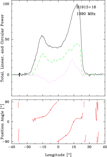
Figure 3.— Arecibo 1.4-GHz Mock-spectrometer profile of B1913+16 from 2012 September 29. The form of this profile differs substantially from those measured earlier (e.g., BCW) due to the star’s precession. This observation was carried out with four Mocks sampling 86-MHz bandwidths and 95 $\mu$sec resolution. The PPAs have been derotated to infinite frequency using the measured $RM$ value above, ionosphere corrected, of +354.4$\pm$0.4 rad-m${}^{2}$.

Table 4Conal Geometry Models for B1913+16, B1953+29 and J1022+1001

Pulsar	$P$	$\alpha$	$\beta$	$w$	$\rho$	$h$
	(ms)	(°)	(°)	(°)	(°)	(km)
B1913+16	59.0	46	4.0	47	17	126
B1953+29	6.1	$>$65	–18	100	44.4	81
J1022+1001	16.4	$\sim$60	$\sim$7	42	20	45

Notes: $P$, $\alpha$ and $\beta$ are the pulsar’s rotation period, magnetic colatitude and sightline impact angle, respectively. The $w$s are the outside half-power conal component widths measured from the fitting of Figs. LABEL:figA3 LABEL:figA4 and LABEL:figA5. The $\rho$s are the outside half-power conal beam radii computed from ET Paper VIa, eq.(4), and the $h$s are the respective geometric conal emission heights computed from the above eq.(6) assuming bipolarity and emission along the polar fluxtube boundary.

The Binary Pulsar B1913+16 has been studied intensively using timing methods, resulting in the identification of gravitational radiation (e.g., Weisberg & Huang 2016) but until recently the pulsar was difficult to study polarimetrically. Moreover, the star precesses causing secular changes in its profile and polarization (e.g., Weisberg & Taylor 2002). However, its early basic profile morphology had been known to be tripartite at 430 MHz and double at 1400 MHz and above. This is just as seen in many slow pulsars, and one of us classified this pulsar as having a core/inner-cone triple (T) profile (ET Paper VIb) on the basis of the 430- and 1400-MHz profiles then recently published by Blaskiewicz et al  (1991; their fig. 17). These profiles show a typical evolution due to the core’s relatively steep spectrum—such that in B1913+16 the core is not resolvable at frequencies above 1 GHz. Key to understanding the central component as being a core is its width, which reflects the angular size of the star’s polar cap at $2.45\arcdeg P^{-1/2}$ or 10° intrinsically and then broader by a factor of $\csc\alpha$ in profile longitude. Our Gaussian fit to the 1990 430-MHz profile in Fig. LABEL:figA3 gives a value of 17$\pm$2° which supports both the core identification and an $\alpha$ value of about 45° as in ET VI (where the 1-GHz width is taken as 14°. This in turn is quite reasonable if the star’s spin and orbital rotations were aligned, but the pulsar’s precession shows that they are not. The star’s changing profile forms at 430 MHz suggest a core/cone beam moving toward and ever less central sightline traverse, greatly complicating models of its emission geometry.

We then take the geometric model in Paper ET VIb, table 4, based on BCWs profiles—at a time when the 430-MHz core was most clearly seen—as close to the mark for our purposes here. Its central sightline traverse makes it insensitive to $\beta$. Similarly, the 430-MHz profile is broader at the conal outside half-power points, but the conal peak separation is nearly constant at about 40° between the two frequencies, so the increased breadth must be intrinsic and the cone thus an inner one. Therefore, we confirm the core/inner-cone geometry of Paper VI.

BCW pioneered the use of A/R for determining pulsar emission heights, and their analysis for B1913+16 is illustrated in their fig. 17. They determined the A/R shift from the PPA steepest gradient point (SG) backward to the center of the conal component pair. Arrows in the figures show these points, and according to their analysis the A/R shift, averaged between the two frequencies, is 12.5°$\pm$ 1.0°, that then corresponds to an emission height of 126$\pm$21 km. This in turn then occurs within a light-cylinder radius of 2820 km.

If the above two points are well identified, the above A/R value follows the method BCW advocated. We can then try to estimate the emission height by two other methods: first, the fits in Fig. LABEL:figA3 clearly show that the core component peak lags the center point between the two conal peaks, and this lag is 1.5° or 0.246 msec or some 37 km in altitude per eq.(1)—that is, the conal emission region appears to be higher than the core region by this amount. Second, the zero-crossing point of antisymmetric circular polarization often marks the longitude of the magnetic axis, and in the B1913+16 profile of Fig. 3 this point falls 6$\pm$1° or some 1.0 msec after the conal center point suggesting a conal emission height of 148$\pm$25 km. As the magnetic axis longitude falls halfway between the oppositely shifted profile and PPA traverse under A/R, the latter result is compatible with BCW’s interpretation and the 37-km shift may represent the height between the core and conal emission regions.

4.2. B1953+29

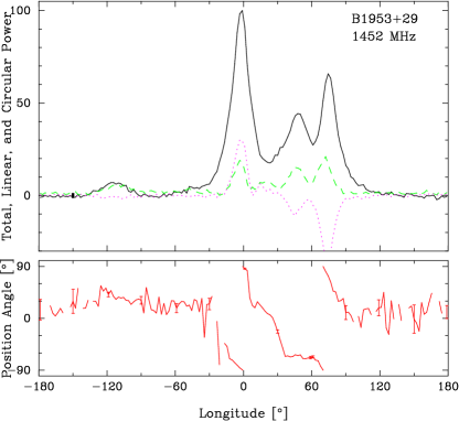
Figure 4.— Arecibo 1.4-GHz Mock-spectrometer profile of B1953+29 from 2013 October 20. This observation was carried out with seven Mocks sampling adjacent 34-MHz bands with a 38 $\mu$sec sampling time. Note what appears to be an interpulse preceding the putative core-cone triple (T) main pulse. We believe this is the first observation to clearly show the pulsar’s PPA traverse and interpulse. The PPAs have been derotated to infinite frequency using its measured RM of +2.9$\pm$0.6 rad-m${}^{2}$ (including some 0.8 rad-m${}^{2}$ in the ionosphere). A further Arecibo observation carried out with PUPPI confirms the profile structure and $RM$ value.

The second millisecond pulsar, B1953+29, aka Boriakoff’s Pulsar (Boriakoff et al  1983) is also a binary pulsar with a 117-day orbit. It has also had little subsequent study as few profiles have been measured in the intervening decades. Profiles and provisional polarimetry at both 430 and 1400 MHz were presented at an NRAO workshop just after the discovery (Boriakoff et al  1984) but not otherwise published, and the polarimetry efforts appearing since (Thorsett & Stinebring 1990; Xilouris et al  1998; Han et al  2009; Gonzalez et al  2011) leave many questions unanswered. The pulsar was difficult to observe polarimetrically, but Arecibo’s L-band Wide feed together with the Mock spectrometers or PUPPI now permit much more sensitive and resolved observations.

Boriakoff et al ’s 430-MHz profile is single, showing only weak inflections from power in conal outriders on both sides of the broad and relatively intense central component. At the higher frequency, however, all three components are visible and distinct. This is just the evolution seen for most conal single (S${}_{t}$) pulsars as first described in Rankin (ETI, ETVIa). No full beamform computation was given for the pulsar in ETVIb because no reliable polarimetry was then available.

Figure 4 shows a recent Arecibo 1452-MHz polarimetric observation conducted with the Mock spectrometers. It is far more sensitive and better resolved than any previously published polarimetry for this important pulsar, and clearly shows its PPA traverse as well as what appears to be a bright interpulse. Again, we have little basis for proceeding with our interpretation of the B1953+29 profile unless its putative core component shows an adequate width reflecting that of the polar cap. For this 6.1-msec pulsar, the intrinsic core width $2.45\arcdeg P^{-1/2}$ [ET VIa, eq.(2)] is expected to be some 31.3°. Fits to the central component discussed in the Appendix give a width of 34.5° with a fitting error of less than a degree. The larger error here, though, is systematic: a Gaussian function may not fit the core feature well and the adjacent overlapping components imply significant correlations. The fitting then indicates a core width which is unlikely to be larger than the fitted value but possibly a little smaller. Thus there is strong indication that this is a core, and that the width reflects a magnetic colatitude—via the $\csc\alpha$ factor—close to orthogonal, that is, some 65° or more. The leading feature (preceding the core by about 163°) would then support a nearly orthogonal geometry if indeed this is an interpulse—and we will make this assumption.

Now we can also see from Figure 4 that the PPA rate is about –3°/°. Following the quantitative geometric analysis of ET VI using the profile dimensions (see the Appendix and Table A2), the results are given in Table LABEL:tab4, where for a magnetic colatitude $\alpha$ of 65° the characteristic emission height would be only some 81 km (rather than the 110-120 km typical of inner-cone characteristic heights of normal pulsars). An A/R analysis of the B1953+29 profile, assuming that the core component is at the longitude of the magnetic axis, results in the conclusion that the conal center precedes the core by 11$\pm$3°, and that in turn corresponds a relative core-cone emission height difference of 27$\pm$5 km within a light-cylinder radius of 293 km.

4.3. J1022+1001

PSR J1022+1001, discovered by Camilo et al  (1996), is a recycled millisecond pulsar with a rotation period of 16 msec. It is in a binary system with an orbital periodicity of 7.8 days. The pulsar has been part of several long term timing programs, but is well known to time poorly. It has been observed over a broad frequency band, (e.g., Dai et al  2015; Noutsos et al  2015), and below 1 GHz its profile is clearly comprised of three prominent components. The underlying PPA traverse has a characteristic S-shaped RVM form with a “kink” under the central component similar that seen in B0329+54 by Mitra et al  (2007), such that the central slope is some 7°/° (Xilouris et al  1998; Stairs et al  1999). Some studies argue that the pulsar exhibits profile changes on short timescales, an effect perhaps similar to mode changing in normal pulsars (see Kramer et al  1999; Ramachandran & Kramer 2003; Hotan et al  2004; and Liu et al  2015). Our three pairs of Arecibo observations at 327 and 1400 MHz also suggest slightly different linear and circular polarization at different times, while confirming the basic profile structures seen in the above papers and the star’s profiles shown here.

In Fig. LABEL:figA5 we show Gaussian component fits to J1022+1001 using profiles from Stairs et al  (1999) (Jodrell Bank profiles downloadable from the European Pulsar Network database). We find that these profiles can be decently fitted with three components, the central one having a width of 17° at 610 MHz and 14° at 410 MHz, roughly close to the polar cap size of 19°. In these fits the location and width of the leading component are highly correlated and cannot be constrained very well, with some effect also on the central component. This said, the effect of A/R in terms of the core center lagging the center of the overall profile is clearly seen in this pulsar. The magnitude of this lag is about 6.5° at 410 MHz and 7° at 610 MHz, where we find the center of the overall profile based on the outer Gaussian-fitted component half-power points in Table A2. These estimates place the conal emission at about 20 km above the core emission.

In a short communication Mitra & Seiradakis (2004) used an A/R model to estimate the emission height across the pulse. They argued that the pulsar could be interpreted in terms of a central core and a conal component pair as shown in their fig. 2. They found a slight difference in emission height between the core and conal emission, which then had the effect due to A/R of inserting a kink in the PPA traverse similar to what is observed. For this to happen they suggest that the core emission originates closer to the neutron star surface, and the conal emission region is then about 25 km above that of the core emission, similar to estimates obtained from the profile analysis mentioned above.

5. Summary of Observational Results

MSP J0337+1715 apparently provides a rare opportunity to study a core/double-cone emission beam configuration in the recycled and relatively weak magnetic field system of a millisecond pulsar. Slow pulsars with five-component profiles showing the core and both conal beams are unusual—because our sightline must pass close to the magnetic axis to encounter the core and resolve the inner cone—but such stars exhibit the most complex beamforms that pulsars normally seem capable of producing.

The conal dimensions of J0337+1715 and A/R analysis provide a novel and consistent picture of the emission regions in this MSP. The A/R analysis argues that the inner conal emission is generated at a height of some 70 km and the outer cone then at about 85 km, and adjustment of the quantitative geometry for the estimated $s_{L}$ values provides roughly compatible emission heights. No evidence of conal spreading is seen over the nearly three octave band of observations, again suggesting that all the emission is produced within a narrow range of heights.

Questions have remained about whether MSPs radiate in beamforms similar to those of slower pulsars. When putative core components have been seen in MSPs—as in the roughly five-componented profiles of J0437–4715—they are usually narrower than the polar-cap angular diameter and thus cannot be core emission features in the manner known from the slow pulsar population. This might be because MSP magnetic dipoles are not centered in the star, which in turn might result from the field destruction during their accretional spinup phase (e.g., Ruderman 1991). Or conversely, perhaps in J0337+1715 this field destruction was more orderly or less disruptive than in many other MSPs.

Core/cone beam structure had heretofore been identified in a few MSPs—B1913+16, B1953+29 and J1022+1001—and not systematically assessed in these until recently because the available polarimetry made quantitative geometric modeling difficult and inconclusive. Here we have been able to carry out such analyses that argue strongly for core/cone structure in these three other MSPs. In each case we find core widths that are compatible with the full angular size of their (dipolar) polar caps at the surface. We further find characteristic emission heights for these pulsars that are all smaller or much smaller than expected for the inner cones of normal pulsars. A/R analyses then provide more physical emission heights: For B1913+16, a 59-ms MSP with the largest light-cylinder of 2820 km, its properties are most like those of slow pulsar inner cones. For each of the other three, however, with much faster rotations and smaller magnetospheres, both the quantitative geometry and A/R analyses indicate radio emission from lower altitudes of only a few stellar radii.

These results can embolden us to recognize core/cone structure in other MSPs, classify them and study their emission geometry quantitatively in order to determine if, in fact, some few other core/cone profiles can be recognized among the many MSPs with inscrutable ones. These results underscore that while the few MSPs here seem to exhibit such structure, many or most appear not to. Thus these results may begin to provide a foundation for exploring the consequences of accretional magnetic field destruction during MSP spinup. It may well be that orderly core/cone beam structure signals and depends on a nearly dipolar magnetic field configuration at the height of the radio-emission regions (Rankin et al  2017). Therefore, for reasons to be learned in the future, some MSPs may be able to retain a sufficiently dominant dipolar magnetic field in their radio emission regions despite its dramatic weakening by accretion—whereas, most other MSPs apparently do not.

Table 5Summary of plasma properties for MSP radiation.

Pulsar	P	$\dot{P}$	Beamform	$\nu_{obs}$	h	$\nu_{B}$	$\nu_{p}$	$\nu_{cr}$	$R$	R${}_{lc}$
	(ms)	(10${}^{-20}$ s/s)		(GHz)	(km)	(GHz)	(GHz)	(GHz)		(km)
J0337+1715	2.732	1.76	Inner Cone	1.4	69	19	15$-$146	11$-$87	0.53	130
			Outer Cone	1.4	83	11	11$-$111	10$-$79	0.64	130
B1913+16	59.0	86	Inner Cone	1.4	126	101	7$-$73	2$-$14	0.04	2817
B1953+19	6.13	2.97	Inner Cone	1.4	27	614	55$-$555	12$-$93	0.09	293
					81	23	11$-$107	7$-$54	0.28	293
J1022+1001	16.4	4.3	Inner Cone	1.4	25	1530	53$-$535	7$-$59	0.03	786
					45	262	22$-$221	5$-$44	0.06	786

Notes: The frequency $\nu_{B}$ is the cyclotron frequency estimated for $\gamma_{s}=200$, frequency $\nu_{p}$ estimated for $\gamma_{s}=200$ and two values of $\kappa=100,10^{4}$, the cyclotron frequency estimated for two values of $\Gamma_{s}=300,600$. Italicized values follow from the geometric model (characteristic) heights in Table LABEL:tab4.