\thankstext

e1e-mail: buccioni@physik.uzh.ch \thankstexte2e-mail: pozzorin@physik.uzh.ch \thankstexte3e-mail: zoller@physik.uzh.ch

11institutetext: Physik-Institut, Universität Zürich, CH-8057 Zürich, Switzerland

On-the-fly reduction of open loops

Federico Buccioni\thanksrefe1,inst1    Stefano Pozzorini\thanksrefe2,inst1    and Max Zoller\thanksrefe3,inst1
(Received: date / Revised version: date)
Abstract

Building on the open-loop algorithm we introduce a new method for the automated construction of one-loop amplitudes and their reduction to scalar integrals. The key idea is that the factorisation of one-loop integrands in a product of loop segments makes it possible to perform various operations on-the-fly while constructing the integrand. Reducing the integrand on-the-fly, after each segment multiplication, the construction of loop diagrams and their reduction are unified in a single numerical recursion. In this way we entirely avoid objects with high tensor rank, thereby reducing the complexity of the calculations in a drastic way. Thanks to the on-the-fly approach, which is applied also to helicity summation and for the merging of different diagrams, the speed of the original open-loop algorithm can be further augmented in a very significant way. Moreover, addressing spurious singularities of the employed reduction identities by means of simple expansions in rank-two Gram determinants, we achieve a remarkably high level of numerical stability. These features of the new algorithm, which will be made publicly available in a forthcoming release of the OpenLoops program, are particularly attractive for NLO multi-leg and NNLO real–virtual calculations.

pacs:
02.70.-c, 12.15.Lk, 12.38.-t, 12.38.Bx
journal: Eur. Phys. J. C

1 Introduction

The continuous improvement of statistics and experimental systematics at the Large Hadron Collider (LHC) permits to challenge the Standard Model of particle physics at steadily increasing levels of energy and precision. In this context, the uncertainty of theoretical predictions starts playing a critical role in many areas of the physics program of the LHC, providing strong motivation for developing new techniques that make it possible to push theoretical calculations towards more complex processes and higher perturbative orders.

In the last decade, the advent of new powerful methods for the calculation of one-loop scattering amplitudes Britto:2004nc ; delAguila:2004nf ; Bern:2005cq ; Denner:2005nn ; Ossola:2006us ; Forde:2007mi ; Giele:2008ve ; vanHameren:2009vq ; Cascioli:2011va has opened the door to the automation of next-to-leading order (NLO) calculations. Nowadays, one-loop calculations are supported by a number of highly automated tools Ossola:2007ax ; Berger:2008sj ; vanHameren:2009dr ; Hirschi:2011pa ; Mastrolia:2010nb ; Badger:2012pg ; hepforge ; Cullen:2014yla ; Peraro:2014cba ; Denner:2016kdg ; Actis:2016mpe that provide the key to achieve NLO precision in the context of multi-purpose Monte Carlo generators Gleisberg:2008ta ; Alioli:2010xd ; Bevilacqua:2011xh ; Alwall:2014hca ; Sjostrand:2014zea ; Weiss:2015npa ; Bellm:2015jjp . This recent progress has enabled NLO calculations for a huge number of processes and has extended their reach up to multi-particle final states of unprecedented complexity Bern:2013gka ; Badger:2013yda ; Bevilacqua:2015qha ; Hoche:2016elu ; Denner:2016wet . Nevertheless, in various cases the technical limitations of one-loop generators still represent a serious bottleneck or even a show stopper. These issues can be encountered in processes with many final-state particles and for kinematic configurations with two or more widely separated scales. An important example is given by the real–virtual contributions to next-to-next-to leading order (NNLO) calculations, which require very fast and highly stable one-loop amplitudes in deeply infrared regions of phase space.

Motivated by these considerations, in this paper we introduce a new method that leads to very significant efficiency and stability improvements in the construction of one-loop amplitudes. This new method builds on OpenLoops Cascioli:2011va ; hepforge , a fully automated framework for the automated generation of scattering amplitudes in the Standard Model. The original implementation of the open-loop approach Cascioli:2011va ; hepforge supports NLO QCD Cascioli:2013gfa ; Cascioli:2013era ; Cascioli:2013wga ; Hoeche:2014qda ; Hoeche:2014rya ; Jezo:2016ujg ; Hoche:2016elu ; Nejad:2016bci as well as NLO EW Kallweit:2014xda ; Kallweit:2015dum ; Kallweit:2017khh ; Lindert:2017olm ; Granata:2017iod calculations and is interfaced to various multi-purpose Monte Carlo tools. The OpenLoops program is also part of Matrix Wiesemann:2016eiw and has already been applied to several NNLO calculations Grazzini:2013bna ; Cascioli:2014yka ; Gehrmann:2014fva ; Grazzini:2015nwa ; Grazzini:2015wpa ; Grazzini:2015hta ; Grazzini:2016swo ; Grazzini:2016ctr ; deFlorian:2016uhr ; Grazzini:2017ckn . The essence of the open-loop method Cascioli:2011va consists of a numerical recursion that generates cut-open loop diagrams, called open loops, by multiplying, one after the other, the various building blocks that are connected through loop propagators. More precisely, the construction of N𝑁N-point loop integrands is organised through the factorisation of N𝑁N loop segments, which consist each of a loop propagator and a corresponding external subtree. Segment multiplications are implemented through process-independent numerical routines that correspond to the Feynman rules of the model at hand. This type of recursion was first proposed in the context of off-shell recurrence relations for colour-ordered gluon-scattering amplitudes vanHameren:2009vq . Thanks to a tensorial representation that retains the loop-momentum dependence of all building blocks, this approach can be used in combination with reduction techniques based on tensor integrals Denner:2005nn or with the OPP reduction method Ossola:2006us , resulting in both cases in very fast computer code Cascioli:2011va .

The new method presented in this paper exploits the factorised structure of the open-loop representation in a completely new way. The key idea is that certain operations, which are usually done when all building blocks of Feynman diagrams have been assembled, can be anticipated and performed on-the-fly during the construction of the diagrams. Exploiting the factorised structure of the integrands, this on-the-fly approach permits to perform various types of operations at a much lower level of complexity, thereby boosting their efficiency. As we will show, it can be exploited in order to factorise helicity summations as well as the sums over different Feynman diagrams that share the same one-loop topology. Moreover, based on the integrand reduction method by del Aguila and Pittau delAguila:2004nf , we will introduce an on-the-fly technique for the reduction of open loops. In this way, we will promote OpenLoops to an algorithm that combines the construction and the reduction of loop amplitudes in a unified numerical recursion. A notable feature of this approach is that it permits to avoid high-rank objects at any stage of the calculations. More precisely, tensor integrals are always kept at rank two or lower, thereby reducing the computational complexity in a dramatic way.

The on-the-fly technique leads to very significant improvements of CPU efficiency. For what concerns numerical stability, in order to avoid severe instabilities that result from squared inverse Gram determinants in the reduction identities of delAguila:2004nf , we present a method that isolates such instabilities in certain triangle topologies and circumvents them via analytic expansions in the limit of small Gram determinants. In this way we obtain the first integrand-reduction algorithm that is essentially free from Gram-determinant instabilities. The achieved level of stability in double precision is competitive with the most sophisticated tools on the market Denner:2016kdg and with public implementations of OPP reduction in quadruple precision.

The paper is organized as follows. In Section 2 we review the original open-loop method. The on-the-fly approach is introduced in Section 3 for the case of helicity sums and for the merging of topologically equivalent open loops. In Section 4 the on-the-fly approach is generalised to the reduction of open loops. Details on the employed integrand-reduction identities and our treatment of Gram-determinant instabilities are discussed in Section 5. The entire algorithm and its implementation are outlined in Section 6, where we also present technical studies on the CPU performance and numerical stability. Our conclusions are presented in Section 7, and A deals with low-rank integrals that remain to be solved at the end of the on-the-fly recursion.

2 The open-loop method

In this section we review the original open-loop method Cascioli:2011va , which is implemented in the publicly available OpenLoops 1 program hepforge . At variance with the original publication Cascioli:2011va , here we refine various aspects of the notation and we adopt a particular perspective that sets the stage for the new methods introduced in Sections 35. These new techniques are going to become publicly available in the OpenLoops 2 release.

2.1 Helicity and colour bookkeeping

The task carried out by the open-loop algorithm is the calculation of the tree-level and one-loop contributions to the scattering probability density,

𝒲treesubscript𝒲tree\displaystyle\mathcal{W}_{\mathrm{tree}} =\displaystyle= hcol|0(h)|2,subscriptsubscriptcolsuperscriptsubscript02\displaystyle\sum_{h}\sum_{\mathrm{col}}|\mathcal{M}_{0}(h)|^{2},
𝒲1loopsubscript𝒲1loop\displaystyle\mathcal{W}_{\mathrm{1-loop}} =\displaystyle= hcol2Re[0(h)1(h)],subscriptsubscriptcol2Redelimited-[]superscriptsubscript0subscript1\displaystyle\sum_{h}\sum_{\mathrm{col}}2\,\mathrm{Re}\Big{[}\mathcal{M}_{0}^{*}(h)\mathcal{M}_{1}(h)\Big{]}, (1)

or the squared one-loop contribution

𝒲1loop2=hcol|1(h)|2,subscript𝒲1superscriptloop2subscriptsubscriptcolsuperscriptsubscript12\displaystyle\mathcal{W}_{\mathrm{1-loop}^{2}}=\sum_{h}\sum_{\mathrm{col}}|\mathcal{M}_{1}(h)|^{2}, (2)

for loop-induced processes. The polarised matrix elements 0(h)subscript0\mathcal{M}_{0}(h) and 1(h)subscript1\mathcal{M}_{1}(h) should be understood as generic tree and one-loop amplitudes, in the sense that the techniques presented in this paper are applicable to any renormalisable theory, including the QCD and electroweak sectors of the Standard Model, as well as BSM theories. The sums in (2.1)(2) run over all helicity and colour degrees of freedom of the scattering particles. While colour indices are kept implicit, the helicity dependence is characterised by a single index hh, which corresponds to the global helicity configuration of the event, as described below.

Scattering amplitudes are computed as sums of Feynman diagrams,

0(h)subscript0\displaystyle\mathcal{M}_{0}(h) =\displaystyle= Ωtree0(,h),subscriptsubscriptΩtreesubscript0\displaystyle\sum_{\mathcal{I}\in\Omega_{\mathrm{tree}}}\mathcal{M}_{0}(\mathcal{I},h),
1(h)subscript1\displaystyle\mathcal{M}_{1}(h) =\displaystyle= Ω1loop1(,h),subscriptsubscriptΩ1loopsubscript1\displaystyle\sum_{\mathcal{I}\in\Omega_{\mathrm{1-loop}}}\mathcal{M}_{1}(\mathcal{I},h),\qquad (3)

where ΩtreesubscriptΩtree\Omega_{\mathrm{tree}} and Ω1loopsubscriptΩ1loop\Omega_{\mathrm{1-loop}} stand for the sets of tree and one-loop diagrams. Each tree and one-loop diagram can be factored into a colour factor 𝒞()𝒞\mathcal{C}(\mathcal{I}) and a colour-stripped diagram amplitude,111Quartic gluon couplings involve three independent colour structures. Thus each diagram involving k𝑘k quartic couplings needs to be split into 3ksuperscript3𝑘3^{k} contributions of type (4) that are effectively handled as separate diagrams.

L(,h)=𝒞()𝒜L(,h),subscript𝐿𝒞subscript𝒜𝐿\displaystyle\mathcal{M}_{L}(\mathcal{I},h)=\mathcal{C}(\mathcal{I})\,\mathcal{A}_{L}(\mathcal{I},h), (4)

for L=0,1𝐿01L=0,1. The colour-stripped amplitudes 𝒜L(,h)subscript𝒜𝐿\mathcal{A}_{L}(\mathcal{I},h) are the main source of complexity. In the open-loop approach, their calculation is addressed with numerical recursions as described in Sections 2.22.4. For what concerns colour factors, exploiting the factorisation properties (4), all relevant operations can be reduced to the calculation of colour-summed interference terms of the form

𝒦(a,b)=col𝒞(a)𝒞(b),𝒦subscript𝑎subscript𝑏subscriptcolsuperscript𝒞subscript𝑎𝒞subscript𝑏\displaystyle\mathcal{K}(\mathcal{I}_{a},\mathcal{I}_{b})=\sum_{\mathrm{col}}\,\mbox{$\mathcal{C}(\mathcal{I}_{a})$}^{*}\,\mathcal{C}(\mathcal{I}_{b}), (5)

which appear in the calculation of the scattering probabilities (2.1)-(2). This task must be addressed only once per process. It is handled by algebraically reducing all 𝒞()𝒞\mathcal{C}(\mathcal{I}) to a standard basis {𝒞i}subscript𝒞𝑖\{\mathcal{C}_{i}\} and relating the terms (5) to the interference matrix Bredenstein:2010rs ; Cascioli:2011va

𝒦ij=col𝒞i𝒞j.subscript𝒦𝑖𝑗subscriptcolsuperscriptsubscript𝒞𝑖subscript𝒞𝑗\displaystyle\mathcal{K}_{ij}=\sum_{\mathrm{col}}\,\mbox{$\mathcal{C}_{i}$}^{*}\,\mathcal{C}_{j}. (6)

In OpenLoops we use a basis where all colour factors are expressed through products and traces of the SU(3) generators Tijasubscriptsuperscript𝑇𝑎𝑖𝑗T^{a}_{ij} in the fundamental representation.

For the bookkeeping of external momenta and helicities in a process with Npsubscript𝑁pN_{\mathrm{p}} scattering particles we introduce the set of particle indices

={1,2,,Np}.12subscript𝑁p\displaystyle\mathcal{E}=\{1,2,\dots,N_{\mathrm{p}}\}. (7)

To characterise the helicity configurations s𝑠s of individual particles we use labels

λi={ 1,3for fermions withs=1/2,1/2 1,2,3for gauge bosons withs=1,0,1 0for scalars withs=0subscript𝜆𝑖cases13for fermions with𝑠1212123for gauge bosons with𝑠101 0for scalars with𝑠0\displaystyle\lambda_{i}=\begin{cases}\;1,3&\mbox{for fermions with}\,s=-1/2,1/2\\[5.69054pt] \;1,2,3&\mbox{for gauge bosons with}\,s=-1,0,1\\[5.69054pt] \;0&\mbox{for scalars with}\,s=0\end{cases} (8)

ifor-all𝑖\forall\;i\in\mathcal{E}. The configuration λi=0subscript𝜆𝑖0\lambda_{i}=0 will also be used to characterise unpolarised particles, i.e. fermions or gauge bosons whose helicity is still unassigned or has already been summed over. Since a particle can have up to four different helicity states, it is convenient to adopt a helicity numbering scheme based on the labels

h¯i=λi 4i1,subscript¯𝑖subscript𝜆𝑖superscript4𝑖1\displaystyle\bar{h}_{i}=\lambda_{i}\,4^{i-1}, (9)

which correspond to a quaternary number with λi{0,1,2,3}subscript𝜆𝑖0123\lambda_{i}\in\{0,1,2,3\} as ithsuperscript𝑖thi^{\mathrm{th}}-last digit and all other digits equal to zero. In this way, the helicity configurations (λ1,,λNp)subscript𝜆1subscript𝜆subscript𝑁p(\lambda_{1},\dots,\lambda_{N_{\mathrm{p}}}) of the full event can be uniquely identified with the label

h=h¯1++h¯Np,subscript¯1subscript¯subscript𝑁p\displaystyle h=\bar{h}_{1}+\dots+\bar{h}_{N_{\mathrm{p}}}, (10)

which corresponds to a quaternary number of Npsubscript𝑁pN_{\mathrm{p}} digits, each of which describes the helicity of a particular external particle. Let us also introduce the single-particle helicity spaces, ¯ih¯isubscript¯𝑖subscript¯𝑖\mathcal{\bar{H}}_{i}\ni\bar{h}_{i}, defined as

¯i={{λi 4i1|λi=1,3}for fermions or mass-less gauge bosons,{λi 4i1|λi=1,2,3}for massivegauge bosons,{0}for scalars,subscript¯𝑖casesconditional-setsubscript𝜆𝑖superscript4𝑖1subscript𝜆𝑖13for fermions or mass-otherwiseless gauge bosons,conditional-setsubscript𝜆𝑖superscript4𝑖1subscript𝜆𝑖123for massiveotherwisegauge bosons,0for scalars,\displaystyle\mathcal{\bar{H}}_{i}=\begin{cases}\;\{\lambda_{i}\,4^{i-1}|\lambda_{i}=1,3\}&\;\mbox{for fermions or mass-}\\ &\;\mbox{less gauge bosons,}\\[5.69054pt] \;\{\lambda_{i}\,4^{i-1}|\lambda_{i}=1,2,3\}&\;\mbox{for massive}\\ &\;\mbox{gauge bosons,}\\[5.69054pt] \;\{0\}&\;\mbox{for scalars,}\end{cases} (11)

where we do not include unpolarised states. Finally, the global helicity space for the full set of scattering particles, h\mathcal{H}\ni h, is defined as

=¯1¯Np,tensor-productsubscript¯1subscript¯subscript𝑁p\displaystyle\mathcal{H}=\mathcal{\bar{H}}_{1}\otimes\dots\otimes\mathcal{\bar{H}}_{N_{\mathrm{p}}}, (12)

where the product is understood as 𝒜={a+b|a𝒜,b}tensor-product𝒜conditional-set𝑎𝑏formulae-sequence𝑎𝒜𝑏\mathcal{A}\otimes\mathcal{B}=\{a+b|a\in\mathcal{A},b\in\mathcal{B}\}.

2.2 Tree amplitudes

At tree level, each colour-stripped Feynman diagram is constructed by contracting two so-called subtrees, which arise by cutting the diagram in two pieces in correspondence of an internal propagator,

𝒜0(,h)=[Uncaptioned image]subscript𝒜0[Uncaptioned image]\displaystyle\mathcal{A}_{0}(\mathcal{I},h)\;=\;\;\vbox{\hbox{\scalebox{1.0}{\includegraphics[width=113.81102pt]{diaTreeA}}}} (13)

A generic subtree wasubscript𝑤𝑎w_{a} corresponds to the part of a certain Feynman diagram that connects an internal off-shell line with outgoing momentum kasubscript𝑘𝑎k_{a} to a subset of external particles,

a={αa1,,αana}.subscript𝑎subscript𝛼𝑎1subscript𝛼𝑎subscript𝑛𝑎\displaystyle\mathcal{E}_{a}=\{\alpha_{a1},\dots,\alpha_{an_{a}}\}\subset\mathcal{E}. (14)

In the numbering scheme (9)(10), the helicity configurations of a subtree are labeled

ha=h¯αa1++h¯αana,subscript𝑎subscript¯subscript𝛼𝑎1subscript¯subscript𝛼𝑎subscript𝑛𝑎\displaystyle h_{a}=\bar{h}_{\alpha_{a1}}+\dots+\bar{h}_{\alpha_{an_{a}}}, (15)

and the corresponding helicity space, ahasubscript𝑎subscript𝑎\mathcal{H}_{a}\ni h_{a}, is defined as

a=¯αa1¯αana.subscript𝑎tensor-productsubscript¯subscript𝛼𝑎1subscript¯subscript𝛼𝑎subscript𝑛𝑎\displaystyle\mathcal{H}_{a}=\mathcal{\bar{H}}_{\alpha_{a1}}\otimes\dots\otimes\mathcal{\bar{H}}_{\alpha_{an_{a}}}. (16)

Subtrees are represented as complex n𝑛n-tuples, waσa(ka,ha)subscriptsuperscript𝑤subscript𝜎𝑎𝑎subscript𝑘𝑎subscript𝑎w^{\sigma_{a}}_{a}(k_{a},h_{a}), where σasubscript𝜎𝑎\sigma_{a} is the spinor or Lorentz index of the cut line. With this notation, the contraction (13) takes the form

𝒜0(,h)=waσa(ka,ha)δσaσbw~bσb(kb,hb),subscript𝒜0subscriptsuperscript𝑤subscript𝜎𝑎𝑎subscript𝑘𝑎subscript𝑎subscript𝛿subscript𝜎𝑎subscript𝜎𝑏subscriptsuperscript~𝑤subscript𝜎𝑏𝑏subscript𝑘𝑏subscript𝑏\displaystyle\mathcal{A}_{0}(\mathcal{I},h)\;=\;\;w^{\sigma_{a}}_{a}(k_{a},h_{a})\,\delta_{\sigma_{a}\sigma_{b}}\widetilde{w}^{\sigma_{b}}_{b}(k_{b},h_{b}), (17)

where kb=kasubscript𝑘𝑏subscript𝑘𝑎k_{b}=-k_{a}, h=ha+hbsubscript𝑎subscript𝑏h=h_{a}+h_{b}, and summation over repeated indices is implicitly understood. The propagator associated with the cut line is included only in the subtree wasubscript𝑤𝑎w_{a} and not in w~bsubscript~𝑤𝑏\widetilde{w}_{b}.

Subtrees are constructed by means of a numerical recursion that starts from the external wave functions and recursively merges subtrees by attaching their off-shell lines to the vertices that occur in the various tree diagrams. A recursion step for the case of a generic three-particle vertex is depicted222To draw Feynman diagrams we use Axodraw Vermaseren:1994je . in Fig. 1. Its algebraic form reads

waσa(ka,ha)=Xσbσcσa(kb,kc)ka2ma2wbσb(kb,hb)wcσc(kc,hc),subscriptsuperscript𝑤subscript𝜎𝑎𝑎subscript𝑘𝑎subscript𝑎superscriptsubscript𝑋subscript𝜎𝑏subscript𝜎𝑐subscript𝜎𝑎subscript𝑘𝑏subscript𝑘𝑐superscriptsubscript𝑘𝑎2superscriptsubscript𝑚𝑎2subscriptsuperscript𝑤subscript𝜎𝑏𝑏subscript𝑘𝑏subscript𝑏subscriptsuperscript𝑤subscript𝜎𝑐𝑐subscript𝑘𝑐subscript𝑐\displaystyle w^{\sigma_{a}}_{a}(k_{a},h_{a})=\frac{X_{\sigma_{b}\sigma_{c}}^{\sigma_{a}}(k_{b},k_{c})}{k_{a}^{2}-m_{a}^{2}}\;w^{\sigma_{b}}_{b}(k_{b},h_{b})\;w^{\sigma_{c}}_{c}(k_{c},h_{c}){},

where the tensor Xσbσcσasuperscriptsubscript𝑋subscript𝜎𝑏subscript𝜎𝑐subscript𝜎𝑎X_{\sigma_{b}\sigma_{c}}^{\sigma_{a}} describes the vertex that connects wbsubscript𝑤𝑏w_{b} and wcsubscript𝑤𝑐w_{c} to wasubscript𝑤𝑎w_{a}, as well as the numerator of the propagator that connects to wasubscript𝑤𝑎w_{a}. The related denominator, (ka2ma2)superscriptsubscript𝑘𝑎2superscriptsubscript𝑚𝑎2(k_{a}^{2}-m_{a}^{2}), appears explicitly in (2.2).

waσa(ka,ha)=Refer to captionsubscriptsuperscript𝑤subscript𝜎𝑎𝑎subscript𝑘𝑎subscript𝑎Refer to caption\displaystyle w^{\sigma_{a}}_{a}(k_{a},h_{a})\;=\;\;\vbox{\hbox{\scalebox{1.0}{\includegraphics[width=170.71652pt]{diaTreeB}}}}
Figure 1: Diagrammatic representation of a subtree and its numerical construction through the recurrence relation (2.2). The outgoing momentum kasubscript𝑘𝑎k_{a} and the spin or Lorentz index σasubscript𝜎𝑎\sigma_{a} are associated with the off-shell internal line, which is shown explicitly, while the on-shell external particles with helicity hasubscript𝑎h_{a} are implicitly understood.

The momentum of the resulting subtree is ka=kb+kcsubscript𝑘𝑎subscript𝑘𝑏subscript𝑘𝑐k_{a}=k_{b}+k_{c} and its helicity is ha=hb+hcsubscript𝑎subscript𝑏subscript𝑐h_{a}=h_{b}+h_{c}. Each recursion step must be repeated for all independent helicity configuration haa=bcsubscript𝑎subscript𝑎tensor-productsubscript𝑏subscript𝑐h_{a}\in\mathcal{H}_{a}=\mathcal{H}_{b}\otimes\mathcal{H}_{c}. The corresponding recursion step for quartic vertices reads

waσa(ka,ha)subscriptsuperscript𝑤subscript𝜎𝑎𝑎subscript𝑘𝑎subscript𝑎\displaystyle w^{\sigma_{a}}_{a}(k_{a},h_{a}) =\displaystyle= Xσbσcσdσa(kb,kc,kd)ka2ma2wbσb(kb,hb)superscriptsubscript𝑋subscript𝜎𝑏subscript𝜎𝑐subscript𝜎𝑑subscript𝜎𝑎subscript𝑘𝑏subscript𝑘𝑐subscript𝑘𝑑superscriptsubscript𝑘𝑎2superscriptsubscript𝑚𝑎2subscriptsuperscript𝑤subscript𝜎𝑏𝑏subscript𝑘𝑏subscript𝑏\displaystyle\frac{X_{\sigma_{b}\sigma_{c}\sigma_{d}}^{\sigma_{a}}(k_{b},k_{c},k_{d})}{k_{a}^{2}-m_{a}^{2}}\;w^{\sigma_{b}}_{b}(k_{b},h_{b})\; (19)
×\displaystyle\times wcσc(kc,hc)wdσd(kd,hd).subscriptsuperscript𝑤subscript𝜎𝑐𝑐subscript𝑘𝑐subscript𝑐subscriptsuperscript𝑤subscript𝜎𝑑𝑑subscript𝑘𝑑subscript𝑑\displaystyle w^{\sigma_{c}}_{c}(k_{c},h_{c}){}\;w^{\sigma_{d}}_{d}(k_{d},h_{d}).

The recursion ends when all off-shell propagators that have been cut in the beginning can be reconnected, such as to obtain the colour-stripped amplitudes (17) for the full set of tree diagrams.

Note that (2.2)(19) are analogous to Berends–Giele recurrence relations for off-shell currents Berends:1987me . However, while each subtree corresponds to a single topology, off-shell currents incorporate all possible subtrees associated with a certain internal line. The inefficiency due to the usage of individual subtrees is compensated, especially at one-loop level, by the optimisation opportunities that result from the colour-factorisation identities (4) and from the fact that each subtree can occur in multiple Feynman diagrams at tree and loop level.

2.3 One-loop amplitudes

The amplitude of a colour-stripped N𝑁N-point one-loop diagram, Nsubscript𝑁\mathcal{I}_{N}, has the general form

𝒜¯1(N,h)subscript¯𝒜1subscript𝑁\displaystyle\bar{\mathcal{A}}_{1}(\mathcal{I}_{N},h) =\displaystyle= [Uncaptioned image]=[Uncaptioned image]absent\displaystyle\quad\vbox{\hbox{\scalebox{1.0}{\includegraphics[height=93.32515pt]{diaClosedLoop}}}}\;= (20)
=\displaystyle= dDq¯Tr[𝒩¯(N,q¯,h)]D¯0D¯1D¯N1.superscriptd𝐷¯𝑞Trdelimited-[]¯𝒩subscript𝑁¯𝑞subscript¯𝐷0subscript¯𝐷1subscript¯𝐷𝑁1\displaystyle\int\!\mathrm{d}^{D}\!\bar{q}\,\frac{\mathrm{Tr}\Big{[}\bar{\mathcal{N}}(\mathcal{I}_{N},\bar{q},h)\Big{]}}{\bar{D}_{0}\bar{D}_{1}\cdots\bar{D}_{N-1}}\,.

Symbols carrying a bar denote quantities in D=42ε𝐷42𝜀D=4-2\varepsilon dimensions, and for the loop momentum q¯¯𝑞\bar{q} we adopt the decomposition

q¯=q+q~,¯𝑞𝑞~𝑞\displaystyle\bar{q}=q+\tilde{q}, (21)

where q𝑞q and q~~𝑞\tilde{q} denote its four-dimensional and (D4)𝐷4(D-4)-dimensional parts, respectively. The denominators read

D¯i=(q¯+pi)2mi2,pi=j=1ikj,formulae-sequencesubscript¯𝐷𝑖superscript¯𝑞subscript𝑝𝑖2superscriptsubscript𝑚𝑖2subscript𝑝𝑖superscriptsubscript𝑗1𝑖subscript𝑘𝑗\displaystyle\bar{D}_{i}=(\bar{q}+p_{i})^{2}-m_{i}^{2}\,,\;\,\;\,\;p_{i}=\sum_{j=1}^{i}k_{j}{}, (22)

where kjsubscript𝑘𝑗k_{j} is the external momentum flowing into the loop at the jthsuperscript𝑗thj^{\mathrm{th}} loop vertex. Internal momenta are chosen such that p0=pN=0subscript𝑝0subscript𝑝𝑁0p_{0}=p_{N}=0, i.e. the momentum flowing through the D¯0=D¯Nsubscript¯𝐷0subscript¯𝐷𝑁\bar{D}_{0}=\bar{D}_{N} propagator is q¯¯𝑞\bar{q}. The one-loop diagram Nsubscript𝑁\mathcal{I}_{N} in (20) can be regarded as a sequence of loop segments,

N={𝒮1,𝒮2,,𝒮N},subscript𝑁subscript𝒮1subscript𝒮2subscript𝒮𝑁\displaystyle\mathcal{I}_{N}=\{\mathcal{S}_{1},\mathcal{S}_{2},\ldots,\mathcal{S}_{N}\}, (23)

where the segment 𝒮isubscript𝒮𝑖\mathcal{S}_{i} consists of a subtree wisubscript𝑤𝑖w_{i} that involves a certain set isubscript𝑖\mathcal{E}_{i} of external particles and is connected to the ithsuperscript𝑖thi^{\mathrm{th}} loop vertex, visubscript𝑣𝑖v_{i}, and to the adjacent loop propagator associated with D¯isubscript¯𝐷𝑖\bar{D}_{i}. Segments associated to a quartic vertex involve two subtrees, wi1subscript𝑤subscript𝑖1w_{i_{1}} and wi2subscript𝑤subscript𝑖2w_{i_{2}}. The helicity configurations of the whole diagram are related to the ones of individual segments, hiisubscript𝑖subscript𝑖h_{i}\in\mathcal{H}_{i}, via

h=h1++hN.subscript1subscript𝑁\displaystyle h=h_{1}+\dots+h_{N}. (24)

The trace in (20) stands for the full contraction of the spinor and Lorentz indices of propagators and vertices along the loop. In general, the numerator 𝒩¯(q¯)¯𝒩¯𝑞\bar{\mathcal{N}}(\bar{q}) consists of a 4-dimensional part 𝒩(q)𝒩𝑞\mathcal{N}(q) and an ε𝜀{\varepsilon}-dependent remnant 𝒩~(q¯)~𝒩¯𝑞\widetilde{{\mathcal{N}}}(\bar{q}),

Tr[𝒩¯(q¯)]=Tr[𝒩(q)]+Tr[𝒩~(q¯)].Trdelimited-[]¯𝒩¯𝑞Trdelimited-[]𝒩𝑞Trdelimited-[]~𝒩¯𝑞\displaystyle\mathrm{Tr}\Big{[}\bar{\mathcal{N}}(\bar{q})\Big{]}=\mathrm{Tr}\Big{[}\mathcal{N}(q)\Big{]}+\mathrm{Tr}\Big{[}\widetilde{{\mathcal{N}}}(\bar{q})\Big{]}. (25)

The terms that result from 𝒩~(q¯)~𝒩¯𝑞\widetilde{\mathcal{N}}(\bar{q}) are known as rational terms of type R2subscript𝑅2R_{2} and can be reconstructed separately as counterterms using appropriate Feynman rules Ossola:2008xq ; Draggiotis:2009yb ; Garzelli:2009is ; Pittau:2011qp . Thus, the full amplitude can be decomposed as

𝒜¯1(h)=𝒜1(h)+𝒜1,R2(h),subscript¯𝒜1subscript𝒜1subscript𝒜1subscript𝑅2\displaystyle\bar{\mathcal{A}}_{1}(h)=\mathcal{A}_{1}(h)+\mathcal{A}_{1,R_{2}}{(h)}, (26)

and in the following we focus on the nontrivial part

𝒜1(N,h)=dDq¯Tr[𝒩(N,q,h)]D¯0D¯1D¯N1,subscript𝒜1subscript𝑁superscriptd𝐷¯𝑞Trdelimited-[]𝒩subscript𝑁𝑞subscript¯𝐷0subscript¯𝐷1subscript¯𝐷𝑁1\displaystyle\mathcal{A}_{1}(\mathcal{I}_{N},h)=\int\!\mathrm{d}^{D}\!\bar{q}\,\frac{\mathrm{Tr}\Big{[}{\mathcal{N}}(\mathcal{I}_{N},q,h)\Big{]}}{\bar{D}_{0}\bar{D}_{1}\cdots\bar{D}_{N-1}}, (27)

which stems from the four-dimensional part of the numerator but involves the D𝐷D-dimensional denominators (22).

In the open-loop approach, loop diagrams are cut-open in correspondence of the D¯0subscript¯𝐷0\bar{D}_{0} propagator, in the sense that the loop numerator is constructed as a tensor,

[𝒩(N,q,h)]β0βN=[Uncaptioned image],superscriptsubscriptdelimited-[]𝒩subscript𝑁𝑞subscript𝛽0subscript𝛽𝑁[Uncaptioned image]\displaystyle\Big{[}\mathcal{N}(\mathcal{I}_{N},q,h)\Big{]}_{\beta_{0}}^{\beta_{N}}\quad=\quad\vbox{\hbox{\includegraphics[height=93.32515pt]{diaOpenLoopA}}}\quad, (28)

where β0subscript𝛽0\beta_{0} and βNsubscript𝛽𝑁\beta_{N} are the spinor or Lorentz indices associated with the cut propagator. We use the Feynman gauge, which means that the numerator of the gluon propagator is simply igαβisubscriptsuperscript𝑔𝛽𝛼-\mathrm{i}g^{\beta}_{\alpha}. Once [𝒩(N,q,h)]β0βNsuperscriptsubscriptdelimited-[]𝒩subscript𝑁𝑞subscript𝛽0subscript𝛽𝑁\big{[}\mathcal{N}(\mathcal{I}_{N},q,h)\big{]}_{\beta_{0}}^{\beta_{N}} is determined, we take its trace,

Tr[𝒩(N,q,h)]=δβNβ0[𝒩(N,q,h)]β0βN,Trdelimited-[]𝒩subscript𝑁𝑞subscriptsuperscript𝛿subscript𝛽0subscript𝛽𝑁subscriptsuperscriptdelimited-[]𝒩subscript𝑁𝑞subscript𝛽𝑁subscript𝛽0\displaystyle\mathrm{Tr}\big{[}\mathcal{N}(\mathcal{I}_{N},q,h)\big{]}=\delta^{\beta_{0}}_{\beta_{N}}\,\big{[}\mathcal{N}(\mathcal{I}_{N},q,h)\big{]}^{\beta_{N}}_{\beta_{0}}, (29)

where summation over repeated indices is implicitly understood.

Refer to caption
Figure 2: Diagrammatic representation of an N𝑁N-point open loop with k𝑘k dressed and Nk𝑁𝑘N-k undressed segments. The segment containing the last subtree, wNw0subscript𝑤𝑁subscript𝑤0w_{N}\equiv w_{0}, is associated with the propagator D¯ND¯0=q¯2m02subscript¯𝐷𝑁subscript¯𝐷0superscript¯𝑞2superscriptsubscript𝑚02\bar{D}_{N}\equiv\bar{D}_{0}=\bar{q}^{2}-m_{0}^{2}.

A key feature of the open-loop approach is that, similarly to the product of loop denominators D¯0D¯N1subscript¯𝐷0subscript¯𝐷𝑁1\bar{D}_{0}\cdots\bar{D}_{N-1} in (27), the loop numerator (28) is factored into a product of segments,

𝒩(N,q,h)=S1(q,h1)SN(q,hN).𝒩subscript𝑁𝑞subscript𝑆1𝑞subscript1subscript𝑆𝑁𝑞subscript𝑁\displaystyle\mathcal{N}(\mathcal{I}_{N},q,h)=S_{1}(q,h_{1})\cdots S_{N}(q,h_{N}). (30)

Here and in the following, the matrix structure is implicitly understood, i.e. (30) should be interpreted as

[𝒩(N,q,h)]β0βNsuperscriptsubscriptdelimited-[]𝒩subscript𝑁𝑞subscript𝛽0subscript𝛽𝑁\displaystyle\big{[}\mathcal{N}(\mathcal{I}_{N},q,h)\big{]}_{\beta_{0}}^{\beta_{N}} =\displaystyle= [S1(q,h1)]β0β1[S2(q,h2)]β1β2superscriptsubscriptdelimited-[]subscript𝑆1𝑞subscript1subscript𝛽0subscript𝛽1superscriptsubscriptdelimited-[]subscript𝑆2𝑞subscript2subscript𝛽1subscript𝛽2\displaystyle\big{[}S_{1}(q,h_{1})\big{]}_{\beta_{0}}^{\beta_{1}}\,\big{[}S_{2}(q,h_{2})\big{]}_{\beta_{1}}^{\beta_{2}}\cdots (31)
\displaystyle\cdots [SN(q,hN)]βN1βN.superscriptsubscriptdelimited-[]subscript𝑆𝑁𝑞subscript𝑁subscript𝛽𝑁1subscript𝛽𝑁\displaystyle\big{[}S_{N}(q,h_{N})\big{]}_{\beta_{N-1}}^{\beta_{N}}.

Segments involving a triple vertex have the generic form

[Si(q,hi)]βi1βi=Xβi1σiβi(q+pi1,ki)wiσi(ki,hi),subscriptsuperscriptdelimited-[]subscript𝑆𝑖𝑞subscript𝑖subscript𝛽𝑖subscript𝛽𝑖1subscriptsuperscript𝑋subscript𝛽𝑖subscript𝛽𝑖1subscript𝜎𝑖𝑞subscript𝑝𝑖1subscript𝑘𝑖superscriptsubscript𝑤𝑖subscript𝜎𝑖subscript𝑘𝑖subscript𝑖\displaystyle\big{[}S_{i}(q,h_{i})\big{]}^{\beta_{i}}_{\beta_{i-1}}=X^{\beta_{i}}_{\beta_{i-1}\sigma_{i}}(q+p_{i-1},k_{i})\,w_{i}^{\sigma_{i}}(k_{i},h_{i}), (32)

where wiσi(ki,hi)superscriptsubscript𝑤𝑖subscript𝜎𝑖subscript𝑘𝑖subscript𝑖w_{i}^{\sigma_{i}}(k_{i},h_{i}) is the corresponding external subtree. The tensor Xβi1σiβi(q+pi1,ki)subscriptsuperscript𝑋subscript𝛽𝑖subscript𝛽𝑖1subscript𝜎𝑖𝑞subscript𝑝𝑖1subscript𝑘𝑖X^{\beta_{i}}_{\beta_{i-1}\sigma_{i}}(q+p_{i-1},k_{i}) corresponds to the interaction term in (2.2) and embodies the q𝑞q-dependent contributions of the loop vertex visubscript𝑣𝑖v_{i} and of the numerator of the adjacent Disubscript𝐷𝑖D_{i} propagator. In renormalisable theories, each segment Si(q,hi)subscript𝑆𝑖𝑞subscript𝑖S_{i}(q,h_{i}) is a q𝑞q-polynomial of rank R1𝑅1R\leq 1. In the SM, the structure of three-point vertices is

[Si(q,hi)]βi1βi=[Uncaptioned image]=\displaystyle\Big{[}S_{i}(q,h_{i})\Big{]}_{\beta_{i-1}}^{\beta_{i}}=\quad\raisebox{8.53581pt}{\parbox{66.01024pt}{ \includegraphics[height=59.18185pt]{diasegmentA}}}= (33)
={[Yσii]βi1βi+[Zν;σii]βi1βiqν}wiσi(ki,hi),absentsuperscriptsubscriptdelimited-[]superscriptsubscript𝑌subscript𝜎𝑖𝑖subscript𝛽𝑖1subscript𝛽𝑖superscriptsubscriptdelimited-[]superscriptsubscript𝑍𝜈subscript𝜎𝑖𝑖subscript𝛽𝑖1subscript𝛽𝑖superscript𝑞𝜈subscriptsuperscript𝑤subscript𝜎𝑖𝑖subscript𝑘𝑖subscript𝑖\displaystyle=\,\Bigg{\{}\Big{[}Y_{\sigma_{i}}^{i}\Big{]}_{\beta_{i-1}}^{\beta_{i}}+\Big{[}Z_{\nu;\sigma_{i}}^{i}\Big{]}_{\beta_{i-1}}^{\beta_{i}}\,q^{\nu}\Bigg{\}}\,w^{\sigma_{i}}_{i}(k_{i},h_{i}),

while four-point vertices have rank zero,

[Si(q,hi)]βi1βi=[Uncaptioned image]=\displaystyle\Big{[}S_{i}(q,h_{i})\Big{]}_{\beta_{i-1}}^{\beta_{i}}=\quad\raisebox{8.53581pt}{\parbox{91.0488pt}{ \includegraphics[height=62.59605pt]{diasegmentB}}}= (34)
=[Yσ1σ2i]βi1βiwi1σ1(ki1,hi1)wi2σ2(ki2,hi2),absentsuperscriptsubscriptdelimited-[]superscriptsubscript𝑌subscript𝜎1subscript𝜎2𝑖subscript𝛽𝑖1subscript𝛽𝑖subscriptsuperscript𝑤subscript𝜎1subscript𝑖1subscript𝑘subscript𝑖1subscriptsubscript𝑖1subscriptsuperscript𝑤subscript𝜎2subscript𝑖2subscript𝑘subscript𝑖2subscriptsubscript𝑖2\displaystyle=\,\Big{[}Y_{\sigma_{1}\sigma_{2}}^{i}\Big{]}_{\beta_{i-1}}^{\beta_{i}}\,w^{\sigma_{1}}_{i_{1}}(k_{i_{1}},h_{i_{1}})\,w^{\sigma_{2}}_{i_{2}}(k_{i_{2}},h_{i_{2}}),

with hi=hi1+hi2subscript𝑖subscriptsubscript𝑖1subscriptsubscript𝑖2h_{i}=h_{i_{1}}+h_{i_{2}} and ki=ki1+ki2subscript𝑘𝑖subscript𝑘subscript𝑖1subscript𝑘subscript𝑖2k_{i}=k_{i_{1}}+k_{i_{2}}.

The numerator (30) is built as a sequence of N𝑁N segment multiplications, and we refer to such a multiplication as the dressing of a segment. In the following, we will represent the state of the numerator after k𝑘k dressing steps as,

𝒩(N,q,h)=𝒩N(N,q,h)=𝒩subscript𝑁𝑞subscript𝒩𝑁subscript𝑁𝑞absent\displaystyle\mathcal{N}(\mathcal{I}_{N},q,h)=\mathcal{N}_{N}(\mathcal{I}_{N},q,h)= (35)
=𝒩k(N,q,h^k)Sk+1(q,hk+1)SN(q,hN),absentsubscript𝒩𝑘subscript𝑁𝑞subscript^𝑘subscript𝑆𝑘1𝑞subscript𝑘1subscript𝑆𝑁𝑞subscript𝑁\displaystyle\;=\mathcal{N}_{k}(\mathcal{I}_{N},q,\hat{h}_{k})S_{k+1}(q,h_{k+1})\cdots S_{N}(q,h_{N}),

where Sk+1,,SNsubscript𝑆𝑘1subscript𝑆𝑁S_{k+1},\dots,S_{N} are the still undressed segments, and

𝒩k(N,q,h^k)=S1(q,h1)Sk(q,hk)subscript𝒩𝑘subscript𝑁𝑞subscript^𝑘subscript𝑆1𝑞subscript1subscript𝑆𝑘𝑞subscript𝑘\displaystyle\mathcal{N}_{k}(\mathcal{I}_{N},q,\hat{h}_{k})=S_{1}(q,h_{1})\cdots S_{k}(q,h_{k}) (36)

is a q𝑞q-polynomial of rank Rk𝑅𝑘R\leq k that incorporates the k𝑘k dressed segments. The symbol h^ksubscript^𝑘\hat{h}_{k} and its counterpart hˇk=hh^ksubscriptˇ𝑘subscript^𝑘\check{h}_{k}=h-\hat{h}_{k} denote, respectively, the helicity configurations of the dressed and undressed parts of a diagram with k𝑘k dressed segments and Nk𝑁𝑘N-k undressed ones. They are defined through

h1++hkh^k+hk+1++hNhˇk=h,subscriptsubscript1subscript𝑘subscript^𝑘subscriptsubscript𝑘1subscript𝑁subscriptˇ𝑘\displaystyle\underbrace{h_{1}+\ldots+h_{k}}_{{\hat{h}_{k}}}\;+\;\underbrace{h_{k+1}+\ldots+h_{N}}_{{\check{h}_{k}}}\;=\;h, (37)

where hh is the global helicity state.

The corresponding helicity spaces, ^ksubscript^𝑘\mathcal{\hat{H}}_{k} and ˇksubscriptˇ𝑘\mathcal{\check{H}}_{k}, are defined by

1k^kk+1Nˇk=.tensor-productsubscripttensor-productsubscript1subscript𝑘subscript^𝑘subscripttensor-productsubscript𝑘1subscript𝑁subscriptˇ𝑘\displaystyle\underbrace{\mathcal{H}_{1}\otimes\dots\otimes\mathcal{H}_{k}}_{{\mathcal{\hat{H}}_{k}}}\;\otimes\;\underbrace{\mathcal{H}_{k+1}\otimes\dots\otimes\mathcal{H}_{N}}_{{\mathcal{\check{H}}_{k}}}\;=\;\mathcal{H}. (38)

The q𝑞q-dependent polynomials (36) are denoted open loops, and this notion implicitly includes also the corresponding undressed segments Sk+1,,SNsubscript𝑆𝑘1subscript𝑆𝑁S_{k+1},\dots,S_{N} and loop denominators D¯0,,D¯Nsubscript¯𝐷0subscript¯𝐷𝑁\bar{D}_{0},\dots,\bar{D}_{N}. A graphical representation of a generic open loop with k𝑘k dressed segments is depicted in Fig. 2.

The dressing of open loops is implemented through a numerical recursion

𝒩k(N,q,h^k)=𝒩k1(N,q,h^k1)Sk(q,hk),subscript𝒩𝑘subscript𝑁𝑞subscript^𝑘subscript𝒩𝑘1subscript𝑁𝑞subscript^𝑘1subscript𝑆𝑘𝑞subscript𝑘\displaystyle\mathcal{N}_{k}(\mathcal{I}_{N},q,\hat{h}_{k})\,=\,\mathcal{N}_{k-1}(\mathcal{I}_{N},q,\hat{h}_{k-1})S_{k}(q,h_{k}), (39)

where h^k=h^k1+hksubscript^𝑘subscript^𝑘1subscript𝑘\hat{h}_{k}=\hat{h}_{k-1}+h_{k}. This operation needs to be performed separately for all relevant helicity configurations h^k^k=^k1ksubscript^𝑘subscript^𝑘tensor-productsubscript^𝑘1subscript𝑘\hat{h}_{k}\in\mathcal{\hat{H}}_{k}=\mathcal{\hat{H}}_{k-1}\otimes\mathcal{H}_{k} and iterated for k=1,,N𝑘1𝑁k=1,\dots,N. The initial condition is

𝒩0(N,q,h^0)=11,subscript𝒩0subscript𝑁𝑞subscript^011\displaystyle\mathcal{N}_{0}(\mathcal{I}_{N},q,\hat{h}_{0})=1\!\!1, (40)

where h^0^0={0}subscript^0subscript^00\hat{h}_{0}\in\mathcal{\hat{H}}_{0}=\{0\}, and the identity operator is understood as [11]ββ=δββsuperscriptsubscriptdelimited-[]11𝛽superscript𝛽superscriptsubscript𝛿𝛽superscript𝛽\left[1\!\!1\right]_{\beta}^{\beta^{\prime}}=\delta_{\beta}^{\beta^{\prime}}.

In order to capture the full q𝑞q-dependence of open-loop polynomials we use the tensorial representation

𝒩k(N,q,h^k)=r=0R𝒩k;μ1μr(N,h^k)qμ1qμr,subscript𝒩𝑘subscript𝑁𝑞subscript^𝑘superscriptsubscript𝑟0𝑅subscript𝒩𝑘subscript𝜇1subscript𝜇𝑟subscript𝑁subscript^𝑘superscript𝑞subscript𝜇1superscript𝑞subscript𝜇𝑟\displaystyle\mathcal{N}_{k}(\mathcal{I}_{N},q,\hat{h}_{k})\;=\;\sum_{r=0}^{R}\mathcal{N}_{k;\,\mu_{1}\dots\mu_{r}}(\mathcal{I}_{N},\hat{h}_{k})\,q^{\mu_{1}}\cdots q^{\mu_{r}}, (41)

and numerical operations are always performed at the level of the tensor coefficients 𝒩k;μ1μr(N,h^k)subscript𝒩𝑘subscript𝜇1subscript𝜇𝑟subscript𝑁subscript^𝑘\mathcal{N}_{k;\,\mu_{1}\dots\mu_{r}}(\mathcal{I}_{N},\hat{h}_{k}). In particular, the explicit form of a step of the dressing recursion (39) is

[𝒩k;μ1μr(N,h^k)]β0βk=superscriptsubscriptdelimited-[]subscript𝒩𝑘subscript𝜇1subscript𝜇𝑟subscript𝑁subscript^𝑘subscript𝛽0subscript𝛽𝑘absent\displaystyle\Big{[}\mathcal{N}_{k;\,\mu_{1}\dots\mu_{r}}(\mathcal{I}_{N},\hat{h}_{k})\Big{]}_{\beta_{0}}^{\beta_{k}}=
={[𝒩k1;μ1μr(N,h^k1)]β0βk1[Yσkk]βk1βk\displaystyle=\Bigg{\{}\Big{[}\mathcal{N}_{k-1;\,\mu_{1}\dots\mu_{r}}(\mathcal{I}_{N},\hat{h}_{k-1})\Big{]}_{\beta_{0}}^{\beta_{k-1}}\Big{[}Y^{k}_{\sigma_{k}}\Big{]}_{\beta_{k-1}}^{\beta_{k}}
+[𝒩k;μ2μr(N,h^k1)]β0βk1[Zμ1;σkk]βk1βk}\displaystyle\phantom{=}+\,\Big{[}\mathcal{N}_{k;\,\mu_{2}\dots\mu_{r}}(\mathcal{I}_{N},\hat{h}_{k-1})\Big{]}_{\beta_{0}}^{\beta_{k-1}}\Big{[}Z^{k}_{\mu_{1};\sigma_{k}}\Big{]}_{\beta_{k-1}}^{\beta_{k}}\Bigg{\}}
×wkσk(kk,hk)absentsuperscriptsubscript𝑤𝑘subscript𝜎𝑘subscript𝑘𝑘subscript𝑘\displaystyle\phantom{=}\times\,w_{k}^{\sigma_{k}}(k_{k},h_{k}) (42)

for a three-point vertex as defined in (33). For an efficient implementation the μ1μrsubscript𝜇1subscript𝜇𝑟\mu_{1}\dots\mu_{r} indices shall be symmetrised throughout.

2.4 Parent–child relations and cutting rule

The original open-loop algorithm can be boosted by using parts of pre-computed (N1)𝑁1(N-1)-point diagrams as a starting point for the construction of more involved N𝑁N-point diagrams. This approach is based on so-called parent–child relations, which connect open loops of type

𝒩(N,q,h)=𝒩subscript𝑁𝑞absent\displaystyle\mathcal{N}(\mathcal{I}_{N},q,h)=
=[Uncaptioned image]absent[Uncaptioned image]\displaystyle=\raisebox{19.91692pt}{\parbox{175.26921pt}{\includegraphics[height=45.5244pt]{diaparentchildA}}} (43)

and

𝒩(~N1,q,h)=𝒩subscript~𝑁1𝑞absent\displaystyle\mathcal{N}(\tilde{\mathcal{I}}_{N-1},q,h)=
=[Uncaptioned image]absent[Uncaptioned image]\displaystyle=\raisebox{19.91692pt}{\parbox{175.26921pt}{\includegraphics[height=45.5244pt]{diaparentchildB}}} (44)

that start with identical segments 𝒮1,,𝒮ksubscript𝒮1subscript𝒮𝑘\mathcal{S}_{1},\dots,\mathcal{S}_{k}. Since open loops are colour-stripped, i.e. they do not depend on the different colour factors of the loop diagrams

Nsubscript𝑁\displaystyle\mathcal{I}_{N} =\displaystyle= {𝒮1,𝒮k,𝒮k+1,,𝒮N}andsubscript𝒮1subscript𝒮𝑘subscript𝒮𝑘1subscript𝒮𝑁and\displaystyle\{\mathcal{S}_{1},\dots\mathcal{S}_{k},\mathcal{S}_{k+1},\dots,\mathcal{S}_{N}\}\quad\mbox{and}
~N1subscript~𝑁1\displaystyle\tilde{\mathcal{I}}_{N-1} =\displaystyle= {𝒮1,𝒮k,𝒮~k+1,,𝒮~N1},subscript𝒮1subscript𝒮𝑘subscript~𝒮𝑘1subscript~𝒮𝑁1\displaystyle\{\mathcal{S}_{1},\dots\mathcal{S}_{k},\tilde{\mathcal{S}}_{k+1},\dots,\tilde{\mathcal{S}}_{N-1}\}, (45)

it is clear that the dressed parts of (43) and (44) remain identical up to step k𝑘k of the recursion, i.e.

𝒩k(N,q,h^k)=𝒩k(~N1,q,h^k).subscript𝒩𝑘subscript𝑁𝑞subscript^𝑘subscript𝒩𝑘subscript~𝑁1𝑞subscript^𝑘\displaystyle\mathcal{N}_{k}(\mathcal{I}_{N},q,\hat{h}_{k})=\mathcal{N}_{k}(\tilde{\mathcal{I}}_{N-1},q,\hat{h}_{k}). (46)

This allows one to construct the more involved N𝑁N-point parent diagram (43) using a building block of the simpler (N1)𝑁1(N-1)-point child diagram (44). In general, such relations can be applied for any k𝑘k with 2kN22𝑘𝑁22\leq k\leq N-2, and the maximum gain in efficiency is obtained when k=N2𝑘𝑁2k=N-2, so that only the last two segments of the parent diagram remain to be dressed.

The availability of child diagrams of type (44) is an obvious prerequisite for the applicability of the parent–child approach, and in QCD most one-loop diagrams turn out to be the parent of a corresponding child. Moreover, the correspondence between the first k𝑘k dressed segments in (43) and (44) requires an appropriate cutting rule, i.e. a prescription that determines the cut propagator and the dressing direction in a similar way as in (43)(44).

To this end, for each segment 𝒮isubscript𝒮𝑖\mathcal{S}_{i} with external particles i={αi1,,αini}subscript𝑖subscript𝛼𝑖1subscript𝛼𝑖subscript𝑛𝑖\mathcal{E}_{i}=\{\alpha_{i1},\dots,\alpha_{in_{i}}\} we introduce a binary weight defined as the sum of the weights 2α1superscript2𝛼12^{\alpha-1}{} for each particle α𝛼\alpha, i.e.

F(𝒮i)=αi2α1.𝐹subscript𝒮𝑖subscript𝛼subscript𝑖superscript2𝛼1\displaystyle F(\mathcal{S}_{i})=\sum_{\alpha\in\mathcal{E}_{i}}2^{\alpha-1}{}. (47)

For example, F(𝒮i)=20+21+23=11𝐹subscript𝒮𝑖superscript20superscript21superscript2311F(\mathcal{S}_{i})=2^{0}+2^{1}+2^{3}=11 for a segment connected to the external legs i={1,2,4}subscript𝑖124\mathcal{E}_{i}=\{1,2,4\}. For the merging of subtrees 𝒮isubscript𝒮𝑖\mathcal{S}_{i} and 𝒮jsubscript𝒮𝑗\mathcal{S}_{j} into a single segment 𝒮i𝒮jdirect-sumsubscript𝒮𝑖subscript𝒮𝑗\mathcal{S}_{i}\oplus\mathcal{S}_{j} with external legs ijsubscript𝑖subscript𝑗\mathcal{E}_{i}\cup\mathcal{E}_{j}, the weight function obeys the useful distributive property

F(𝒮i𝒮j)=F(𝒮i)+F(𝒮j).𝐹direct-sumsubscript𝒮𝑖subscript𝒮𝑗𝐹subscript𝒮𝑖𝐹subscript𝒮𝑗\displaystyle F(\mathcal{S}_{i}\oplus\mathcal{S}_{j})=F(\mathcal{S}_{i})+F(\mathcal{S}_{j}). (48)

This implies that merged segments always outweigh the original segments. Based on this feature, for N𝑁N-point diagrams we adopt the cutting rule Cascioli:2011va

F(𝒮k)𝐹subscript𝒮𝑘\displaystyle F(\mathcal{S}_{k}) >F(𝒮1)k>1,formulae-sequenceabsent𝐹subscript𝒮1for-all𝑘1\displaystyle>F(\mathcal{S}_{1})\quad\forall\quad k>1,\quad (selection rule) (49)
F(𝒮N)𝐹subscript𝒮𝑁\displaystyle F(\mathcal{S}_{N}) >F(𝒮2).absent𝐹subscript𝒮2\displaystyle>F(\mathcal{S}_{2}). (direction rule) (50)

The fact that the first segment is identified as the one with lowest weight guarantees its stability with respect to the merging of 𝒮k+1𝒮k+2direct-sumsubscript𝒮𝑘1subscript𝒮𝑘2\mathcal{S}_{k+1}\oplus\mathcal{S}_{k+2} in (43)(44), while (50) guarantees the stability of the dressing direction for all configurations with k2𝑘2k\geq 2. In this way, the parent–child approach permits to recycle the longest possible open loops.

Note that relations of type (46) can be exploited also for diagrams that involve the same number N𝑁N of loop propagators and identical dressed segments, but different undressed ones.

h1,,hk(Refer to caption)×Refer to captionsubscriptsubscript1subscript𝑘superscriptRefer to captionRefer to caption\sum_{h_{1},\dots,h_{k}}\quad\left(\;\;\parbox{91.0488pt}{\includegraphics[height=93.32515pt]{diaHelLO}}\;\;\right)^{{*}}\;\,\times\;\;\parbox{91.0488pt}{\includegraphics[height=93.32515pt]{diaHelNLO}}
Figure 3: Schematic representation of the on-the-fly helicity sums in (62). Taking the interference with the Born amplitude makes it possible to sum over the helicities h1,,hksubscript1subscript𝑘h_{1},\dots,h_{k} of the first k𝑘k dressed segments of an open loop, while the remaining segments are still undressed.

2.5 Helicity treatment and reduction to scalar integrals

In the following we discuss the operations that are required in order to determine the contribution of a loop diagram Nsubscript𝑁\mathcal{I}_{N} to the scattering probability density (2.1), starting form the output of the open-loop recursion, i.e. from an open-loop numerator (35) with k=N𝑘𝑁k=N dressed segments.

Instead of proceeding via a direct construction of the one-loop amplitude 𝒜1(N,h)subscript𝒜1subscript𝑁\mathcal{A}_{1}(\mathcal{I}_{N},h) defined in (27), we start with the associated colour structure 𝒞(N)𝒞subscript𝑁\mathcal{C}(\mathcal{I}_{N}) defined in (4), and we proceed by building the colour-summed interference with the Born amplitude,

𝒰0(N,h)=2(col0(h)𝒞(N))h,formulae-sequencesubscript𝒰0subscript𝑁2subscriptcolsubscriptsuperscript0𝒞subscript𝑁for-all\displaystyle\mathcal{U}_{0}(\mathcal{I}_{N},h)=2\left(\sum_{\mathrm{col}}\mathcal{M}^{*}_{0}(h)\,\mathcal{C}(\mathcal{I}_{N})\right)\qquad\forall\;h\in\mathcal{H}, (51)

combining it with the trace of the colour-stripped loop numerator,

𝒰(N,q,h)=𝒰0(N,h)Tr[𝒩(N,q,h)],𝒰subscript𝑁𝑞subscript𝒰0subscript𝑁Trdelimited-[]𝒩subscript𝑁𝑞\displaystyle\mathcal{U}(\mathcal{I}_{N},q,h)=\mathcal{U}_{0}(\mathcal{I}_{N},h)\mathrm{Tr}\Big{[}\mathcal{N}(\mathcal{I}_{N},q,h)\Big{]}, (52)

and performing helicity sums,

𝒰(N,q,0)=h𝒰(N,q,h).𝒰subscript𝑁𝑞0subscript𝒰subscript𝑁𝑞\displaystyle\mathcal{U}(\mathcal{I}_{N},q,0)=\sum_{h}\mathcal{U}(\mathcal{I}_{N},q,h). (53)

Here we use h=00h=0 for the configuration where all particles are unpolarised, in the sense that their helicities have been summed over. The above operations are performed at the level of q𝑞q-coefficients in the tensorial representation (41), i.e. in practice we compute

𝒰μ1μr(N,0)=h𝒰μ1μr(N,h)=subscript𝒰subscript𝜇1subscript𝜇𝑟subscript𝑁0subscriptsubscript𝒰subscript𝜇1subscript𝜇𝑟subscript𝑁absent\displaystyle\mathcal{U}_{\mu_{1}\dots\mu_{r}}(\mathcal{I}_{N},0)=\sum_{h}\mathcal{U}_{\mu_{1}\dots\mu_{r}}(\mathcal{I}_{N},h)=
=h𝒰0(N,h)Tr[𝒩μ1μr(N,h)].absentsubscriptsubscript𝒰0subscript𝑁Trdelimited-[]subscript𝒩subscript𝜇1subscript𝜇𝑟subscript𝑁\displaystyle=\sum_{h}\mathcal{U}_{0}(\mathcal{I}_{N},h)\;\mathrm{Tr}\Big{[}\mathcal{N}_{\mu_{1}\dots\mu_{r}}(\mathcal{I}_{N},h)\Big{]}. (54)

After the summation over colours and helicities it is possible to combine all diagrams with the same one-loop topology, i.e. diagrams of type

Nα1αN={𝒮1α1,,𝒮NαN}superscriptsubscript𝑁subscript𝛼1subscript𝛼𝑁superscriptsubscript𝒮1subscript𝛼1superscriptsubscript𝒮𝑁subscript𝛼𝑁\displaystyle\mathcal{I}_{N}^{\alpha_{1}\dots\alpha_{N}}=\{\mathcal{S}_{1}^{\alpha_{1}},\dots,\mathcal{S}_{N}^{\alpha_{N}}\} (55)

with all possible combinations of segments,

𝒮i{𝒮iαi|αi=1,,mi},subscript𝒮𝑖conditional-setsuperscriptsubscript𝒮𝑖subscript𝛼𝑖subscript𝛼𝑖1subscript𝑚𝑖\displaystyle\mathcal{S}_{i}\equiv\big{\{}\mathcal{S}_{i}^{\alpha_{i}}\big{|}\,\alpha_{i}=1,\dots,m_{i}\big{\}}, (56)

that have the same external legs isubscript𝑖\mathcal{E}_{i} and loop propagators D¯isubscript¯𝐷𝑖\bar{D}_{i} but different external subtrees wiαisuperscriptsubscript𝑤𝑖subscript𝛼𝑖w_{i}^{\alpha_{i}} and/or loop vertices viαisuperscriptsubscript𝑣𝑖subscript𝛼𝑖v_{i}^{\alpha_{i}}. To filter out combinations of segments that are not allowed by the Feynman rules we introduce the tensor

δα1αN={1if 𝒮1α1,,𝒮NαN form avalid one-loop diagram0else.subscript𝛿subscript𝛼1subscript𝛼𝑁cases1if 𝒮1α1,,𝒮NαN form aotherwisevalid one-loop diagram0else\displaystyle\delta_{\alpha_{1}\ldots\alpha_{N}}=\begin{cases}1&\quad\text{if $\mathcal{S}_{1}^{\alpha_{1}},\ldots,\mathcal{S}_{N}^{\alpha_{N}}$ form a}\\ &\quad\text{valid one-loop diagram}\\[5.69054pt] 0&\quad\text{else}\,.\end{cases} (57)

In this way, the full set of topologically equivalent one-loop diagrams can be defined as

ΩN={Nα1αN|αi=1,,miwithδα1αN0},subscriptΩ𝑁conditional-setsuperscriptsubscript𝑁subscript𝛼1subscript𝛼𝑁formulae-sequencesubscript𝛼𝑖1subscript𝑚𝑖withsubscript𝛿subscript𝛼1subscript𝛼𝑁0\displaystyle\Omega_{N}=\Big{\{}\mathcal{I}_{N}^{\alpha_{1}\dots\alpha_{N}}\!\Big{|}\alpha_{i}=1,\dots,m_{i}\,\,\mbox{with}\,\,\delta_{\alpha_{1}\dots\alpha_{N}}\neq 0\Big{\}}, (58)

and their sum yields

𝒱μ1μr(ΩN,0)=subscript𝒱subscript𝜇1subscript𝜇𝑟subscriptΩ𝑁0absent\displaystyle\mathcal{V}_{\mu_{1}\dots\mu_{r}}(\Omega_{N},0)=
=α1αNhδα1αN𝒰μ1μr(Nα1αN,h).absentsubscriptsubscript𝛼1subscript𝛼𝑁subscriptsubscript𝛿subscript𝛼1subscript𝛼𝑁subscript𝒰subscript𝜇1subscript𝜇𝑟superscriptsubscript𝑁subscript𝛼1subscript𝛼𝑁\displaystyle=\!\!\!\!\sum\limits_{\alpha_{1}\dots\alpha_{N}}\!\!\sum\limits_{h}\delta_{\alpha_{1}\dots\alpha_{N}}\,\mathcal{U}_{\mu_{1}\dots\mu_{r}}(\mathcal{I}_{N}^{\alpha_{1}\dots\alpha_{N}},h). (59)

The contribution of the diagrams (58) to the scattering probability (2.1) reads

𝒲1loop=Re{dDq¯𝒱(ΩN,q,0)D¯0D¯N1}=subscript𝒲1loopResuperscriptd𝐷¯𝑞𝒱subscriptΩ𝑁𝑞0subscript¯𝐷0subscript¯𝐷𝑁1absent\displaystyle\mathcal{W}_{\mathrm{1-loop}}=\mathrm{Re}\left\{\int\!\mathrm{d}^{D}\!\bar{q}\,\frac{\mathcal{V}(\Omega_{N},q,0)}{\bar{D}_{0}\cdots\bar{D}_{N-1}}\right\}=
=Re{r=0R𝒱μ1μr(ΩN,0)dDq¯qμ1qμrD¯0D¯N1}.absentResuperscriptsubscript𝑟0𝑅subscript𝒱subscript𝜇1subscript𝜇𝑟subscriptΩ𝑁0superscriptd𝐷¯𝑞superscript𝑞subscript𝜇1superscript𝑞subscript𝜇𝑟subscript¯𝐷0subscript¯𝐷𝑁1\displaystyle=\mathrm{Re}\left\{\sum_{r=0}^{R}\mathcal{V}_{\mu_{1}\dots\mu_{r}}(\Omega_{N},0)\!\!\int\!\!\mathrm{d}^{D}\!\bar{q}\frac{q^{\mu_{1}}\cdots q^{\mu_{r}}}{\bar{D}_{0}\cdots\bar{D}_{N-1}}\right\}.\qquad (60)

In OpenLoops 1, the calculation of the coefficients (59) is entirely based on the open-loop approach, but the reduction of the loop integrals (60) to scalar integrals, as well as the numerical evaluation of the latter, are performed by means of external libraries.

By default, OpenLoops 1 adopts the tensor representation on the rhs of (60) and computes the relevant tensor integrals with the Collier library Denner:2016kdg , which implements the reduction techniques of Denner:2002ii ; Denner:2005nn and the scalar integrals of Denner:2010tr . One of the powerful features of Collier lies in sophisticated analytic expansions Denner:2005nn that avoid dangerous numerical instabilities in phase space regions with small Gram determinants.

Alternatively, the reduction to scalar integrals is performed with Cuttools Ossola:2007ax , and scalar integrals are computed with OneLoop vanHameren:2010cp . The Cuttools program implements the OPP reduction method Ossola:2006us , which is based on double, triple and quadruple cuts of the integrand on the lhs of (2.1). This requires a large number of evaluations of 𝒱(ΩN,q,0)𝒱subscriptΩ𝑁𝑞0\mathcal{V}(\Omega_{N},q,0), and the high efficiency of the open-loop representation, 𝒱(ΩN,q,0)=r=0R𝒱μ1μr(ΩN,0)qμ1qμr,𝒱subscriptΩ𝑁𝑞0superscriptsubscript𝑟0𝑅subscript𝒱subscript𝜇1subscript𝜇𝑟subscriptΩ𝑁0superscript𝑞subscript𝜇1superscript𝑞subscript𝜇𝑟\mathcal{V}(\Omega_{N},q,0)=\sum_{r=0}^{R}\mathcal{V}_{\mu_{1}\dots\mu_{r}}(\Omega_{N},0)\,q^{\mu_{1}}\cdots q^{\mu_{r}}, results in a dramatic boost of the OPP method.

Another key feature behind the high speed of the open-loop method is the fact that, irrespectively of the reduction method, the time-consuming reduction to scalar integrals is performed after summing over colour and helicity degrees of freedom.

3 Summing helicities and diagrams on-the-fly

In this section we introduce a new technique that makes it possible to sum helicities and to merge different one-loop diagrams on-the-fly, i.e. after each step of the open-loop dressing recursion. Besides boosting the open-loop algorithm in a significant way, this approach is also a key aspect of the on-the-fly reduction technique introduced in the Section 4.

3.1 On-the-fly helicity summation

In the original formulation of the open-loop method, helicity sums (53) are performed at the end of the dressing recursion. This implies that the kthsuperscript𝑘thk^{\mathrm{th}} dressing step (39) needs to be performed for all helicity configurations of the dressed segments 𝒮1,,𝒮ksubscript𝒮1subscript𝒮𝑘\mathcal{S}_{1},\dots,\mathcal{S}_{k}. This feature, combined with the fact that the number of relevant helicity states and the cost of a single dressing step scale exponentially with k𝑘k, result in a very rapid growth of the CPU cost of dressing operations in the course of the open-loop recursion. To avoid this negative trend, in this section we introduce a method that exploits the factorisation properties of the open-loop representation (30) in a way that makes it possible to perform helicity sums on-the-fly, after the dressing of each new segment.

The idea, sketched in Fig. 3, is that, upon taking the interference of open loops with the Born amplitude, it is possible to sum over the helicities of all dressed segments, irrespectively of the presence of still undressed segments. To introduce the technical aspects of this approach, let us rewrite the interference (53) between the colour-summed Born term 𝒰0(N,h)subscript𝒰0subscript𝑁\mathcal{U}_{0}(\mathcal{I}_{N},h) and the one-loop numerator as

𝒰(N,q,0)𝒰subscript𝑁𝑞0\displaystyle\mathcal{U}(\mathcal{I}_{N},q,0) =\displaystyle= h𝒰0(N,h)Tr[𝒩(N,q,h)]=subscriptsubscript𝒰0subscript𝑁Trdelimited-[]𝒩subscript𝑁𝑞absent\displaystyle\sum_{h}\mathcal{U}_{0}(\mathcal{I}_{N},h)\mathrm{Tr}\big{[}\mathcal{N}(\mathcal{I}_{N},q,h)\big{]}= (61)
=\displaystyle= h𝒰0(N,h)Tr[𝒩k(N,q,h^k)\displaystyle\sum_{h}\mathcal{U}_{0}(\mathcal{I}_{N},h)\mathrm{Tr}\big{[}\mathcal{N}_{k}(\mathcal{I}_{N},q,\hat{h}_{k})
×Sk+1(q,hk+1)SN(q,hN)].\displaystyle\times\,S_{k+1}(q,h_{k+1})\cdots S_{N}(q,h_{N})\big{]}.\quad

To take advantage of the factorisation of loop segments on the rhs of (61), we then postpone the trace operation and generalise (61) by defining

𝒰k(N,q,hˇk)=h^k𝒰0(N,h)𝒩k(N,q,h^k)=subscript𝒰𝑘subscript𝑁𝑞subscriptˇ𝑘subscriptsubscript^𝑘subscript𝒰0subscript𝑁subscript𝒩𝑘subscript𝑁𝑞subscript^𝑘absent\displaystyle\mathcal{U}_{k}(\mathcal{I}_{N},q,\check{h}_{k})=\sum_{\hat{h}_{k}}\;\mathcal{U}_{0}(\mathcal{I}_{N},h)\,\mathcal{N}_{k}(\mathcal{I}_{N},q,\hat{h}_{k})=
=h1,,hk𝒰0(N,h)S1(q,h1)Sk(q,hk),absentsubscriptsubscript1subscript𝑘subscript𝒰0subscript𝑁subscript𝑆1𝑞subscript1subscript𝑆𝑘𝑞subscript𝑘\displaystyle=\sum_{h_{1},\dots,h_{k}}\mathcal{U}_{0}(\mathcal{I}_{N},h)S_{1}(q,h_{1})\cdots S_{k}(q,h_{k}), (62)

where the interference with 𝒰0(N,h)subscript𝒰0subscript𝑁\mathcal{U}_{0}(\mathcal{I}_{N},h) is restricted to the first k𝑘k dressed segments of the open loop, and the corresponding helicities, h^k=h1++hksubscript^𝑘subscript1subscript𝑘\hat{h}_{k}=h_{1}+\dots+h_{k}, are summed over. As a result, the first k𝑘k segments become effectively unpolarised, and (62) depends only on the helicities of the remaining Nk𝑁𝑘N-k undressed segments, hˇk=hk+1++hNsubscriptˇ𝑘subscript𝑘1subscript𝑁\check{h}_{k}=h_{k+1}+\dots+h_{N}. Due to this dependence, which is induced by the fact that the Born term (51) depends on the helicities h=h^k+hˇksubscript^𝑘subscriptˇ𝑘h=\hat{h}_{k}+\check{h}_{k} of all external particles (37), the sums over h1,,hksubscript1subscript𝑘h_{1},\dots,h_{k} in (62) cannot be entirely factorised. However, they can be cast in the nested form

𝒰k(N,q,hˇk)subscript𝒰𝑘subscript𝑁𝑞subscriptˇ𝑘\displaystyle\mathcal{U}_{k}(\mathcal{I}_{N},q,\check{h}_{k}) =\displaystyle= hk[h2[h1𝒰0(N,h)S1(q,h1)]\displaystyle\sum_{h_{k}}\Bigg{[}\dots\sum_{h_{2}}\Bigg{[}\sum_{h_{1}}\;\mathcal{U}_{0}(\mathcal{I}_{N},h)S_{1}(q,h_{1})\Bigg{]} (63)
×S2(q,h2)]Sk(q,hk),\displaystyle\times\,S_{2}(q,h_{2})\cdots\Bigg{]}S_{k}(q,h_{k}),

which highlights the fact that each segment becomes effectively unpolarised after its dressing.

Refer to caption=Refer to captionabsent\displaystyle\parbox[t]{218.51724pt}{\includegraphics[height=45.5244pt]{diamergeAA}}=
=α1,,αkh1,,hk(Refer to caption)×Refer to captionabsentsubscriptsubscript𝛼1subscript𝛼𝑘subscriptsubscript1subscript𝑘superscriptRefer to captionRefer to caption\displaystyle=\sum\limits_{\alpha_{1},\ldots,\alpha_{k}}\sum_{h_{1},\ldots,h_{k}}\;\left(\;\;\parbox{91.0488pt}{\includegraphics[height=93.32515pt]{diaHelLOmerging}}\;\;\right)^{{*}}\;\,\times\;\;\raisebox{0.0pt}{\parbox[t]{218.51724pt}{\includegraphics[height=45.5244pt]{diamergeBB}}}
Figure 4: Diagrammatic representation of helicity sums and diagram merging. Upon taking the interference with the Born amplitude, the helicities of the k𝑘k dressed segments are summed, and the full set of topologically equivalent diagrams with the same undressed segments {𝒮k+1αk+1,,𝒮NαN}superscriptsubscript𝒮𝑘1subscript𝛼𝑘1superscriptsubscript𝒮𝑁subscript𝛼𝑁\{\mathcal{S}_{k+1}^{\alpha_{k+1}},\dots,\mathcal{S}_{N}^{\alpha_{N}}\} is merged in a single open loop. See (70) and (72).

In practice, in analogy with the standard open-loop recursion (39), the helicity-summed open loops (62) are constructed with the recurrence relation

𝒰k(N,q,hˇk)subscript𝒰𝑘subscript𝑁𝑞subscriptˇ𝑘\displaystyle\mathcal{U}_{k}(\mathcal{I}_{N},q,\check{h}_{k}) =\displaystyle= hk𝒰k1(N,q,hˇk1)Sk(q,hk),subscriptsubscript𝑘subscript𝒰𝑘1subscript𝑁𝑞subscriptˇ𝑘1subscript𝑆𝑘𝑞subscript𝑘\displaystyle\sum_{h_{k}}\;\mathcal{U}_{k-1}(\mathcal{I}_{N},q,\check{h}_{k-1})S_{k}(q,h_{k}), (64)

where the helicities hkksubscript𝑘subscript𝑘h_{k}\in\mathcal{H}_{k} of the dressed segment are summed on-the-fly. To this end, the dressing operation needs to be performed for all hˇk1=hˇk+hkˇk1subscriptˇ𝑘1subscriptˇ𝑘subscript𝑘subscriptˇ𝑘1\check{h}_{k-1}=\check{h}_{k}+h_{k}\in\mathcal{\check{H}}_{k-1}. The initial condition reads

𝒰0(N,q,h)subscript𝒰0subscript𝑁𝑞\displaystyle\mathcal{U}_{0}(\mathcal{I}_{N},q,h) =\displaystyle= 𝒰0(N,h)11=subscript𝒰0subscript𝑁11absent\displaystyle\mathcal{U}_{0}(\mathcal{I}_{N},h)\cdot 1\!\!1= (65)
=\displaystyle= 2col0(h)𝒞(N)11,2subscriptcolsubscriptsuperscript0𝒞subscript𝑁11\displaystyle 2\,\sum_{\mathrm{col}}\mathcal{M}^{*}_{0}(h)\,\mathcal{C}(\mathcal{I}_{N})\cdot 1\!\!1,

i.e. a fully undressed open loop is given by the interference of its colour structure with the Born amplitude, whose helicity states hh live in the global helicity space \mathcal{H}. At each dressing step, helicity degrees of freedom are reduced by a factor equal to the number of helicity states of the dressed segment, i.e. by factor two for each external fermion or massless vector boson and a factor three for each external massive vector boson in the segment.

At the end of the recursion, when all N𝑁N segments are dressed, no helicity dependence is left over (hˇN0subscriptˇ𝑁0\check{h}_{N}\equiv 0), and the unpolarised loop numerator (53) is obtained by taking the trace

𝒰(N,q,0)=Tr[𝒰N(N,q,hˇN)].𝒰subscript𝑁𝑞0Trdelimited-[]subscript𝒰𝑁subscript𝑁𝑞subscriptˇ𝑁\displaystyle\mathcal{U}(\mathcal{I}_{N},q,0)=\mathrm{Tr}\Big{[}\mathcal{U}_{N}(\mathcal{I}_{N},q,\check{h}_{N})\Big{]}. (66)

The recursion (64) is understood as matrix multiplication,

[𝒰k(N,q,hˇk)]β0βk=superscriptsubscriptdelimited-[]subscript𝒰𝑘subscript𝑁𝑞subscriptˇ𝑘subscript𝛽0subscript𝛽𝑘absent\displaystyle\big{[}\mathcal{U}_{k}(\mathcal{I}_{N},q,\check{h}_{k})\big{]}_{\beta_{0}}^{\beta_{k}}=
=hk[𝒰k1(N,q,hˇk1)]β0βk1[Sk(q,hk)]βk1βk,absentsubscriptsubscript𝑘superscriptsubscriptdelimited-[]subscript𝒰𝑘1subscript𝑁𝑞subscriptˇ𝑘1subscript𝛽0subscript𝛽𝑘1superscriptsubscriptdelimited-[]subscript𝑆𝑘𝑞subscript𝑘subscript𝛽𝑘1subscript𝛽𝑘\displaystyle=\sum_{h_{k}}\big{[}\mathcal{U}_{k-1}(\mathcal{I}_{N},q,\check{h}_{k-1})\big{]}_{\beta_{0}}^{\beta_{k-1}}\,\big{[}S_{k}(q,h_{k})\big{]}_{\beta_{k-1}}^{\beta_{k}},\qquad (67)

in the tensor representation

𝒰k(N,q,hˇk)subscript𝒰𝑘subscript𝑁𝑞subscriptˇ𝑘\displaystyle\mathcal{U}_{k}(\mathcal{I}_{N},q,\check{h}_{k}) =\displaystyle= r=0R𝒰k;μ1μr(N,hˇk)qμ1qμr,superscriptsubscript𝑟0𝑅subscript𝒰𝑘subscript𝜇1subscript𝜇𝑟subscript𝑁subscriptˇ𝑘superscript𝑞subscript𝜇1superscript𝑞subscript𝜇𝑟\displaystyle\sum_{r=0}^{R}\;\mathcal{U}_{k;\,\mu_{1}\dots\mu_{r}}(\mathcal{I}_{N},\check{h}_{k})\,\,q^{\mu_{1}}\cdots q^{\mu_{r}},\qquad (68)

which leads to the same tensorial recursion as in (42).

In summary, performing helicity sums on-the-fly leads to a decreasing number of helicity degrees of freedom when the number k𝑘k of dressed segments increases. In this way, the effect of the growing CPU cost of dressing operations at large k𝑘k can be strongly attenuated. The price to pay is that the parent–child approach (43)(46) is not applicable anymore, due to the fact that (65) incorporates the colour structure 𝒞(N)𝒞subscript𝑁\mathcal{C}(\mathcal{I}_{N}) of the whole one-loop diagram. However, as we will see in Section 3.2, the parent–child relations can be replaced by a similarly efficient method based on the merging of topologically equivalent one-loop diagrams. Finally, let us note that the recursion (64)(65) is not applicable to squared one-loop amplitudes. For this case we still rely on the original open-loop algorithm.

3.2 On-the-fly merging of topologically equivalent open loops

The key idea behind the recursion (64)(65) is that, taking the interference between the Born amplitude and the one-loop colour structure 𝒞(N)𝒞subscript𝑁\mathcal{C}(\mathcal{I}_{N}) as initial condition makes it possible to anticipate operations that are usually performed after completion of the construction of a one-loop diagram. In particular, such operations become applicable on-the-fly after the dressing of individual loop segments. This technique will be denoted as on-the-fly approach, and its applicability goes well beyond helicity sums.

As sketched in Fig. 4, the on-the-fly technique can be extended to the double sums over helicity states and topologically equivalent loop diagrams in (59). The idea is that, rather than being constructed one by one, the topologically equivalent diagrams

Nα1αN={𝒮1α1,,𝒮NαN}ΩN,superscriptsubscript𝑁subscript𝛼1subscript𝛼𝑁superscriptsubscript𝒮1subscript𝛼1superscriptsubscript𝒮𝑁subscript𝛼𝑁subscriptΩ𝑁\displaystyle\mathcal{I}_{N}^{\alpha_{1}\dots\alpha_{N}}=\{\mathcal{S}_{1}^{\alpha_{1}},\dots,\mathcal{S}_{N}^{\alpha_{N}}\}\in\Omega_{N}, (69)

defined in (55)(58), can be merged in a recursive way by summing over the various subtrees 𝒮iαisuperscriptsubscript𝒮𝑖subscript𝛼𝑖\mathcal{S}_{i}^{\alpha_{i}} as soon as they get dressed.

Refer to caption =\displaystyle= h2Refer to captionsubscriptsubscript2Refer to caption\displaystyle\sum_{h_{2}}\;\parbox[t]{191.20233pt}{\includegraphics[height=45.5244pt]{diamergingA}}
+\displaystyle+ h2Refer to caption+subscriptsubscript2Refer to caption\displaystyle\sum_{h_{2}}\;\parbox[t]{191.20233pt}{\includegraphics[height=45.5244pt]{diamergingB}}+\dots
Figure 5: Example of a step of the diagram merging recursion (73). After dressing the second segment and summing over its helicity configurations h2subscript2h_{2}, all diagrams with equivalent one-loop topology and identical undressed segments 𝒮3α3,,𝒮NαNsuperscriptsubscript𝒮3subscript𝛼3superscriptsubscript𝒮𝑁subscript𝛼𝑁\mathcal{S}_{3}^{\alpha_{3}},\dots,\mathcal{S}_{N}^{\alpha_{N}} are merged into a single open loop.

To this end, let us define subsets of diagrams, ΩNkΩNsuperscriptsubscriptΩ𝑁𝑘subscriptΩ𝑁\Omega_{N}^{k}\subset\Omega_{N}, that share the same undressed segments, {𝒮k+1αk+1,,𝒮NαN}superscriptsubscript𝒮𝑘1subscript𝛼𝑘1superscriptsubscript𝒮𝑁subscript𝛼𝑁\{\mathcal{S}_{k+1}^{\alpha_{k+1}},\dots,\mathcal{S}_{N}^{\alpha_{N}}\}, after k𝑘k dressing steps,

ΩNksubscriptsuperscriptΩ𝑘𝑁\displaystyle\Omega^{k}_{N} \displaystyle\equiv ΩNk(αk+1,,αN)=subscriptsuperscriptΩ𝑘𝑁subscript𝛼𝑘1subscript𝛼𝑁absent\displaystyle\Omega^{k}_{N}(\alpha_{k+1},\dots,\alpha_{N})= (70)
=\displaystyle= {Nρ1ρkαk+1αN| 1ρjmj\displaystyle\Big{\{}\mathcal{I}_{N}^{\rho_{1}\dots\rho_{k}\alpha_{k+1}\dots\alpha_{N}}\;\Big{|}\;1\leq\rho_{j}\leq m_{j}
withδρ1ρkαk+1αN0},\displaystyle\;\;\mbox{with}\;\;\delta_{\rho_{1}\dots\rho_{k}\alpha_{k+1}\dots\alpha_{N}}\neq 0\Big{\}},

where the tensor δ𝛿\delta, defined in (57), filters out one-loop diagrams that are not allowed by the Feynman rules. By construction, all diagrams in the set (70) must undergo identical future dressing steps, which can be performed only once after merging the first k𝑘k segments. This operation can be organised in a very similar way as helicity summations in Section 3.1. Technically, taking as a starting point the nested helicity sums in (63), it is sufficient to generalise the loop segments and the Born term (65) by replacing

Si(q,hi)subscript𝑆𝑖𝑞subscript𝑖\displaystyle S_{i}(q,h_{i}) \displaystyle\to Siαi(q,hi),subscriptsuperscript𝑆subscript𝛼𝑖𝑖𝑞subscript𝑖\displaystyle S^{\alpha_{i}}_{i}(q,h_{i}),
𝒰0(N,h)subscript𝒰0subscript𝑁\displaystyle\mathcal{U}_{0}(\mathcal{I}_{N},h) \displaystyle\to δα1αN𝒰0(Nα1αN,h),subscript𝛿subscript𝛼1subscript𝛼𝑁subscript𝒰0superscriptsubscript𝑁subscript𝛼1subscript𝛼𝑁\displaystyle\delta_{\alpha_{1}\dots\alpha_{N}}\,\mathcal{U}_{0}(\mathcal{I}_{N}^{\alpha_{1}\dots\alpha_{N}},h), (71)

and to extend the summation over the helicities h1,,hksubscript1subscript𝑘h_{1},\dots,h_{k} of the dressed segments to the corresponding “diagrammatic” degrees of freedom α1,,αksubscript𝛼1subscript𝛼𝑘\alpha_{1},\dots,\alpha_{k}. This leads to the identity

𝒱kαk+1αN(ΩNk,q,hˇk)=subscriptsuperscript𝒱subscript𝛼𝑘1subscript𝛼𝑁𝑘subscriptsuperscriptΩ𝑘𝑁𝑞subscriptˇ𝑘absent\displaystyle\mathcal{V}^{\alpha_{k+1}\dots\alpha_{N}}_{k}(\Omega^{k}_{N},q,\check{h}_{k})=
=αk,hk[α2,h2[α1,h1δα1αN𝒰0(Nα1αN,h)\displaystyle=\sum_{\alpha_{k},h_{k}}\Bigg{[}\dots\sum_{\alpha_{2},h_{2}}\Bigg{[}\sum_{\alpha_{1},h_{1}}\delta_{\alpha_{1}\dots\alpha_{N}}\,\mathcal{U}_{0}(\mathcal{I}_{N}^{\alpha_{1}\dots\alpha_{N}},h)
×S1α1(q,h1)]S2α2(q,h2)]]Skαk(q,hk),\displaystyle\phantom{=}\times\,S_{1}^{\alpha_{1}}(q,h_{1})\Bigg{]}S_{2}^{\alpha_{2}}(q,h_{2})\Bigg{]}\cdots\Bigg{]}S_{k}^{\alpha_{k}}(q,h_{k}), (72)

which defines an open-loop object with fixed undressed segments {𝒮k+1αk+1,𝒮NαN}superscriptsubscript𝒮𝑘1subscript𝛼𝑘1superscriptsubscript𝒮𝑁subscript𝛼𝑁\{\mathcal{S}_{k+1}^{\alpha_{k+1}},\dots\mathcal{S}_{N}^{\alpha_{N}}\} and helicities hˇk=hk+1++hNsubscriptˇ𝑘subscript𝑘1subscript𝑁\check{h}_{k}=h_{k+1}+\dots+h_{N} that incorporates all possible chains of dressed segments {𝒮1α1,,𝒮kαk}superscriptsubscript𝒮1subscript𝛼1superscriptsubscript𝒮𝑘subscript𝛼𝑘\{\mathcal{S}_{1}^{\alpha_{1}},\dots,\mathcal{S}_{k}^{\alpha_{k}}\} forming a valid Feynman diagram, summed over the corresponding helicities h1,,hksubscript1subscript𝑘h_{1},\dots,h_{k}.

Note that the dependence of (72) on the helicities hk+1,,hNsubscript𝑘1subscript𝑁h_{k+1},\dots,h_{N} and diagrammatic indices αk+1,,αNsubscript𝛼𝑘1subscript𝛼𝑁\alpha_{k+1},\dots,\alpha_{N} of the undressed segments is due to the fact that the Born term defined in (65) and (71) retains the full helicity dependence of the Born amplitude as well as the tensor (57) and the colour structure of the whole one-loop diagram.

In analogy with (39) and (64), the open-loop objects (72) can be constructed with the recurrence relation

𝒱kαk+1αN(ΩNk,q,hˇk)=subscriptsuperscript𝒱subscript𝛼𝑘1subscript𝛼𝑁𝑘superscriptsubscriptΩ𝑁𝑘𝑞subscriptˇ𝑘absent\displaystyle\mathcal{V}^{\alpha_{k+1}\dots\alpha_{N}}_{k}(\Omega_{N}^{k},q,\check{h}_{k})=
=αkhk𝒱k1αkαN(ΩNk1,q,hˇk1)Skαk(q,hk),absentsubscriptsubscript𝛼𝑘subscriptsubscript𝑘subscriptsuperscript𝒱subscript𝛼𝑘subscript𝛼𝑁𝑘1superscriptsubscriptΩ𝑁𝑘1𝑞subscriptˇ𝑘1superscriptsubscript𝑆𝑘subscript𝛼𝑘𝑞subscript𝑘\displaystyle=\sum_{\alpha_{k}}\sum_{h_{k}}\mathcal{V}^{\alpha_{k}\dots\alpha_{N}}_{k-1}(\Omega_{N}^{k-1},q,\check{h}_{k-1})S_{k}^{\alpha_{k}}(q,h_{k}),\qquad (73)

where helicity sums and diagram merging are performed on-the-fly. An explicit example of an on-the-fly merging step is illustrated in Fig. 5. Similarly as for (64), the recursion (73) is implemented in the form of tensorial relations (42). The relevant initial conditions at k=0𝑘0k=0 are

𝒱0α1αN(ΩN0,h)=δα1αN𝒰0(Nα1αN,h)11=subscriptsuperscript𝒱subscript𝛼1subscript𝛼𝑁0superscriptsubscriptΩ𝑁0subscript𝛿subscript𝛼1subscript𝛼𝑁subscript𝒰0superscriptsubscript𝑁subscript𝛼1subscript𝛼𝑁11absent\displaystyle\mathcal{V}^{\alpha_{1}\dots\alpha_{N}}_{0}(\Omega_{N}^{0},h)=\delta_{\alpha_{1}\dots\alpha_{N}}\,\mathcal{U}_{0}(\mathcal{I}_{N}^{\alpha_{1}\dots\alpha_{N}},h)\cdot 1\!\!1=
=2δα1αNcol0(h)𝒞(α1αN)11,absent2subscript𝛿subscript𝛼1subscript𝛼𝑁subscriptcolsubscript0superscript𝒞superscriptsubscript𝛼1subscript𝛼𝑁11\displaystyle=2\,\delta_{\alpha_{1}\dots\alpha_{N}}\,\sum_{\mathrm{col}}\mathcal{M}_{0}(h)^{*}\mathcal{C}(\mathcal{I}^{\alpha_{1}\dots\alpha_{N}})\cdot 1\!\!1, (74)

where each fully undressed contribution corresponds to an individual diagram,

ΩN0ΩN0(α1,,αN)={Nα1αN},subscriptsuperscriptΩ0𝑁subscriptsuperscriptΩ0𝑁subscript𝛼1subscript𝛼𝑁superscriptsubscript𝑁subscript𝛼1subscript𝛼𝑁\displaystyle\Omega^{0}_{N}\equiv\Omega^{0}_{N}(\alpha_{1},\dots,\alpha_{N})=\big{\{}\mathcal{I}_{N}^{\alpha_{1}\dots\alpha_{N}}\big{\}}, (75)

with helicities hh that live in the full helicity space \mathcal{H}. Let us point out that, thanks to the absorption of the colour factors 𝒞(Nα1αN)𝒞superscriptsubscript𝑁subscript𝛼1subscript𝛼𝑁\mathcal{C}(\mathcal{I}_{N}^{\alpha_{1}\dots\alpha_{N}}) in the Born interference term (74), in (73) it is possible to merge parts of diagrams that carry different colour structures in a single object, while respecting the exact colour dependence.

After N𝑁N recursion steps one obtains a single open-loop object 𝒱N(ΩNN,q,hˇN)subscript𝒱𝑁subscriptsuperscriptΩ𝑁𝑁𝑞subscriptˇ𝑁\mathcal{V}_{N}(\Omega^{N}_{N},q,\check{h}_{N}), which merges the full set of topologically equivalent diagrams (ΩNNΩNsubscriptsuperscriptΩ𝑁𝑁subscriptΩ𝑁\Omega^{N}_{N}\equiv\Omega_{N}) and is entirely unpolarised (hˇN0subscriptˇ𝑁0\check{h}_{N}\equiv 0). At this stage, taking the trace that closes the loop one arrives at

𝒱(ΩN,q,0)𝒱subscriptΩ𝑁𝑞0\displaystyle\mathcal{V}(\Omega_{N},q,0) =\displaystyle= Tr[𝒱N(ΩNN,q,hˇN)],Trdelimited-[]subscript𝒱𝑁subscriptsuperscriptΩ𝑁𝑁𝑞subscriptˇ𝑁\displaystyle\mathrm{Tr}\left[\mathcal{V}_{N}(\Omega^{N}_{N},q,\check{h}_{N})\right], (76)

which is equivalent to (59).

Refer to caption Refer to caption
(a) A posteriori reduction (b) On-the-fly reduction
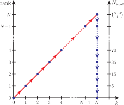
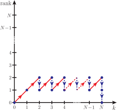
Figure 6: Evolution of the tensor rank R𝑅R and the number Ntcoeff(R)=(R+44)subscript𝑁tcoeff𝑅binomial𝑅44N_{\mathrm{tcoeff}}\,(R)=\binom{R+4}{4} of open-loop tensor coefficients (right vertical axis) as a function of the number k𝑘k of dressed segments during the open-loop recursion. Each dressing step is assumed to increase the rank by one. The original open-loop algorithm, where tensor reduction is applied a posteriori (left), is compared to the on-the-fly reduction approach (right). The red diagonal lines illustrate the dressing steps and the blue vertical lines the reduction steps.

As demonstrated in Section 6.2, performing helicity sums and merging diagrams on-the-fly yields a very significant efficiency improvement with respect to the original open-loop algorithm. More precisely, if helicity sums are performed at the end of the recursion as in (53), the merging approach and the parent–child relations (46) permit to achieve a similar speed-up factor of the order of two. However, contrary to the parent–child technique, the on-the-the-fly approach is applicable both to diagram merging and helicity sums. This leads to a further speed-up factor that can vary from two to three, depending on the process.

As we will see in Section 4, the on-the-fly approach will be a crucial ingredient in order to arrive at a new efficient algorithm that combines the operations of open-loop dressing and tensor reduction at the level of each individual step of the open-loop recursion.

4 On-the-fly reduction of open loops

In the original version of the OpenLoops program, the construction of integrand numerators and the reduction to scalar integrals are performed independently of one another using different tools. Open-loop numerators of N𝑁N-point diagrams are constructed by recursively dressing N𝑁N segments as described in Section 2.3. Each step of the recursion can increase the tensor rank by one, and, upon symmetrisation of all qμ1qμrsuperscript𝑞subscript𝜇1superscript𝑞subscript𝜇𝑟q^{\mu_{1}}\ldots q^{\mu_{r}} monomials with rR𝑟𝑅r\leq R, open-loop polynomials of rank R𝑅R involve (R+44)binomial𝑅44\binom{R+4}{4} independent tensor coefficients. Thus their complexity grows exponentially with the number of recursion steps. For instance, open loops with R=6𝑅6R=6 and R=7𝑅7R=7 involve, respectively, 210210210 and 330330330 components, while only 555 components are present for R=1𝑅1R=1. As illustrated in the left plot of Fig. 6, in the original open-loop algorithm tensorial complexity keeps growing until the maximum rank RN𝑅𝑁R\leq N is reached at the end of the dressing recursion. At this stage, upon summation of helicity configurations and loop diagrams with equivalent one-loop topology, tensor integrals are reduced to scalar integrals using external libraries, such as Collier Denner:2014gla or Cuttools Ossola:2007ax , as described in Section 2.5.

Dealing with intermediate results with a large number of tensor components requires a considerable amount of computing power, both for the reduction of high-rank objects and at the level of the tensorial structure of the open-loop recursion (42), which needs to be performed for each relevant helicity configuration and each []β0βksuperscriptsubscriptdelimited-[]subscript𝛽0subscript𝛽𝑘[\dots]_{\beta_{0}}^{\beta_{k}} component. These operations can be significantly accelerated by means of the techniques introduced in Section 3. Nevertheless, they remain the most CPU intensive aspect of multi-particle one-loop calculations in OpenLoops.

Motivated by the above considerations, in this section we introduce a new approach that avoids the appearance of high-rank objects at any stage of the calculation. This is achieved by extending the on-the-fly approach introduced in Section 3 to the reduction of open loops. In this way, interleaving the operations of open-loop dressing and tensor reduction, we build a single recursive algorithm, where each increase of tensorial rank caused by a dressing step is compensated by an integrand-reduction step.

Refer to caption             𝒱2(ΩN2)subscript𝒱2superscriptsubscriptΩ𝑁2\mathcal{V}_{2}(\Omega_{N}^{2}) =\displaystyle= Refer to caption          𝒱2(ΩN2[1])subscript𝒱2superscriptsubscriptΩ𝑁2delimited-[]1\mathcal{V}_{2}\big{(}{\Omega_{N}^{2}[-1]}\big{)}
+ Refer to caption          V2(ΩN2[1]) Refer to caption          V2(ΩN2[1]) \displaystyle+\;\;\raisebox{-2.84526pt}{\parbox[t]{186.6503pt}{\includegraphics[height=52.80846pt]{newdiaredpinchA}\\ \mbox{\hskip 28.45274pt$\mathcal{V}_{2}\big{(}{\Omega_{N}^{2}[1]}\big{)}$}}} +\displaystyle+ Refer to caption          𝒱2(ΩN2[2])subscript𝒱2superscriptsubscriptΩ𝑁2delimited-[]2\mathcal{V}_{2}\big{(}{\Omega_{N}^{2}[2]}\big{)}
+ Refer to caption          V2(ΩN2[3]) Refer to caption          V2(ΩN2[3]) \displaystyle+\;\;\raisebox{-2.84526pt}{\parbox[t]{186.6503pt}{\includegraphics[height=52.80846pt]{newdiaredpinchC}\\ \mbox{\hskip 28.45274pt$\mathcal{V}_{2}\big{(}{\Omega_{N}^{2}[3]}\big{)}$}}} +\displaystyle+ Refer to caption          𝒱2(ΩN2[0])subscript𝒱2superscriptsubscriptΩ𝑁2delimited-[]0\mathcal{V}_{2}\big{(}{\Omega_{N}^{2}[0]}\big{)}
Figure 7: Diagrammatic representation of the on-the-fly reduction step (79) for an N𝑁N-point open loop at step k=2𝑘2k=2 of the dressing recursion. The symbols 𝒱k(ΩNk)subscript𝒱𝑘subscriptsuperscriptΩ𝑘𝑁\mathcal{V}_{k}(\Omega^{k}_{N}) and 𝒱k(ΩNk[j])subscript𝒱𝑘subscriptsuperscriptΩ𝑘𝑁delimited-[]𝑗\mathcal{V}_{k}(\Omega^{k}_{N}[j]) correspond, respectively, to the rank-two polynomial on the lhs of (79) and its reduced rank-one counterparts on the rhs. The red crosses indicate the pinching of the D¯jsubscript¯𝐷𝑗\bar{D}_{j} propagators in the 𝒱k(ΩNk[j])subscript𝒱𝑘subscriptsuperscriptΩ𝑘𝑁delimited-[]𝑗\mathcal{V}_{k}(\Omega^{k}_{N}[j]) terms with j=0,,3𝑗03j=0,\dots,3. Since D¯0=D¯Nsubscript¯𝐷0subscript¯𝐷𝑁\bar{D}_{0}=\bar{D}_{N}, in our graphical representation the D¯0subscript¯𝐷0\bar{D}_{0} denominator is located on the Nthsuperscript𝑁thN^{\mathrm{th}} segment.

As illustrated in the right plot of Fig. 6, the on-the-fly reduction approach avoids the appearance of any intermediate object with rank higher than two. Besides the CPU cost needed for the processing of high-rank objects, this alleviates also possible memory issues due to their storage.

4.1 On-the-fly integrand reduction

For the on-the-fly reduction of open-loop polynomials we are going to use the method of delAguila:2004nf , which permits to reduce rank-two monomials of the loop momentum through identities of the form

qμqνsuperscript𝑞𝜇superscript𝑞𝜈\displaystyle q^{\mu}q^{\nu} =\displaystyle= [A1μν+A0μνD0]+[B1,λμν+j=03Bj,λμνDj]qλ.delimited-[]subscriptsuperscript𝐴𝜇𝜈1subscriptsuperscript𝐴𝜇𝜈0subscript𝐷0delimited-[]subscriptsuperscript𝐵𝜇𝜈1𝜆superscriptsubscript𝑗03subscriptsuperscript𝐵𝜇𝜈𝑗𝜆subscript𝐷𝑗superscript𝑞𝜆\displaystyle\left[A^{\mu\nu}_{-1}+A^{\mu\nu}_{0}D_{0}\right]+\left[B^{\mu\nu}_{-1,\lambda}+\sum\limits_{j=0}^{3}B^{\mu\nu}_{j,\lambda}D_{j}\right]q^{\lambda}{}.

The rank-one polynomial on the rhs is a linear combination of four loop denominators, D0,,D3subscript𝐷0subscript𝐷3D_{0},\dots,D_{3}, and the corresponding tensor coefficients, Ajμνsuperscriptsubscript𝐴𝑗𝜇𝜈A_{j}^{\mu\nu} and Bj,λμνsuperscriptsubscript𝐵𝑗𝜆𝜇𝜈B_{j,\lambda}^{\mu\nu}, depend only on the three external momenta p1,p2,p3subscript𝑝1subscript𝑝2subscript𝑝3p_{1},p_{2},p_{3}. The coefficients of loop denominators are labeled with indices j=0,,3𝑗03j=0,\dots,3, while j=1𝑗1j=-1 is used for the constant parts. Their explicit expressions are presented in Section 5.2.

The identity (LABEL:eq:qmuqnuredfinal) provides an exact reconstruction of qμqνsuperscript𝑞𝜇superscript𝑞𝜈q^{\mu}q^{\nu} in terms of four-dimensional loop denominators, but can be easily generalised to D𝐷D-dimensional denominators by replacing

DjD¯jq~2forj=0,1,2,3.formulae-sequencesubscript𝐷𝑗subscript¯𝐷𝑗superscript~𝑞2for𝑗0123\displaystyle D_{j}\to\bar{D}_{j}-\tilde{q}^{2}\quad\mbox{for}\quad j=0,1,2,3\,. (78)

Note that q~2superscript~𝑞2\tilde{q}^{2} contributions resulting from the terms Bj,λμνDjsubscriptsuperscript𝐵𝜇𝜈𝑗𝜆subscript𝐷𝑗B^{\mu\nu}_{j,\lambda}D_{j} with j=0,1,2,3𝑗0123j=0,1,2,3 must cancel among each other in (LABEL:eq:qmuqnuredfinal) since they generate rank-three terms of type qλq~2superscript𝑞𝜆superscript~𝑞2q^{\lambda}\,\tilde{q}^{2} that are not consistent with the rank-two structure on the lhs. Thus the substitutions (78) generate only an extra term q~2A0μνsuperscript~𝑞2superscriptsubscript𝐴0𝜇𝜈-\tilde{q}^{2}A_{0}^{\mu\nu} on the rhs of (LABEL:eq:qmuqnuredfinal).

The integrand reduction (LABEL:eq:qmuqnuredfinal) holds at the integrand level, irrespectively of the presence of extra loop denominators D4,,DN1subscript𝐷4subscript𝐷𝑁1D_{4},\dots,D_{N-1} or additional q𝑞q-dependent factors that may multiply the qμqνsuperscript𝑞𝜇superscript𝑞𝜈q^{\mu}q^{\nu} monomial. These properties, in combination with the factorisation of open loops into segments, make it possible to apply the reduction (LABEL:eq:qmuqnuredfinal) at any intermediate stage of the recursion (73). This on-the-fly reduction approach is illustrated in Fig. 7, and the corresponding reduction identities for N𝑁N-point integrands at step k𝑘k of the dressing recursion have the form

𝒱k(ΩNk,q¯)Sk+1(q)SN(q)D¯0D¯3D¯N1=subscript𝒱𝑘subscriptsuperscriptΩ𝑘𝑁¯𝑞subscript𝑆𝑘1𝑞subscript𝑆𝑁𝑞subscript¯𝐷0subscript¯𝐷3subscript¯𝐷𝑁1absent\displaystyle\frac{\mathcal{V}_{k}(\Omega^{k}_{N},\bar{q})\;S_{k+1}(q)\cdots S_{N}(q)}{\bar{D}_{0}\cdots\bar{D}_{3}\cdots\bar{D}_{N-1}}=
=j=13𝒱k(ΩNk[j],q¯)Sk+1(q)SN(q)D¯0D¯jD¯3D¯N1,absentsuperscriptsubscript𝑗13subscript𝒱𝑘subscriptsuperscriptΩ𝑘𝑁delimited-[]𝑗¯𝑞subscript𝑆𝑘1𝑞subscript𝑆𝑁𝑞subscript¯𝐷0subscript¯𝐷𝑗subscript¯𝐷3subscript¯𝐷𝑁1\displaystyle=\sum_{j=-1}^{3}\frac{\mathcal{V}_{k}(\Omega^{k}_{N}[j],\bar{q})\;S_{k+1}(q)\cdots S_{N}(q)}{\bar{D}_{0}\cdots\not{\bar{D}_{j}}\cdots\bar{D}_{3}\cdots\bar{D}_{N-1}}, (79)

where ΩNk[j]subscriptsuperscriptΩ𝑘𝑁delimited-[]𝑗\Omega^{k}_{N}[j] for 0j30𝑗30\leq j\leq 3 denote the (N1)𝑁1(N-1)-point subtopologies that arise from ΩNksubscriptsuperscriptΩ𝑘𝑁\Omega^{k}_{N} by pinching the D¯jsubscript¯𝐷𝑗\bar{D}_{j} propagator, while terms with j=1𝑗1j=-1 on the rhs correspond to the original topology, ΩNk[1]=ΩNksubscriptsuperscriptΩ𝑘𝑁delimited-[]1subscriptsuperscriptΩ𝑘𝑁\Omega^{k}_{N}[-1]=\Omega^{k}_{N}. Note that the denominators D¯jsubscript¯𝐷𝑗\bar{D}_{j} can be pinched irrespectively of whether the related Sj(q)subscript𝑆𝑗𝑞S_{j}(q) segments are already dressed or not. In (79) we adopt the approach of Section 3.2, where open-loop polynomials incorporate the colour-summed interference with the Born amplitude as well as helicity sums and merging of all dressed segments. However, for simplicity, the bookkeeping of helicities, merged diagrams, and []β0βksuperscriptsubscriptdelimited-[]subscript𝛽0subscript𝛽𝑘[\dots]_{\beta_{0}}^{\beta_{k}} indices is kept implicit.

The partially dressed open loops on the lhs and rhs of (79) have the general form

𝒱k(Ω,q¯)=s=0Sr=0R𝒱k;μ1μrs(Ω)qμ1qμrq~2s,subscript𝒱𝑘Ω¯𝑞superscriptsubscript𝑠0𝑆superscriptsubscript𝑟0𝑅subscriptsuperscript𝒱𝑠𝑘subscript𝜇1subscript𝜇𝑟Ωsuperscript𝑞subscript𝜇1superscript𝑞subscript𝜇𝑟superscript~𝑞2𝑠\displaystyle\mathcal{V}_{k}(\Omega,\bar{q})=\sum_{s=0}^{S}\sum_{r=0}^{R}\mathcal{V}^{s}_{k;\mu_{1}\dots\mu_{r}}(\Omega)\,q^{\mu_{1}}\cdots q^{\mu_{r}}\,\tilde{q}^{2s},\quad (80)

where four-dimensional loop-momentum components are accompanied by q~2superscript~𝑞2\tilde{q}^{2} terms that arise from (LABEL:eq:qmuqnuredfinal)-(78). As discussed in Section 4.4, only a small fraction of the q~2superscript~𝑞2\tilde{q}^{2}-dependent terms can lead to non-vanishing contributions at the end of the recursion. Thus, in order to avoid the proliferation of tensor coefficients, all q~2superscript~𝑞2\tilde{q}^{2} terms that are expected to vanish are identified and discarded in advance at each dressing and reduction step.

In general, the relation (79) allows one to reduce any polynomial 𝒱k(ΩNk,q¯)subscript𝒱𝑘subscriptsuperscriptΩ𝑘𝑁¯𝑞\mathcal{V}_{k}(\Omega^{k}_{N},\bar{q}) of rank R2𝑅2R\geq 2 to rank R1𝑅1R-1 polynomials 𝒱k(ΩNk[j],q¯)subscript𝒱𝑘subscriptsuperscriptΩ𝑘𝑁delimited-[]𝑗¯𝑞\mathcal{V}_{k}(\Omega^{k}_{N}[j],\bar{q}). But, in practice, the reduction (79) can be interleaved with the open-loop dressing recursion in a way that the tensor rank never exceeds two. For R=2𝑅2R=2 the coefficients of the rank-one open-loop polynomials that arise from the reduction (79) read

𝒱k;s(ΩNk[j])subscriptsuperscript𝒱𝑠𝑘subscriptsuperscriptΩ𝑘𝑁delimited-[]𝑗\displaystyle\mathcal{V}^{s}_{k;}(\Omega^{k}_{N}[j]) =\displaystyle= 𝒱k;ν1ν2s(ΩNk)Ajν1ν2+δ1j[𝒱k;s(ΩNk)\displaystyle\mathcal{V}^{s}_{k;\nu_{1}\nu_{2}}(\Omega^{k}_{N})A_{j}^{\nu_{1}\nu_{2}}+\delta_{-1j}\left[\mathcal{V}^{s}_{k;}(\Omega^{k}_{N})\right.
𝒱k;ν1ν2s1(ΩNk)A0ν1ν2],\displaystyle-\left.\mathcal{V}^{s-1}_{k;\nu_{1}\nu_{2}}(\Omega^{k}_{N})A_{0}^{\nu_{1}\nu_{2}}\right],
𝒱k;μ1s(ΩNk[j])subscriptsuperscript𝒱𝑠𝑘subscript𝜇1subscriptsuperscriptΩ𝑘𝑁delimited-[]𝑗\displaystyle\mathcal{V}^{s}_{k;\mu_{1}}(\Omega^{k}_{N}[j]) =\displaystyle= 𝒱k;ν1ν2s(ΩNk)Bj,μ1ν1ν2+δ1j𝒱k;μ1s(ΩNk).subscriptsuperscript𝒱𝑠𝑘subscript𝜈1subscript𝜈2subscriptsuperscriptΩ𝑘𝑁superscriptsubscript𝐵𝑗subscript𝜇1subscript𝜈1subscript𝜈2subscript𝛿1𝑗subscriptsuperscript𝒱𝑠𝑘subscript𝜇1subscriptsuperscriptΩ𝑘𝑁\displaystyle\mathcal{V}^{s}_{k;\nu_{1}\nu_{2}}(\Omega^{k}_{N})B_{j,\mu_{1}}^{\nu_{1}\nu_{2}}+\delta_{-1j}\mathcal{V}^{s}_{k;\mu_{1}}(\Omega^{k}_{N}).

The transformations (79)(LABEL:eq:OFRmasterformulaB) can be used to reduce any rank-two open loop with N4𝑁4N\geq 4 propagators to a rank-one N𝑁N-point object and four (N1)𝑁1(N-1)-point pinched objects of rank one.

Rank-two open loops with only N=3𝑁3N=3 loop propagators can be reduced to rank one in a very similar way delAguila:2004nf . The relevant identities (see Section 5.3) have the same structure as (LABEL:eq:qmuqnuredfinal) but involve only three reconstructed propagators, D¯0subscript¯𝐷0\bar{D}_{0}, D¯1subscript¯𝐷1\bar{D}_{1} and D¯2subscript¯𝐷2\bar{D}_{2}. Moreover, they do not hold at the integrand level, but only upon integration over the loop momentum. The tensors Ajμνsuperscriptsubscript𝐴𝑗𝜇𝜈A_{j}^{\mu\nu} and Bj,λμνsuperscriptsubscript𝐵𝑗𝜆𝜇𝜈B_{j,\lambda}^{\mu\nu} for the case N=3𝑁3N=3 depend only on p1subscript𝑝1p_{1} and p2subscript𝑝2p_{2}. They are obtained from the ones for N=4𝑁4N=4 by simply setting to zero the terms involving p3subscript𝑝3p_{3} (see Section 5.3).

The on-the-fly reduction formula for N=3𝑁3N=3 has the form

dDq¯𝒱k(Ω3k,q¯)Srem(q)D¯0D¯2=superscriptd𝐷¯𝑞subscript𝒱𝑘subscriptsuperscriptΩ𝑘3¯𝑞subscript𝑆rem𝑞subscript¯𝐷0subscript¯𝐷2absent\displaystyle\int\!\mathrm{d}^{D}\!\bar{q}\,\frac{\mathcal{V}_{k}(\Omega^{k}_{3},\bar{q})\;S_{\mathrm{rem}}(q)}{\bar{D}_{0}\cdots\bar{D}_{2}}=
=j=12dDq¯𝒱k(Ω3k[j],q¯)Srem(q)D¯0D¯jD¯2,absentsuperscriptsubscript𝑗12superscriptd𝐷¯𝑞subscript𝒱𝑘subscriptsuperscriptΩ𝑘3delimited-[]𝑗¯𝑞subscript𝑆rem𝑞subscript¯𝐷0subscript¯𝐷𝑗subscript¯𝐷2\displaystyle=\sum_{j=-1}^{2}\int\!\mathrm{d}^{D}\!\bar{q}\,\frac{\mathcal{V}_{k}(\Omega^{k}_{3}[j],\bar{q})\;S_{\mathrm{rem}}(q)}{\bar{D}_{0}\cdots\not{\bar{D}_{j}}\cdots\bar{D}_{2}}, (82)

where 𝒱k(Ω3k,q¯)subscript𝒱𝑘subscriptsuperscriptΩ𝑘3¯𝑞\mathcal{V}_{k}(\Omega^{k}_{3},\bar{q}) is an open loop of rank R=2𝑅2R=2 that results from a certain number k2𝑘2k\geq 2 of dressing steps and k2𝑘2k-2 or less reduction steps. Possible undressed segments are denoted as Srem(q)subscript𝑆rem𝑞S_{\mathrm{rem}}(q), and (82) is valid only for terms Srem(q)subscript𝑆rem𝑞S_{\mathrm{rem}}(q) of rank zero or one. In general this allows for only Nrem1subscript𝑁rem1N_{\mathrm{rem}}\leq 1 extra segments, i.e.

Srem(q)={Sk+1(q)forNrem=1 1forNrem=0,subscript𝑆rem𝑞casessubscript𝑆𝑘1𝑞forsubscript𝑁rem11forsubscript𝑁rem0\displaystyle S_{\mathrm{rem}}(q)=\begin{cases}\;S_{k+1}(q)&\mbox{for}\;N_{\mathrm{rem}}=1\\[5.69054pt] \;1&\mbox{for}\;N_{\mathrm{rem}}=0\end{cases}\;\;, (83)

and these two cases are sufficient to cover all relevant N=3𝑁3N=3 topologies and pinched subtopologies in renormalisable theories.333The fact that Nrem1subscript𝑁rem1N_{\mathrm{rem}}\leq 1 follows from the inequality Nrem+RNunpinched0,subscript𝑁rem𝑅subscript𝑁unpinched0N_{\mathrm{rem}}+R-N_{\mathrm{unpinched}}\leq 0, where R=2𝑅2R=2 is the rank of 𝒱k(Ω3k,q¯)subscript𝒱𝑘subscriptsuperscriptΩ𝑘3¯𝑞\mathcal{V}_{k}(\Omega^{k}_{3},\bar{q}), and Nunpinched=3subscript𝑁unpinched3N_{\mathrm{unpinched}}=3 is the number of unpinched propagators in (82). The above inequality is obviously fulfilled at the beginning of the open-loop recursion, where k=R=NremNunpinched=0𝑘𝑅subscript𝑁remsubscript𝑁unpinched0k=R=N_{\mathrm{rem}}-N_{\mathrm{unpinched}}=0, and its validity is guaranteed by the fact that, in renormalisable theories, dressing and reduction steps cannot increase Nrem+RNunpinchedsubscript𝑁rem𝑅subscript𝑁unpinchedN_{\mathrm{rem}}+R-N_{\mathrm{unpinched}}. The relations between the rank-two polynomial 𝒱k(Ω3k,q¯)subscript𝒱𝑘subscriptsuperscriptΩ𝑘3¯𝑞\mathcal{V}_{k}(\Omega^{k}_{3},\bar{q}) and its reduced counterparts 𝒱k(Ω3k[j],q¯)subscript𝒱𝑘subscriptsuperscriptΩ𝑘3delimited-[]𝑗¯𝑞\mathcal{V}_{k}(\Omega^{k}_{3}[j],\bar{q}) have the same form as in (LABEL:eq:OFRmasterformulaB).

Although the above three-point reduction holds only at the integral level, the fact that the term Srem(q)subscript𝑆rem𝑞S_{\mathrm{rem}}(q) can be factorised makes it possible to apply (82) as soon as the dressed open loop 𝒱k(Ω3k,q¯)subscript𝒱𝑘subscriptsuperscriptΩ𝑘3¯𝑞\mathcal{V}_{k}(\Omega^{k}_{3},\bar{q}) has reached rank two, independently of the remaining part of the numerator.

In summary, exploiting the fact that open loops are factorised into segments, the identities (LABEL:eq:qmuqnuredfinal) and (82) can be applied on-the-fly during the dressing recursion, while an arbitrary number of segments is still undressed.444Note that the fact that the technique of delAguila:2004nf can be applied on-the-fly is not a general feature of integrand reduction methods. For instance, the OPP method Ossola:2006us is not applicable on-the-fly since it is based on the multiple poles of the entire integrand. Thus, dressing and reduction steps can be interleaved in a way that the increase of tensorial rank resulting from dressing is promptly compensated through an on-the-fly reduction. More precisely, on-the-fly reduction steps are applied to diagrams and pinched sub-diagrams with N3𝑁3N\geq 3 at those stages of the recursion where the next dressing step would generate a rank-three object.555This means that, before performing an on-the-fly reduction, rank-two open loops are first dressed with all possible adjacent segments of rank zero. Delaying the reduction step in this way reduces the additional CPU cost that results from the appearance of new pinched objects. The reduced rank-one objects with N𝑁N and N1𝑁1N-1 loop propagators are further dressed and possibly reduced until one arrives at fully dressed open loops of rank R2𝑅2R\leq 2 for all two- and higher-point contributions. An this stage, the open-loop matrix structure can be eliminated by taking the trace (76), and all rank-two objects with N3𝑁3N\geq 3 can be reduced to rank one with a final reduction step of type (LABEL:eq:qmuqnuredfinal) or (82).

After the above dressing and on-the-fly reduction steps, the following types of integrals remain to be reduced:

  • (i)

    integrals with N5𝑁5N\geq 5 loop propagators
    and rank R=1,0𝑅10R=1,0;

  • (ii)

    integrals with N=4,3𝑁43N=4,3 loop propagators
    and rank R=1𝑅1R=1; \tagform@84

  • (iii)

    integrals with N=2𝑁2N=2 loop propagators
    and rank R=2,1𝑅21R=2,1.

For their reduction to scalar integrals with N4𝑁4N\leq 4 we use a combination of integral reduction and OPP reduction identities as described in A.

4.2 Merging pinched topologies

Since it allows one to keep the tensor rank low at any stage of the calculations, the on-the-fly reduction approach has the potential to accelerate one-loop calculations in a significant way. However, some aspects of the on-the-fly reduction approach could lead to a dramatic increase of the computational cost. First, the fact that the reduction is performed when the loop is still open, i.e. before taking the trace (76), implies that the entries of the []β0βksuperscriptsubscriptdelimited-[]subscript𝛽0subscript𝛽𝑘[\dots]_{\beta_{0}}^{\beta_{k}} matrix have to be processed as 16 independent objects. Second, the reduction has to be performed for all not yet summed helicity configurations of the undressed segments. Third, each reduction step (79) generates four pinched topologies that need to be processed as independent contributions in subsequent dressing and reduction steps.

Due to the proliferation of pinched subtopologies, the naive iteration of on-the-fly reduction steps would lead to a dramatic increase of the CPU cost. Fortunately, this can be avoided by means of the merging technique introduced in Section 3.2, which makes it possible to absorb pinched N𝑁N-point open loops into unpinched (N1)𝑁1(N-1)-point open loops, in such a way that they do not need to be processed as separate objects. As explained in the following, the merging of pinched subtopologies requires a different implementation depending on whether the pinch belongs to the dressed part of the open loop or not, as well as for the special case of a D¯0subscript¯𝐷0\bar{D}_{0} pinch.

Refer to caption=αj,αj+1Refer to captionRefer to captionsubscriptsubscript𝛼𝑗subscript𝛼𝑗1Refer to caption\displaystyle\raisebox{-14.22636pt}{\parbox[t]{143.40157pt}{\includegraphics[height=59.18185pt]{newdiaredpinchG}}}\quad=\quad{\sum_{\scriptstyle{\alpha_{j},\alpha_{j+1}}}}\;\raisebox{-14.22636pt}{\parbox[t]{159.33539pt}{\includegraphics[height=59.18185pt]{newdiaredpinchI}}}
+αj,αj+1Refer to caption+Refer to captionsubscriptsubscript𝛼𝑗subscript𝛼𝑗1Refer to captionRefer to caption\displaystyle+{\sum_{\scriptstyle{\alpha_{j},\alpha_{j+1}}}}\;\raisebox{-14.22636pt}{\parbox[t]{159.33539pt}{\includegraphics[height=59.18185pt]{newdiaredpinchIb}}}\quad+\quad\raisebox{-14.22636pt}{\parbox[t]{168.44012pt}{\includegraphics[height=59.18185pt]{newdiaredpinchF}}}
Figure 8: Diagrammatic representation of formula (90) for the merging of pinched open loops. The first two unpinched diagrams on the rhs, where the generic subtrees wjαjsuperscriptsubscript𝑤𝑗subscript𝛼𝑗w_{j}^{\alpha_{j}} and wj+1αj+1superscriptsubscript𝑤𝑗1subscript𝛼𝑗1w_{j+1}^{\alpha_{j+1}} are directly connected to the loop propagators D~j1subscript~𝐷𝑗1\widetilde{D}_{j-1} and D~jsubscript~𝐷𝑗\widetilde{D}_{j}, correspond to the first term on the rhs of (90). The corresponding triple or quartic vertices of the Feynman rules play an analogous role as the crossed vertex in the pinched open loop (last diagram on the rhs). Besides merging all relevant unpinched combinations αj,αj+1subscript𝛼𝑗subscript𝛼𝑗1\alpha_{j},\alpha_{j+1}, also possible unpinched topologies where some of the external legs in wjsubscript𝑤𝑗w_{j} and wj+1subscript𝑤𝑗1w_{j+1} are interchanged (not shown) should be included.

4.2.1 Pinching a dressed propagator

Let us consider the on-the-fly reduction of an N𝑁N-point open loop with k𝑘k dressed segments, focusing on contributions that result from the pinching of a D¯jsubscript¯𝐷𝑗\bar{D}_{j} denominator with j<k𝑗𝑘j<k,

[Uncaptioned image]=[Uncaptioned image]absent\displaystyle\raisebox{-14.22636pt}{\parbox[t]{191.20233pt}{\includegraphics[height=59.18185pt]{newdiaredpinchE}}}=
=𝒱kαk+1αN(ΩNk[j],q¯)Sk+1αk+1(q)SNαN(q)D¯0D¯jD¯3D¯N1.absentsubscriptsuperscript𝒱subscript𝛼𝑘1subscript𝛼𝑁𝑘subscriptsuperscriptΩ𝑘𝑁delimited-[]𝑗¯𝑞superscriptsubscript𝑆𝑘1subscript𝛼𝑘1𝑞superscriptsubscript𝑆𝑁subscript𝛼𝑁𝑞subscript¯𝐷0subscript¯𝐷𝑗subscript¯𝐷3subscript¯𝐷𝑁1\displaystyle=\frac{\mathcal{V}^{\alpha_{k+1}\dots\alpha_{N}}_{k}(\Omega^{k}_{N}[j],\bar{q})\;S_{k+1}^{\alpha_{k+1}}(q)\cdots S_{N}^{\alpha_{N}}(q)}{\bar{D}_{0}\cdots\not{\bar{D}_{j}}\cdots\bar{D}_{3}\cdots\bar{D}_{N-1}}.\qquad (85)

Here, consistently with the notation of Section 3.2, we have restored the indices αisubscript𝛼𝑖\alpha_{i} of the various undressed segments, while helicity indices are kept implicit. The pinched propagator in (4.2.1) is entirely dressed and merged, in the sense that both adjacent segments, Sjsubscript𝑆𝑗S_{j} and Sj+1subscript𝑆𝑗1S_{j+1}, are dressed and merged. Thus, for what concerns all future dressing and reduction steps, apart from the disappearance of the D¯jsubscript¯𝐷𝑗\bar{D}_{j} denominator, the pinch has no effect. Consequently, the above contribution can be absorbed into unpinched (N1)𝑁1(N-1)-point open loops that involve the same loop denominators, D¯0D¯j1D¯j+1D¯N1subscript¯𝐷0subscript¯𝐷𝑗1subscript¯𝐷𝑗1subscript¯𝐷𝑁1\bar{D}_{0}\dots\bar{D}_{j-1}\bar{D}_{j+1}\dots\bar{D}_{N-1}, and the same undressed segments, Sk+1αk+1,,SN1αN1superscriptsubscript𝑆𝑘1subscript𝛼𝑘1superscriptsubscript𝑆𝑁1subscript𝛼𝑁1S_{k+1}^{\alpha_{k+1}},\dots,S_{N-1}^{\alpha_{N-1}}. To this end, it is sufficient to bring the pinched open loop (4.2.1) in the standard form

[Uncaptioned image]=[Uncaptioned image]absent\displaystyle\;\raisebox{-14.22636pt}{\parbox[t]{154.78267pt}{\includegraphics[height=59.18185pt]{newdiaredpinchF}}}=
=[Uncaptioned image],absent[Uncaptioned image]\displaystyle=\;\raisebox{-14.22636pt}{\parbox[t]{191.20233pt}{\includegraphics[height=59.18185pt]{newdiaredpinchE}}}\;,\qquad (86)

which corresponds to an unpinched (N1)𝑁1(N-1)-point open loop with k1𝑘1k-1 dressed segments. The crossed vertex on the lhs of (4.2.1) indicates that the two original segments that are connected by the pinched propagator should be regarded as a single effective segment. This symbolic contraction of segments does not change anything in the numerics of the open-loop numerator, and the transformation (4.2.1) is nothing but a trivial relabeling of the denominators and of the undressed segments that lie on the right side of the pinch,

D~i(q)=D¯i(q)fori<j,D~i(q)=D¯i+1(q)andS~iαi(q)=Si+1αi+1(q)forij.subscript~𝐷𝑖𝑞subscript¯𝐷𝑖𝑞missing-subexpressionmissing-subexpressionmissing-subexpressionmissing-subexpressionfor𝑖𝑗subscript~𝐷𝑖𝑞subscript¯𝐷𝑖1𝑞andsubscriptsuperscript~𝑆subscript𝛼𝑖𝑖𝑞superscriptsubscript𝑆𝑖1subscript𝛼𝑖1𝑞for𝑖𝑗\displaystyle\begin{array}[]{rclcrclcc}\widetilde{D}_{i}(q)&=&\bar{D}_{i}(q)&&&&&\;\mbox{for}&i<j,\\[11.38109pt] \widetilde{D}_{i}(q)&=&\bar{D}_{i+1}(q)&\,\text{and}&\widetilde{S}^{\alpha_{i}}_{i}(q)&=&S_{i+1}^{\alpha_{i+1}}(q)&\;\mbox{for}&i\geq j.\\[2.84526pt] \end{array} (89)

The pinched open loop (4.2.1) can be merged with corresponding unpinched open loops to form a single (N1)𝑁1(N-1)-point object with k1𝑘1k-1 dressed segments. The corresponding formula reads

𝒱~k1αkαN1(Ω~N1k1,q¯)S~kαk(q)S~N1αN1(q)D~0D~3D~N2=subscriptsuperscript~𝒱subscript𝛼𝑘subscript𝛼𝑁1𝑘1subscriptsuperscript~Ω𝑘1𝑁1¯𝑞subscriptsuperscript~𝑆subscript𝛼𝑘𝑘𝑞superscriptsubscript~𝑆𝑁1subscript𝛼𝑁1𝑞subscript~𝐷0subscript~𝐷3subscript~𝐷𝑁2absent\displaystyle\frac{\widetilde{\mathcal{V}}^{\alpha_{k}\dots\alpha_{N-1}}_{k-1}(\widetilde{\Omega}^{k-1}_{N-1},\bar{q})\;\widetilde{S}^{\alpha_{k}}_{k}(q)\cdots\widetilde{S}_{N-1}^{\alpha_{N-1}}(q)}{\widetilde{D}_{0}\cdots\widetilde{D}_{3}\cdots\widetilde{D}_{N-2}}=
=𝒱k1αkαN1(ΩN1k1,q¯)S~kαk(q)S~N1αN1(q)D~0D~3D~N2absentsubscriptsuperscript𝒱subscript𝛼𝑘subscript𝛼𝑁1𝑘1superscriptsubscriptΩ𝑁1𝑘1¯𝑞subscriptsuperscript~𝑆subscript𝛼𝑘𝑘𝑞superscriptsubscript~𝑆𝑁1subscript𝛼𝑁1𝑞subscript~𝐷0subscript~𝐷3subscript~𝐷𝑁2\displaystyle=\frac{\mathcal{V}^{\alpha_{k}\dots\alpha_{N-1}}_{k-1}(\Omega_{N-1}^{k-1},\bar{q})\;\widetilde{S}^{\alpha_{k}}_{k}(q)\cdots\widetilde{S}_{N-1}^{\alpha_{N-1}}(q)}{\widetilde{D}_{0}\cdots\widetilde{D}_{3}\cdots\widetilde{D}_{N-2}}
+ΩNk[j]𝒱~kαkαN1(ΩNk[j],q¯)Sk+1αk(q)SNαN1(q)D¯0D¯jD¯3D¯N1.subscriptsubscriptsuperscriptΩ𝑘𝑁delimited-[]𝑗superscriptsubscript~𝒱𝑘subscript𝛼𝑘subscript𝛼𝑁1subscriptsuperscriptΩ𝑘𝑁delimited-[]𝑗¯𝑞superscriptsubscript𝑆𝑘1subscript𝛼𝑘𝑞superscriptsubscript𝑆𝑁subscript𝛼𝑁1𝑞subscript¯𝐷0subscript¯𝐷𝑗subscript¯𝐷3subscript¯𝐷𝑁1\displaystyle+\!\sum_{\Omega^{k}_{N}[j]}\!\frac{\widetilde{\mathcal{V}}_{k}^{\alpha_{k}\dots\alpha_{N-1}}(\Omega^{k}_{N}[j],\bar{q})\;S_{k+1}^{\alpha_{k}}(q)\cdots S_{N}^{\alpha_{N-1}}(q)}{\bar{D}_{0}\cdots\not{\bar{D}_{j}}\cdots\bar{D}_{3}\cdots\bar{D}_{N-1}}.\qquad (90)

A diagrammatic representation of this identity is given in Fig. 8. The resulting object, for which we introduce the symbol 𝒱~k1αkαN1subscriptsuperscript~𝒱subscript𝛼𝑘subscript𝛼𝑁1𝑘1\widetilde{\mathcal{V}}^{\alpha_{k}\dots\alpha_{N-1}}_{k-1}, is a combination of unpinched and pinched open loops, which enter, respectively, through the first and second term on the rhs of (90). By construction, the corresponding set of diagrams (Ω~N1k1superscriptsubscript~Ω𝑁1𝑘1\widetilde{\Omega}_{N-1}^{k-1}) includes all unpinched (ΩN1k1superscriptsubscriptΩ𝑁1𝑘1\Omega_{N-1}^{k-1}) and pinched (ΩNk[j]subscriptsuperscriptΩ𝑘𝑁delimited-[]𝑗\Omega^{k}_{N}[j]) diagrams with loop propagators D~0D~N2subscript~𝐷0subscript~𝐷𝑁2\widetilde{D}_{0}\dots\widetilde{D}_{N-2} and undressed segments Sk+1αk+1,,SN1αN1superscriptsubscript𝑆𝑘1subscript𝛼𝑘1superscriptsubscript𝑆𝑁1subscript𝛼𝑁1S_{k+1}^{\alpha_{k+1}},\dots,S_{N-1}^{\alpha_{N-1}}. The set of pinched diagrams ΩNk[j]subscriptsuperscriptΩ𝑘𝑁delimited-[]𝑗\Omega^{k}_{N}[j] corresponds to an N𝑁N-point topology that results from Ωk1N1superscriptsubscriptΩ𝑘1𝑁1\Omega_{k-1}^{N-1} by undoing a D¯jsubscript¯𝐷𝑗\bar{D}_{j} pinch, and (90) involves all possible ΩNk[j]subscriptsuperscriptΩ𝑘𝑁delimited-[]𝑗\Omega^{k}_{N}[j] contributions with 1jk1𝑗𝑘1\leq j\leq k.

As a necessary condition for the merging operation (90) to be applicable, the different open loops on the rhs of (90) have to feature the same undressed segments. This implies that they must be at the same stage of the dressing recursion, and, most importantly, that the starting position and the directions of the respective dressing recursions should be equivalent to each other. With other words, D~0D~N2subscript~𝐷0subscript~𝐷𝑁2\widetilde{D}_{0}\dots\widetilde{D}_{N-2} and D¯0D¯jD¯N1subscript¯𝐷0subscript¯𝐷𝑗subscript¯𝐷𝑁1\bar{D}_{0}\dots\not{\bar{D}_{j}}\dots\bar{D}_{N-1} should be two identical ordered sets of propagators. In particular they should start from the same cut propagator, D~0=D¯0subscript~𝐷0subscript¯𝐷0\widetilde{D}_{0}=\bar{D}_{0}. As discussed in Section 4.3 this can be guaranteed, to some extent, by means of an appropriate cutting rule.

Another obvious prerequisite for the absorption of pinched N𝑁N-point open loops is the existence of corresponding unpinched (N1)𝑁1(N-1)-point Feynman diagrams. With other words, the crossed vertex in (4.2.1) should have a physical counterpart consisting of a triple or quartic vertex, which can directly connect the D¯j1subscript¯𝐷𝑗1\bar{D}_{j-1} and D¯j+1subscript¯𝐷𝑗1\bar{D}_{j+1} propagators to subtrees involving the external legs attached to w^jsubscript^𝑤𝑗\hat{w}_{j} and w^j+1subscript^𝑤𝑗1\hat{w}_{j+1} (see Fig. 8). In QCD, this turns out to be the case for most pinched configurations.

Moreover, pinched N𝑁N-point configurations of the form (4.2.1) can also be merged with other pinched higher-point diagrams that get the relevant pinches in past or future reduction steps. Thus, pinched objects of type (4.2.1) will always be denoted as absorbable, irrespective of whether corresponding unpinched (N1)𝑁1(N-1)-point Feynman diagrams exist or not.

The merging procedure (90) needs to be applied after any on-the-fly reduction step that creates new pinched objects. Thus merging operations have to be interleaved with iterated dressing and reduction steps. Since pinched N𝑁N-point objects are absorbed into lower-point objects, the algorithm should start with the dressing and on-the-fly reduction of open loops with N=Nmax𝑁subscript𝑁N=N_{\max}, and continue towards lower N𝑁N. The merging operation (90) starts at stage N1=Nmax1𝑁1subscript𝑁1N-1=N_{\max}-1 and is applied after every dressing step, together with the merging of unpinched open loops (see Section 3.2). Note that, due to the iterative nature of the algorithm, the term 𝒱~kαkαN1subscriptsuperscript~𝒱subscript𝛼𝑘subscript𝛼𝑁1𝑘\widetilde{\mathcal{V}}^{\alpha_{k}\dots\alpha_{N-1}}_{k} on the rhs of (90) can be the result of multiple pinching and merging steps.

=\displaystyle= αk+1,,αj+1Refer to captionsubscriptsubscript𝛼𝑘1subscript𝛼𝑗1Refer to caption\displaystyle\sum_{\alpha_{k+1},\dots,\alpha_{j+1}}\raisebox{-14.22636pt}{\parbox[t]{191.20233pt}{ \includegraphics[height=59.18185pt]{newdiaredpinchL}}}
Refer to caption
Figure 9: Required dressing (4.2.2) and relabeling (89) operations before merging open loops with an undressed pinched propagator D¯jsubscript¯𝐷𝑗\bar{D}_{j}.

4.2.2 Pinching an undressed propagator

The possibility to absorb pinched open loops as in Fig. 8 is based on the fact that all future dressing and reduction operations can be performed only once at the level of a merged object. Thus, the undressed segments of pinched and unpinched open loops should be identical.

However, the segments connected to the D~j1subscript~𝐷𝑗1\widetilde{D}_{j-1} and D~jsubscript~𝐷𝑗\widetilde{D}_{j} propagators are different for pinched and unpinched terms. In the pinched case there are two separate segments, which involve wjsubscript𝑤𝑗w_{j} and wj+1subscript𝑤𝑗1w_{j+1} and require two subsequent dressing steps. In contrast, unpinched open loops require a single dressing step, since wjsubscript𝑤𝑗w_{j} and wj+1subscript𝑤𝑗1w_{j+1} are combined in a single segment.

It is thus clear that pinched open loops can be absorbed only after the dressing of the segments that lie on the two sides of the pinch. If this is not the case, i.e. when a D¯jsubscript¯𝐷𝑗\bar{D}_{j} pinch is applied to an open loop with kj𝑘𝑗k\leq j dressed segments, its absorption becomes possible only after (kj+1)𝑘𝑗1(k-j+1) additional dressing steps, which result in

𝒱~j+1αj+1αN1(ΩNj+1[j],q¯)=superscriptsubscript~𝒱𝑗1subscript𝛼𝑗1subscript𝛼𝑁1subscriptsuperscriptΩ𝑗1𝑁delimited-[]𝑗¯𝑞absent\displaystyle\widetilde{\mathcal{V}}_{j+1}^{\alpha_{j+1}\dots\alpha_{N-1}}(\Omega^{j+1}_{N}[j],\bar{q})=
=αk+1αj+1𝒱~kαk+1αj+1αj+1αN1(ΩNk[j],q¯)absentsubscriptsubscriptsuperscript𝛼𝑘1subscriptsuperscript𝛼𝑗1superscriptsubscript~𝒱𝑘subscriptsuperscript𝛼𝑘1subscriptsuperscript𝛼𝑗1subscript𝛼𝑗1subscript𝛼𝑁1subscriptsuperscriptΩ𝑘𝑁delimited-[]𝑗¯𝑞\displaystyle=\sum_{\alpha^{\prime}_{k+1}\dots\alpha^{\prime}_{j+1}}\widetilde{\mathcal{V}}_{k}^{\alpha^{\prime}_{k+1}\dots\alpha^{\prime}_{j+1}\alpha_{j+1}\dots\alpha_{N-1}}(\Omega^{k}_{N}[j],\bar{q})
×Sk+1αk+1(q)Sj+1αj+1(q),absentsuperscriptsubscript𝑆𝑘1subscriptsuperscript𝛼𝑘1𝑞superscriptsubscript𝑆𝑗1subscriptsuperscript𝛼𝑗1𝑞\displaystyle\phantom{=\sum_{\alpha^{\prime}_{k+1}\dots\alpha^{\prime}_{j+1}}}\times\,S_{k+1}^{\alpha^{\prime}_{k+1}}(q)\cdots S_{j+1}^{\alpha^{\prime}_{j+1}}(q), (91)

where Sk+1Sj+1subscript𝑆𝑘1subscript𝑆𝑗1S_{k+1}\dots S_{j+1} are dressed. Note that in (4.2.2) we also sum over all possible αisubscriptsuperscript𝛼𝑖\alpha^{\prime}_{i}, and use indices αj+1,,αN1subscript𝛼𝑗1subscript𝛼𝑁1\alpha_{j+1},\dots,\alpha_{N-1} with shifted labels for the undressed segments Sj+2,,SNsubscript𝑆𝑗2subscript𝑆𝑁S_{j+2},\dots,S_{N} on the right side of the pinch.

As illustrated in Fig. 9, the dressing operation (4.2.2) combined with the relabeling (89) brings the pinched open loops in a configuration that can be absorbed with the merging formula (90). However, the absorption of undressed pinched propagators is more involved than the simplified picture of Fig. 9. Pinched open loops can require more than one dressing step to become absorbable, in which case, in general, also new reduction steps are needed in order to keep the tensor rank below three. Such new reductions generate additional pinches, and their iteration can lead to a proliferation of multi-pinched configurations.

Thus, to avoid dramatic inefficiencies, it is crucial to minimise the number of required dressing steps by keeping pinchable propagators as close as possible to the dressed part of the numerator. This is why we choose to perform the on-the-fly reduction using the denominators D¯0,,D¯3subscript¯𝐷0subscript¯𝐷3\bar{D}_{0},\dots,\bar{D}_{3}.666The on-the-fly reduction (79) can be performed using any set of four propagators, D¯i0,,D¯i3subscript¯𝐷subscript𝑖0subscript¯𝐷subscript𝑖3\bar{D}_{i_{0}},\ldots,\bar{D}_{i_{3}}. In this way, when the first two segments are dressed and the first reduction step is applied (see Fig. 7), the various pinched propagators are located at most one left-dressing step (D¯0subscript¯𝐷0\bar{D}_{0}) and two right-dressing steps (D¯3subscript¯𝐷3\bar{D}_{3}) away from the dressed part.

In order to identify pinches that cannot be directly absorbed and to anticipate how they propagate through the recursion, let us consider generic open-loop configurations before the creation of a new pinch through a reduction step. At this stage the rank R𝑅R must be equal to two. We first consider the very first reduction step, which can occur after kR=2𝑘𝑅2k\geq R=2 dressing steps, and we focus on a D¯2subscript¯𝐷2\bar{D}_{2} pinch in the case where only k=2𝑘2k=2 segments are dressed. In this case, an on-the-fly reduction step and a subsequent dressing step yield

(92)
¯D2-pinch +dressing [Uncaptioned image]FRACOP ¯D2-pinch +dressing [Uncaptioned image]\displaystyle{\longrightarrow\atop\mbox{\parbox{42.67912pt}{$\bar{D}_{2}$-pinch\\ +dressing}}}\raisebox{-11.38109pt}{\parbox[t]{145.67793pt}{\includegraphics[height=59.18185pt]{flowdiaredpinchX}}}

i.e. the D¯2subscript¯𝐷2\bar{D}_{2} pinch can be brought in the standard form (4.2.1) and can thus be absorbed into unpinched contributions. The same considerations apply also to D¯1subscript¯𝐷1\bar{D}_{1} and D¯0subscript¯𝐷0\bar{D}_{0} pinches (see Section 4.2.3) and can be generalised to any step of the recursion, since the structure of the dressed parts on the lhs and rhs of (92) is the same.

Also D¯3subscript¯𝐷3\bar{D}_{3} pinches can be absorbed in a similar way in case there are at least three dressed segments before the reduction step. Otherwise, when only two segments are dressed, the combination of an on-the-fly reduction step with a subsequent dressing step leads to

(93)
¯D3-pinch +dressing [Uncaptioned image]FRACOP ¯D3-pinch +dressing [Uncaptioned image]\displaystyle{\longrightarrow\atop\mbox{\parbox{42.67912pt}{$\bar{D}_{3}$-pinch\\ +dressing}}}\raisebox{-11.38109pt}{\parbox[t]{177.54488pt}{\includegraphics[height=59.18185pt]{flowdiaredpinchC}}}

where the pinch is applied on the last dressed segment. Unless another dressing step can be applied before reaching rank three, this kind of pinch cannot be absorbed without a further reduction and dressing step. Dressing one more segment allows one to absorb the original D3subscript𝐷3D_{3} pinch as well as new D¯0subscript¯𝐷0\bar{D}_{0}, D¯1subscript¯𝐷1\bar{D}_{1}, and D¯2subscript¯𝐷2\bar{D}_{2} pinches that arise from the new reduction step. However, the new reduction leads again to a configuration with a D~3subscript~𝐷3\widetilde{D}_{3} pinch on the last dressed segment,

(94)
~D3-pinch +dressing [Uncaptioned image]FRACOP ~D3-pinch +dressing [Uncaptioned image]\displaystyle{\longrightarrow\atop\mbox{\parbox{42.67912pt}{$\widetilde{D}_{3}$-pinch\\ +dressing}}}\raisebox{-11.38109pt}{\parbox[t]{177.54488pt}{\includegraphics[height=59.18185pt]{flowdiaredpinchY}}}

Again, the dressed parts on the lhs and rhs of (94) have the same structure, which implies that such D¯3subscript¯𝐷3\bar{D}_{3}-pinched configurations are stable with respect to further reduction steps. Thus, open loops with multiple non-absorbable pinches do not occur, and the only type of configuration with a single non-absorbable pinch is the one in (94).

=\displaystyle= αNRefer to captionsubscriptsubscript𝛼𝑁Refer to caption\displaystyle{\sum_{\alpha_{N}}}\hskip 5.69054pt\raisebox{-14.22636pt}{\parbox[t]{191.20233pt}{\includegraphics[height=59.18185pt]{newdiaredpinchO}}}
Refer to caption
Figure 10: Required dressing, loop-momentum shift and relabeling operations  (96)(101) before merging an open loop with a pinched D¯0subscript¯𝐷0\bar{D}_{0} propagator.

4.2.3 Pinching the D¯0subscript¯𝐷0\bar{D}_{0} propagator

Finally, we consider open loops with k𝑘k dressed segments and a pinched D¯0subscript¯𝐷0\bar{D}_{0} denominator,

[Uncaptioned image]=[Uncaptioned image]absent\displaystyle\raisebox{-14.22636pt}{\parbox[t]{191.20233pt}{\includegraphics[height=59.18185pt]{newdiaredpinchNb}}}=
=𝒱kαk+1αN(ΩNk[0],q¯)Sk+1αk+1(q)SNαN(q)D¯1D¯3D¯N1D¯0.absentsubscriptsuperscript𝒱subscript𝛼𝑘1subscript𝛼𝑁𝑘subscriptsuperscriptΩ𝑘𝑁delimited-[]0¯𝑞superscriptsubscript𝑆𝑘1subscript𝛼𝑘1𝑞superscriptsubscript𝑆𝑁subscript𝛼𝑁𝑞subscript¯𝐷1subscript¯𝐷3subscript¯𝐷𝑁1subscript¯𝐷0\displaystyle=\frac{\mathcal{V}^{\alpha_{k+1}\dots\alpha_{N}}_{k}(\Omega^{k}_{N}[0],\bar{q})\;S_{k+1}^{\alpha_{k+1}}(q)\cdots S_{N}^{\alpha_{N}}(q)}{\bar{D}_{1}\cdots\bar{D}_{3}\cdots\bar{D}_{N-1}\not{\bar{D}_{0}}}.\qquad (95)

For convenience, here and in the following we put D¯0subscript¯𝐷0\bar{D}_{0} at the end of the chain of denominators. Similarly as for the cases discussed in Section 4.2.2, the above pinched configuration becomes absorbable only when the segments connected to the D¯0subscript¯𝐷0\bar{D}_{0} propagator, i.e. SN(q)subscript𝑆𝑁𝑞S_{N}(q) and S1(q)subscript𝑆1𝑞S_{1}(q), are dressed. However, this happens only at the end of the standard dressing recursion.

In order to anticipate the absorption of the most advanced pinch one could replace the denominators D¯0,,D¯3subscript¯𝐷0subscript¯𝐷3\bar{D}_{0},\dots,\bar{D}_{3} used for the on-the-fly reduction by D¯1,,D¯4subscript¯𝐷1subscript¯𝐷4\bar{D}_{1},\dots,\bar{D}_{4}, which lie all directly on the right side of the cut. However, the absorption of each D¯4subscript¯𝐷4\bar{D}_{4} pinch would require up to three extra dressing steps and two related reduction steps, resulting in the creation of multiple new pinches. This problem can be circumvented by observing that the D¯0subscript¯𝐷0\bar{D}_{0} propagator lies only one step away from the dressed part of the open loop, if one reverts the dressing direction. Therefore, as illustrated in Fig. 10, the pinched D¯0subscript¯𝐷0\bar{D}_{0} propagator can be entirely dressed by means of a single left-dressing step. This operation results in

𝒱~k+1αk+1αN1(ΩNk+1[0],q¯)=superscriptsubscript~𝒱𝑘1subscript𝛼𝑘1subscript𝛼𝑁1subscriptsuperscriptΩ𝑘1𝑁delimited-[]0¯𝑞absent\displaystyle\widetilde{\mathcal{V}}_{k+1}^{\alpha_{k+1}\dots\alpha_{N-1}}(\Omega^{k+1}_{N}[0],\bar{q})=
=αNSNαN(q)𝒱~kαk+1αN1αN(ΩNk[0],q¯),absentsubscriptsubscript𝛼𝑁superscriptsubscript𝑆𝑁subscript𝛼𝑁𝑞superscriptsubscript~𝒱𝑘subscript𝛼𝑘1subscript𝛼𝑁1subscript𝛼𝑁subscriptsuperscriptΩ𝑘𝑁delimited-[]0¯𝑞\displaystyle=\sum_{\alpha_{N}}S_{N}^{\alpha_{N}}(q)\;\widetilde{\mathcal{V}}_{k}^{\alpha_{k+1}\dots\alpha_{N-1}\alpha_{N}}(\Omega^{k}_{N}[0],\bar{q}), (96)

where the left multiplication of the Nthsuperscript𝑁thN^{\mathrm{th}} segment should be understood as

[SN(q)𝒱~k(Ω,q¯)]β0βk+1=βN[SN(q)]β0βNsubscriptsuperscriptdelimited-[]subscript𝑆𝑁𝑞subscript~𝒱𝑘Ω¯𝑞subscript𝛽𝑘1subscript𝛽0subscriptsubscript𝛽𝑁subscriptsuperscriptdelimited-[]subscript𝑆𝑁𝑞subscript𝛽𝑁subscript𝛽0\displaystyle\Big{[}S_{N}(q)\;\widetilde{\mathcal{V}}_{k}(\Omega,\bar{q})\Big{]}^{\beta_{k+1}}_{\beta_{0}}=\sum_{\beta_{N}}\Big{[}S_{N}(q)\Big{]}^{\beta_{N}}_{\beta_{0}}
×[𝒱~k(Ω,q¯)]βNβk+1=[([𝒱~k(Ω,q¯)]T[SN(q)]T)T]β0βk+1.\displaystyle\times\,\Big{[}\widetilde{\mathcal{V}}_{k}(\Omega,\bar{q})\!\Big{]}^{\beta_{k+1}}_{\beta_{N}}=\left[\left(\Big{[}\widetilde{\mathcal{V}}_{k}(\Omega,\bar{q})\Big{]}^{\mathrm{T}}\;\Big{[}S_{N}(q)\Big{]}^{\mathrm{T}}\right)^{\mathrm{T}}\;\right]^{\beta_{k+1}}_{\beta_{0}}.
(97)

Technically, as indicated on the rhs, this operation can be easily implemented through a standard right-dressing step upon transposition of the input matrices and back-transposition of the result.777Note that in a three-gluon vertex this transposition leads to a flip of the colour indices of the two gluons in the loop and hence a minus sign in the colour factor. Since the colour factor has been fixed in the beginning this minus sign has to be taken into account in the colour-stripped open loop.

As usual, before merging with unpinched open loops, the propagators and undressed segments that lie on the right side of the pinch need to be brought back in standard form. In case of a D¯0subscript¯𝐷0\bar{D}_{0} pinch, all remaining N1𝑁1N-1 denominators and segments preserve their relative position along the open loop. Thus, only D¯N1subscript¯𝐷𝑁1\bar{D}_{N-1} needs to be relabeled, since it assumes the role of the new D~0subscript~𝐷0\widetilde{D}_{0}. Moreover, the standard form D~0=q2m~02subscript~𝐷0superscript𝑞2subscriptsuperscript~𝑚20\widetilde{D}_{0}=q^{2}-\widetilde{m}^{2}_{0} requires a loop momentum shift qqpN1𝑞𝑞subscript𝑝𝑁1q\to q-p_{N-1} for the entire open loop. The corresponding reparametrisations for the various denominators and segments read

D~0(q)=D¯N1(qpN1),D~i(q)=D¯i(qpN1)for1iN2,S~iαi(q)=Siαi(qpN1)fork+1iN1.subscript~𝐷0𝑞subscript¯𝐷𝑁1𝑞subscript𝑝𝑁1missing-subexpressionmissing-subexpressionsubscript~𝐷𝑖𝑞subscript¯𝐷𝑖𝑞subscript𝑝𝑁1for1𝑖𝑁2subscriptsuperscript~𝑆subscript𝛼𝑖𝑖𝑞superscriptsubscript𝑆𝑖subscript𝛼𝑖𝑞subscript𝑝𝑁1for𝑘1𝑖𝑁1\displaystyle\begin{array}[]{rclcl}\widetilde{D}_{0}(q)&=&\bar{D}_{N-1}(q-p_{N-1}),&&\\[8.53581pt] \widetilde{D}_{i}(q)&=&\bar{D}_{i}(q-p_{N-1})&\;\mbox{for}&1\leq i\leq N-2,\\[8.53581pt] \widetilde{S}^{\alpha_{i}}_{i}(q)&=&S_{i}^{\alpha_{i}}(q-p_{N-1})&\;\mbox{for}&k+1\leq i\leq N-1.\end{array} (101)

In terms of masses and momenta this corresponds to m~0=mN1subscript~𝑚0subscript𝑚𝑁1\widetilde{m}_{0}=m_{N-1}, m~i=misubscript~𝑚𝑖subscript𝑚𝑖\widetilde{m}_{i}=m_{i} and p~i=pi+pN1subscript~𝑝𝑖subscript𝑝𝑖subscript𝑝𝑁1\widetilde{p}_{i}=p_{i}+p_{N-1} for 1iN21𝑖𝑁21\leq i\leq N-2. With these transformations the left-dressed D¯0subscript¯𝐷0\bar{D}_{0}-pinched open loop (96) can be merged with related unpinched objects according to

𝒱~kαk+1αN1(Ω~N1k,q¯)S~k+1αk+1(q)S~N1αN1(q)D¯1D~3D~N2D~0subscriptsuperscript~𝒱subscript𝛼𝑘1subscript𝛼𝑁1𝑘subscriptsuperscript~Ω𝑘𝑁1¯𝑞subscriptsuperscript~𝑆subscript𝛼𝑘1𝑘1𝑞superscriptsubscript~𝑆𝑁1subscript𝛼𝑁1𝑞subscript¯𝐷1subscript~𝐷3subscript~𝐷𝑁2subscript~𝐷0absent\displaystyle\frac{\widetilde{\mathcal{V}}^{\alpha_{k+1}\dots\alpha_{N-1}}_{k}(\widetilde{\Omega}^{k}_{N-1},\bar{q})\widetilde{S}^{\alpha_{k+1}}_{k+1}(q)\cdots\widetilde{S}_{N-1}^{\alpha_{N-1}}(q)}{\bar{D}_{1}\cdots\widetilde{D}_{3}\cdots\widetilde{D}_{N-2}\widetilde{D}_{0}}\equiv
𝒱kαk+1αN1(ΩN1k,q¯)S~k+1αk+1(q)S~N1αN1(q)D¯1D~3D~N2D~0absentsubscriptsuperscript𝒱subscript𝛼𝑘1subscript𝛼𝑁1𝑘superscriptsubscriptΩ𝑁1𝑘¯𝑞subscriptsuperscript~𝑆subscript𝛼𝑘1𝑘1𝑞superscriptsubscript~𝑆𝑁1subscript𝛼𝑁1𝑞subscript¯𝐷1subscript~𝐷3subscript~𝐷𝑁2subscript~𝐷0\displaystyle\equiv\;\frac{\mathcal{V}^{\alpha_{k+1}\dots\alpha_{N-1}}_{k}(\Omega_{N-1}^{k},\bar{q})\widetilde{S}^{\alpha_{k+1}}_{k+1}(q)\cdots\widetilde{S}_{N-1}^{\alpha_{N-1}}(q)}{\bar{D}_{1}\cdots\widetilde{D}_{3}\cdots\widetilde{D}_{N-2}\widetilde{D}_{0}}
+ΩNk[0]𝒱~k+1αk+1αN1(ΩNk+1[0],q¯)D¯1D¯3D¯N1D¯0subscriptsubscriptsuperscriptΩ𝑘𝑁delimited-[]0superscriptsubscript~𝒱𝑘1subscript𝛼𝑘1subscript𝛼𝑁1subscriptsuperscriptΩ𝑘1𝑁delimited-[]0¯𝑞subscript¯𝐷1subscript¯𝐷3subscript¯𝐷𝑁1subscript¯𝐷0\displaystyle\phantom{\equiv}+\sum_{\Omega^{k}_{N}[0]}\frac{\widetilde{\mathcal{V}}_{k+1}^{\alpha_{k+1}\dots\alpha_{N-1}}(\Omega^{k+1}_{N}[0],\bar{q})}{\bar{D}_{1}\cdots\bar{D}_{3}\cdots\bar{D}_{N-1}\not{\bar{D}_{0}}}
×Sk+1αk+1(q)SN1αN1(q)|qqpN1.absentevaluated-atsuperscriptsubscript𝑆𝑘1subscript𝛼𝑘1𝑞superscriptsubscript𝑆𝑁1subscript𝛼𝑁1𝑞𝑞𝑞subscript𝑝𝑁1\displaystyle\phantom{\equiv}\times\,S_{k+1}^{\alpha_{k+1}}(q)\cdots S_{N-1}^{\alpha_{N-1}}(q)\Bigg{|}_{q\to q-p_{N-1}}. (102)

Apart from the loop momentum shift, qqpN1𝑞𝑞subscript𝑝𝑁1q\to q-p_{N-1}, this formula is entirely analogous to (90). Let us note that, since the shift is applied to a single term, the identity (102) holds only upon loop momentum integration. Nevertheless, as far as the correctness of final results at integral level is concerned, it can be safely applied at the integrand level.

As demonstrated in Section 6.2, using the on-the fly reduction with pinch absorption in combination with the on-the-fly techniques of Section 3 results in a very fast and numerically stable one-loop algorithm. In particular, as compared to the original version of OpenLoops, we find very significant improvements, both in terms of speed and numerical stability. Actually, using only the new techniques of Section 3 without on-the-fly reduction yields even higher CPU efficiency. However, as we will see, the moderate extra CPU cost that results from the on-the-fly reduction approach is counterbalanced by a very significant gain in numerical stability, which implies a reduced usage of quadruple precision for exceptional phase space points.

4.3 Cutting rule

As pointed out in Section 4.2.1, the possibility to merge pinched N𝑁N-point open loops and corresponding unpinched (N1)𝑁1(N-1)-point open loops depends on the way they are cut. In order to identify the relevant requirements, let us consider the cut-open topology defined by the following ordered set of loop segments,

N={𝒮1,𝒮2,,𝒮N}.subscript𝑁subscript𝒮1subscript𝒮2subscript𝒮𝑁\displaystyle\mathcal{I}_{N}=\{\mathcal{S}_{1},\mathcal{S}_{2},\dots,\mathcal{S}_{N}\}. (103)

Here we have applied our standard labeling scheme, where the cut is located between 𝒮Nsubscript𝒮𝑁\mathcal{S}_{N} and 𝒮1subscript𝒮1\mathcal{S}_{1}, i.e. on the D¯0subscript¯𝐷0\bar{D}_{0} propagator, while the dressing recursion starts with 𝒮1subscript𝒮1\mathcal{S}_{1} and is directed towards 𝒮2subscript𝒮2\mathcal{S}_{2}. This configuration will be referred to as a 𝒮Nsubscript𝒮𝑁\mathcal{S}_{N}/𝒮1subscript𝒮1\mathcal{S}_{1} ordered cut. Since the labeling scheme is a consequence of the position of the cut, and not vice versa, we have to define a cutting rule that selects 𝒮Nsubscript𝒮𝑁\mathcal{S}_{N}/𝒮1subscript𝒮1\mathcal{S}_{1} out of all possible 𝒮isubscript𝒮𝑖\mathcal{S}_{i}/𝒮jsubscript𝒮𝑗\mathcal{S}_{j} cuts.

The cutting rule should enable the merging of pinched subtopologies that arise from (103) by pinching certain propagators D¯jsubscript¯𝐷𝑗\bar{D}_{j}, i.e. by combining 𝒮jsubscript𝒮𝑗\mathcal{S}_{j} and 𝒮j+1subscript𝒮𝑗1\mathcal{S}_{j+1} in a single segment 𝒮j𝒮j+1direct-sumsubscript𝒮𝑗subscript𝒮𝑗1\mathcal{S}_{j}\oplus\mathcal{S}_{j+1}. To this end, unless the cut propagator D¯0subscript¯𝐷0\bar{D}_{0} is pinched, the cutting rule should guarantee that the position of the cut and its direction remain unchanged after a pinch. More explicitly, the desired cut configurations after a D¯jsubscript¯𝐷𝑗\bar{D}_{j} pinch with j>0𝑗0j>0 are

N[1]subscript𝑁delimited-[]1\displaystyle\mathcal{I}_{N}[1] =\displaystyle= {𝒮1𝒮2,𝒮3,,𝒮N},direct-sumsubscript𝒮1subscript𝒮2subscript𝒮3subscript𝒮𝑁\displaystyle\{\mathcal{S}_{1}\oplus\mathcal{S}_{2},\mathcal{S}_{3},\dots,\mathcal{S}_{N}\}, (104)
N[j]subscript𝑁delimited-[]𝑗\displaystyle\mathcal{I}_{N}[j] =\displaystyle= {𝒮1,,𝒮j1,𝒮j𝒮j+1,𝒮j+2,,𝒮N}subscript𝒮1subscript𝒮𝑗1direct-sumsubscript𝒮𝑗subscript𝒮𝑗1subscript𝒮𝑗2subscript𝒮𝑁\displaystyle\{\mathcal{S}_{1},\dots,\mathcal{S}_{j-1},\mathcal{S}_{j}\oplus\mathcal{S}_{j+1},\mathcal{S}_{j+2},\dots,\mathcal{S}_{N}\} (105)
for 2jN2,for2𝑗𝑁2\displaystyle\mbox{for}\;2\leq j\leq N-2,
N[N1]subscript𝑁delimited-[]𝑁1\displaystyle\mathcal{I}_{N}[N-1] =\displaystyle= {𝒮1,𝒮2,,𝒮N1𝒮N}.subscript𝒮1subscript𝒮2direct-sumsubscript𝒮𝑁1subscript𝒮𝑁\displaystyle\{\mathcal{S}_{1},\mathcal{S}_{2},\dots,\mathcal{S}_{N-1}\oplus\mathcal{S}_{N}\}. (106)

In this way, as required for the merging operations described in Sections 4.2.14.2.2, the dressing of pinched and unpinched objects always starts and ends with segments that contain the external legs attached to 𝒮1subscript𝒮1\mathcal{S}_{1} and 𝒮Nsubscript𝒮𝑁\mathcal{S}_{N}, respectively. In the case of a D¯0subscript¯𝐷0\bar{D}_{0} pinch, where the original cut propagator disappears, in order to enable the merging of left-dressed pinched subtopologies described in Section 4.2.3, the cut should be moved to the left of 𝒮N𝒮1direct-sumsubscript𝒮𝑁subscript𝒮1\mathcal{S}_{N}\oplus\mathcal{S}_{1}, so that

N[0]subscript𝑁delimited-[]0\displaystyle\mathcal{I}_{N}[0] =\displaystyle= {𝒮N𝒮1,𝒮2,,𝒮N1}.direct-sumsubscript𝒮𝑁subscript𝒮1subscript𝒮2subscript𝒮𝑁1\displaystyle\{\mathcal{S}_{N}\oplus\mathcal{S}_{1},\mathcal{S}_{2},\dots,\mathcal{S}_{N-1}\}. (107)

In order to ensure, at least in part, that pinched topologies are cut as in (104)(107), we replace the original cutting rule (49)(50) by the new prescriptions

F(𝒮1)𝐹subscript𝒮1\displaystyle F(\mathcal{S}_{1}) >F(𝒮k)k>1,formulae-sequenceabsent𝐹subscript𝒮𝑘for-all𝑘1\displaystyle>F(\mathcal{S}_{k})\quad\forall\quad k>1,\; (selection rule) (108)
F(𝒮N)𝐹subscript𝒮𝑁\displaystyle F(\mathcal{S}_{N}) >F(𝒮2),absent𝐹subscript𝒮2\displaystyle>F(\mathcal{S}_{2}), (direction rule) (109)

where the weights F(𝒮a)𝐹subscript𝒮𝑎F(\mathcal{S}_{a}) are defined in (47). The key property of the above cutting rule is the pinch-invariance of the selection rule, which determines the first segment 𝒮1subscript𝒮1\mathcal{S}_{1}. In fact, if this condition is realised for (103), then it is guaranteed to hold also for all pinched configurations (104)(107). For j=0,1𝑗01j=0,1 this is an obvious consequence of the fact that F(𝒮1𝒮a)>F(𝒮1)𝐹direct-sumsubscript𝒮1subscript𝒮𝑎𝐹subscript𝒮1F(\mathcal{S}_{1}\oplus\mathcal{S}_{a})>F(\mathcal{S}_{1}) for any a1𝑎1a\neq 1. In the other cases, the fact that 𝒮1subscript𝒮1\mathcal{S}_{1} remains the first subtree in spite of the appearance of a new pinched subtree 𝒮j𝒮j+1direct-sumsubscript𝒮𝑗subscript𝒮𝑗1\mathcal{S}_{j}\oplus\mathcal{S}_{j+1} with weight F(𝒮j)+F(𝒮j+1)𝐹subscript𝒮𝑗𝐹subscript𝒮𝑗1F(\mathcal{S}_{j})+F(\mathcal{S}_{j+1}), is guaranteed by

F(𝒮1)>i=2NF(𝒮i).𝐹subscript𝒮1superscriptsubscript𝑖2𝑁𝐹subscript𝒮𝑖\displaystyle F(\mathcal{S}_{1})>\sum_{i=2}^{N}F(\mathcal{S}_{i}). (110)

This inequality is an automatic consequence of (108) and of the binary nature of the weights (47). This is easily understood by observing that, due to 2Np1=1+α=1Np1 2α1superscript2subscript𝑁p11superscriptsubscript𝛼1subscript𝑁p1superscript2𝛼12^{N_{\mathrm{p}}-1}=1+\sum_{\alpha=1}^{N_{\mathrm{p}}-1}\;2^{\alpha-1}, the last external particle (α=Np𝛼subscript𝑁p\alpha=N_{\mathrm{p}}) outweighs the ensemble of all other particles. Therefore the last external particle must belong to the leading-weight subtree 𝒮1subscript𝒮1\mathcal{S}_{1}, which implies that F(𝒮1)2Np1𝐹subscript𝒮1superscript2subscript𝑁p1F(\mathcal{S}_{1})\geq 2^{N_{\mathrm{p}}-1} and leads to (110).

Unfortunately, the direction rule (109) is not sufficient in order to preserve the direction of the cut. For instance, in case of a D¯1subscript¯𝐷1\bar{D}_{1} pinch, the desired cut (104) requires F(𝒮N)>F(𝒮3)𝐹subscript𝒮𝑁𝐹subscript𝒮3F(\mathcal{S}_{N})>F(\mathcal{S}_{3}), which does not automatically follow from F(𝒮N)>F(𝒮2)𝐹subscript𝒮𝑁𝐹subscript𝒮2F(\mathcal{S}_{N})>F(\mathcal{S}_{2}). More generally, apart from the case of a D3subscript𝐷3D_{3} pinch, where the second and last subtree do not change, there is no guarantee that the condition (109) preserves the direction of the cut.

Thus the above cutting rule does not allow one to absorb all pinched open loops. Nevertheless, as demonstrated in Section 6.2, it is sufficient to obtain a very fast on-the-fly reduction algorithm. Moreover, it should be possible to further increase CPU efficiency, either by means of an improved cutting rule or by inverting the dressing direction after certain pinches.

4.4 Rational terms of type R1subscript𝑅1R_{1}

As discussed in Section 4.1, each reduction step of type (79) and (82) generates terms D¯iDi=q~2subscript¯𝐷𝑖subscript𝐷𝑖superscript~𝑞2\bar{D}_{i}-D_{i}=\tilde{q}^{2} that account for the mismatch between the D𝐷D-dimensional and four-dimensional parts of loop denominators. The resulting tensor integrals with (D4)𝐷4(D-4)-dimensional q~2superscript~𝑞2\tilde{q}^{2} terms in the numerator can give rise to finite terms. As is well known delAguila:2004nf ; Ossola:2008xq , these so-called rational terms of type R1subscript𝑅1R_{1} can arise only in the presence of 1/(D4)1𝐷41/(D-4) poles of ultraviolet type. Thus, vanishing integrals of type R1subscript𝑅1R_{1} can be easily identified by means of the simple power counting criterion

dDq¯qμ1qμ2qμrq~2sD¯0D¯1D¯N1=𝒪(D4)superscriptd𝐷¯𝑞superscript𝑞subscript𝜇1superscript𝑞subscript𝜇2superscript𝑞subscript𝜇𝑟superscript~𝑞2𝑠subscript¯𝐷0subscript¯𝐷1subscript¯𝐷𝑁1𝒪𝐷4\displaystyle\int\!\mathrm{d}^{D}\!\bar{q}\,\frac{q^{\mu_{1}}q^{\mu_{2}}\ldots q^{\mu_{r}}\,\tilde{q}^{2s}}{\bar{D}_{0}\bar{D}_{1}\cdots\bar{D}_{N-1}}=\mathcal{O}(D-4)
ifs1andr+2s+4<2N.formulae-sequenceif𝑠1and𝑟2𝑠42𝑁\displaystyle\qquad\mbox{if}\quad s\geq 1\quad\mbox{and}\quad r+2s+4<2N. (111)

In a renormalisable theory, where each loop segment increases the rank at most by one, r+2sN𝑟2𝑠𝑁r+2s\leq N and all integrals with N5𝑁5N\geq 5 and s1𝑠1s\geq 1 vanish. Thus, the only non-vanishing integrals of type R1subscript𝑅1R_{1} that remain at the end of the on-the-fly reductions of Section 4.1 are delAguila:2004nf

dDq¯q~2D¯0D¯1superscriptd𝐷¯𝑞superscript~𝑞2subscript¯𝐷0subscript¯𝐷1\displaystyle\int\!\mathrm{d}^{D}\!\bar{q}\,\frac{\tilde{q}^{2}}{\bar{D}_{0}\bar{D}_{1}} =\displaystyle= iπ22(m02+m12p123)isuperscript𝜋22superscriptsubscript𝑚02superscriptsubscript𝑚12superscriptsubscript𝑝123\displaystyle\frac{-\mathrm{i}\pi^{2}}{2}\left(m_{0}^{2}+m_{1}^{2}-\frac{p_{1}^{2}}{3}\right) (112)
+𝒪(D4),𝒪𝐷4\displaystyle+\mathcal{O}(D-4),
dDq¯qμq~2D¯0D¯1D¯2superscriptd𝐷¯𝑞superscript𝑞𝜇superscript~𝑞2subscript¯𝐷0subscript¯𝐷1subscript¯𝐷2\displaystyle\int\!\mathrm{d}^{D}\!\bar{q}\,\frac{q^{\mu}\,\tilde{q}^{2}}{\bar{D}_{0}\bar{D}_{1}\bar{D}_{2}} =\displaystyle= iπ26(p1+p2)μisuperscript𝜋26superscriptsubscript𝑝1subscript𝑝2𝜇\displaystyle\frac{\mathrm{i}\pi^{2}}{6}\left(p_{1}+p_{2}\right)^{\mu} (113)
+𝒪(D4),𝒪𝐷4\displaystyle+\mathcal{O}(D-4),
dDq¯q~2D¯0D¯1D¯2superscriptd𝐷¯𝑞superscript~𝑞2subscript¯𝐷0subscript¯𝐷1subscript¯𝐷2\displaystyle\int\!\mathrm{d}^{D}\!\bar{q}\,\frac{\tilde{q}^{2}}{\bar{D}_{0}\bar{D}_{1}\bar{D}_{2}} =\displaystyle= iπ22+𝒪(D4),isuperscript𝜋22𝒪𝐷4\displaystyle\frac{-\mathrm{i}\pi^{2}}{2}+\mathcal{O}(D-4), (114)
dDq¯q~4D¯0D¯1D¯2D¯3superscriptd𝐷¯𝑞superscript~𝑞4subscript¯𝐷0subscript¯𝐷1subscript¯𝐷2subscript¯𝐷3\displaystyle\int\!\mathrm{d}^{D}\!\bar{q}\,\frac{\tilde{q}^{4}}{\bar{D}_{0}\bar{D}_{1}\bar{D}_{2}\bar{D}_{3}} =\displaystyle= iπ26+𝒪(D4).isuperscript𝜋26𝒪𝐷4\displaystyle\frac{-\mathrm{i}\pi^{2}}{6}+\mathcal{O}(D-4). (115)

The power counting criterion (111) can be exploited in a way that makes it possible to discard irrelevant terms of type R1subscript𝑅1R_{1} at any intermediate step of the open-loop recursion. To this end, for each number k𝑘k of dressing steps we anticipate the maximum rank Rkmaxsubscriptsuperscript𝑅𝑘R^{\max}_{k} of the segments Sk+1(q),,SN(q)subscript𝑆𝑘1𝑞subscript𝑆𝑁𝑞S_{k+1}(q),\ldots,S_{N}(q) that remain to be dressed. Given this information, it is clear that monomials of type qμ1qμ2qμrq~2ssuperscript𝑞subscript𝜇1superscript𝑞subscript𝜇2superscript𝑞subscript𝜇𝑟superscript~𝑞2𝑠q^{\mu_{1}}q^{\mu_{2}}\ldots q^{\mu_{r}}\,\tilde{q}^{2s} in the dressed open loop cannot give rise to terms of D𝐷D-dimensional rank higher than r+2s+Rkmax𝑟2𝑠subscriptsuperscript𝑅𝑘r+2s+R^{\max}_{k} at the end of the recursion. Thus, we can anticipate that,

dDq¯qμ1qμrq~2sSk+1(q)SN(q)D¯0D¯1D¯N1=𝒪(D4)superscriptd𝐷¯𝑞superscript𝑞subscript𝜇1superscript𝑞subscript𝜇𝑟superscript~𝑞2𝑠subscript𝑆𝑘1𝑞subscript𝑆𝑁𝑞subscript¯𝐷0subscript¯𝐷1subscript¯𝐷𝑁1𝒪𝐷4\displaystyle\int\!\mathrm{d}^{D}\!\bar{q}\,\frac{q^{\mu_{1}}\ldots q^{\mu_{r}}\,\tilde{q}^{2s}S_{k+1}(q)\dots S_{N}(q)}{\bar{D}_{0}\bar{D}_{1}\cdots\bar{D}_{N-1}}=\mathcal{O}(D-4)
ifs1andr+2s+4+Rkmax<2N.formulae-sequenceif𝑠1and𝑟2𝑠4subscriptsuperscript𝑅𝑘2𝑁\displaystyle\quad\mbox{if}\quad s\geq 1\quad\mbox{and}\quad r+2s+4+R^{\max}_{k}<2N. (116)

The systematic application of this condition allows one to filter out a very large number of q~2superscript~𝑞2\tilde{q}^{2} terms, thereby improving the efficiency of the algorithm.

Note also that the unpinched contributions 𝒱k(ΩNk[1])subscript𝒱𝑘superscriptsubscriptΩ𝑁𝑘delimited-[]1\mathcal{V}_{k}(\Omega_{N}^{k}[-1]) in the reduction identities (LABEL:eq:OFRmasterformulaB) involve terms that reduce r+2s2N𝑟2𝑠2𝑁r+2s-2N, and thus the degree of ultraviolet divergence, by one and two. Depending on the values of N𝑁N and Rkmaxsubscriptsuperscript𝑅𝑘R^{\max}_{k}, this can result in vanishing R1subscript𝑅1R_{1} contributions that can also be immediately discarded. For instance, in the reduction of dDqqμ1qμ2q~2D¯0D¯1D¯2D¯3superscriptd𝐷𝑞superscript𝑞subscript𝜇1superscript𝑞subscript𝜇2superscript~𝑞2subscript¯𝐷0subscript¯𝐷1subscript¯𝐷2subscript¯𝐷3\int\!\mathrm{d}^{D}\!q\,\frac{q^{\mu_{1}}q^{\mu_{2}}\tilde{q}^{2}}{\bar{D}_{0}\bar{D}_{1}\bar{D}_{2}\bar{D}_{3}} all unpinched contributions apart from those of type (115) can be neglected.

5 Reduction identities and numerical stability

This section deals with the reduction method of delAguila:2004nf , which provides the basis of the on-the-fly reduction approach of Section 4.1. In Sections 5.15.3 we outline the derivation of the tensor coefficients Ajμνsuperscriptsubscript𝐴𝑗𝜇𝜈A_{j}^{\mu\nu} and Bj,λμνsubscriptsuperscript𝐵𝜇𝜈𝑗𝜆B^{\mu\nu}_{j,\lambda} in the reduction identities (LABEL:eq:qmuqnuredfinal) and (82). In doing so we set the stage for Section 5.4, where we discuss numerical instability problems and present a systematic approach for their solution.

5.1 The reduction basis

The reduction identities of delAguila:2004nf are based on a decomposition of the four-dimensional loop momentum,

qμ=i=14ciliμ,superscript𝑞𝜇superscriptsubscript𝑖14subscript𝑐𝑖superscriptsubscript𝑙𝑖𝜇\displaystyle q^{\mu}=\sum\limits_{i=1}^{4}c_{i}l_{i}^{\mu}, (117)

in a basis l1,,l4subscript𝑙1subscript𝑙4l_{1},\dots,l_{4}, formed by massless momenta in two orthogonal planes,

li2=0,l1,2l3,4=0.formulae-sequencesuperscriptsubscript𝑙𝑖20subscript𝑙12subscript𝑙340\displaystyle l_{i}^{2}=0,\qquad l_{1,2}\cdot l_{3,4}=0{}. (118)

This reduction basis is defined in terms of the external momenta p1,p2subscript𝑝1subscript𝑝2p_{1},p_{2}, which enter the propagators D1subscript𝐷1D_{1},D2subscript𝐷2D_{2}. The basis momenta l1,2subscript𝑙12l_{1,2} are chosen in the plane spanned by p1subscript𝑝1p_{1} and p2subscript𝑝2p_{2},

l1μ=p1μα1p2μ,l2μ=p2μα2p1μ,formulae-sequencesubscriptsuperscript𝑙𝜇1subscriptsuperscript𝑝𝜇1subscript𝛼1subscriptsuperscript𝑝𝜇2subscriptsuperscript𝑙𝜇2subscriptsuperscript𝑝𝜇2subscript𝛼2subscriptsuperscript𝑝𝜇1\displaystyle l^{\mu}_{1}=p^{\mu}_{1}-\alpha_{1}p^{\mu}_{2},\;\;\;\;\;\;\;l^{\mu}_{2}=p^{\mu}_{2}-\alpha_{2}p^{\mu}_{1}, (119)

while l3,4subscript𝑙34l_{3,4} lie in the plane orthogonal to p1subscript𝑝1p_{1},p2subscript𝑝2p_{2} and are defined as

l3μsubscriptsuperscript𝑙𝜇3\displaystyle l^{\mu}_{3} =\displaystyle= v¯(l1)γμ(1γ52)u(l2),¯𝑣subscript𝑙1superscript𝛾𝜇1superscript𝛾52𝑢subscript𝑙2\displaystyle\bar{v}(l_{1})\gamma^{\mu}\left(\frac{1-\gamma^{5}}{2}\right)u(l_{2}),
l4μsubscriptsuperscript𝑙𝜇4\displaystyle l^{\mu}_{4} =\displaystyle= v¯(l2)γμ(1γ52)u(l1),¯𝑣subscript𝑙2superscript𝛾𝜇1superscript𝛾52𝑢subscript𝑙1\displaystyle\bar{v}(l_{2})\gamma^{\mu}\left(\frac{1-\gamma^{5}}{2}\right)u(l_{1}), (120)

where u𝑢u and v¯¯𝑣\bar{v} are massless spinors. This definition of l3,4subscript𝑙34l_{3,4} implies l3=eiχl4superscriptsubscript𝑙3superscript𝑒i𝜒subscript𝑙4l_{3}^{*}=e^{\mathrm{i}\chi}l_{4}, where χ𝜒\chi is twice the phase difference between the u𝑢u and v𝑣v spinors. The normalization of the basis is chosen such that

γ=2(l1l2)=12(l3l4),𝛾2subscript𝑙1subscript𝑙212subscript𝑙3subscript𝑙4\gamma=2(l_{1}\cdot l_{2})=-\frac{1}{2}(l_{3}\cdot l_{4}){}, (121)

and the α1,2subscript𝛼12\alpha_{1,2} coefficients in (119) read888 The sign of the square root is chosen such that ±Δ=sign(p1p2)Δplus-or-minusΔsignsubscript𝑝1subscript𝑝2Δ\pm\sqrt{\Delta}=\mathrm{sign}(p_{1}\cdot p_{2})\sqrt{\Delta}. This guarantees that the limits limpi20αi=0subscriptsuperscriptsubscript𝑝𝑖20subscript𝛼𝑖0\lim\limits_{p_{i}^{2}\to 0}\alpha_{i}=0 are approached in a smooth way.

αi=pi2(p1p2)±Δ,subscript𝛼𝑖subscriptsuperscript𝑝2𝑖plus-or-minussubscript𝑝1subscript𝑝2Δ\alpha_{i}=\frac{p^{2}_{i}}{(p_{1}\cdot p_{2})\pm\sqrt{\Delta}}, (122)

where ΔΔ\Delta is related to the rank-two Gram determinant Δ12=det(pipj)subscriptΔ12subscript𝑝𝑖subscript𝑝𝑗\Delta_{12}=\det(p_{i}\cdot p_{j}) via

Δ=Δ12=(p1p2)2p12p22.ΔsubscriptΔ12superscriptsubscript𝑝1subscript𝑝22subscriptsuperscript𝑝21subscriptsuperscript𝑝22\Delta=-\Delta_{12}=(p_{1}\cdot p_{2})^{2}-p^{2}_{1}p^{2}_{2}. (123)

The Gram determinant is related to the normalisation factor γ𝛾\gamma via

γ=4Δ(p1p2)±Δ,𝛾4Δplus-or-minussubscript𝑝1subscript𝑝2Δ\gamma=\frac{4\Delta}{(p_{1}\cdot p_{2})\pm\sqrt{\Delta}}, (124)

and these two parameters play a critical role for the stability of the reduction. In fact, in the limit of vanishing Gram determinant, (121) and (124) imply that (l1l2)(l3l4)γΔproportional-tosubscript𝑙1subscript𝑙2subscript𝑙3subscript𝑙4proportional-to𝛾proportional-toΔ(l_{1}\cdot l_{2})\propto(l_{3}\cdot l_{4})\propto\gamma\propto\Delta. Thus

limΔ0(lilj)= 0i,j,subscriptΔ0subscript𝑙𝑖subscript𝑙𝑗 0for-all𝑖𝑗\displaystyle\lim\limits_{\Delta\to 0}\;(l_{i}\cdot l_{j})\;=\;0\qquad\forall\;i,j, (125)

which implies that all light-like basis momenta lisubscript𝑙𝑖l_{i} become parallel to each other999 As a consequence of l1,2μsuperscriptsubscript𝑙12𝜇l_{1,2}^{\mu}\in\mathbb{R} and (l1l2)=E1E2(1cos(θ12))0subscript𝑙1subscript𝑙2subscript𝐸1subscript𝐸21subscript𝜃120(l_{1}\cdot l_{2})=E_{1}E_{2}(1-\cos(\theta_{12}))\to 0, the first two basis vectors become parallel to each other, i.e. l1,2μξ1,2ημsubscriptsuperscript𝑙𝜇12subscript𝜉12superscript𝜂𝜇l^{\mu}_{1,2}\to\xi_{1,2}\,\eta^{\mu} with ξ1,2subscript𝜉12\xi_{1,2}\in\mathbb{R} and ημsuperscript𝜂𝜇\eta^{\mu}\in\mathbb{R}. As for the \mathbb{C}-valued basis vectors l3,4subscript𝑙34l_{3,4}, using l3=eiχl4superscriptsubscript𝑙3superscript𝑒i𝜒subscript𝑙4l_{3}^{*}=e^{\mathrm{i}\chi}{l_{4}} one can define their real and imaginary parts as l3(4),+=[l3(4)+eiχl4(3)]/2subscript𝑙34delimited-[]subscript𝑙34superscript𝑒i𝜒subscript𝑙432l_{3(4),+}=[l_{3(4)}+e^{\mathrm{i}\chi}{l_{4(3)}}]/2, l3(4),=[l3(4)eiχl4(3)]/(2i)subscript𝑙34delimited-[]subscript𝑙34superscript𝑒i𝜒subscript𝑙432il_{3(4),-}=[l_{3(4)}-e^{\mathrm{i}\chi}{l_{4(3)}}]/(2\mathrm{i}), and show that (125) leads to (l~il~j)0subscript~𝑙𝑖subscript~𝑙𝑗0(\tilde{l}_{i}\cdot\tilde{l}_{j})\to 0 for all real-valued vectors l~i,l~j{l1,l2,l3,±,l4,±}subscript~𝑙𝑖subscript~𝑙𝑗subscript𝑙1subscript𝑙2subscript𝑙3plus-or-minussubscript𝑙4plus-or-minus\tilde{l}_{i},\tilde{l}_{j}\in\{l_{1},l_{2},l_{3,\pm},l_{4,\pm}\}. Thus, similarly as for l1,2subscript𝑙12l_{1,2} we have l~iξ~iημisubscript~𝑙𝑖subscript~𝜉𝑖superscript𝜂𝜇for-all𝑖\tilde{l}_{i}\to\tilde{\xi}_{i}\eta^{\mu}\;\forall\;i, and we arrive at l3,4μz3,4ημsubscriptsuperscript𝑙𝜇34subscript𝑧34superscript𝜂𝜇l^{\mu}_{3,4}\to z_{3,4}\eta^{\mu} with z3=z4subscript𝑧3superscriptsubscript𝑧4z_{3}=z_{4}^{*}\in\mathbb{C}, i.e. also the basis vectors l3,4subscript𝑙34l_{3,4} become parallel to l1,2subscript𝑙12l_{1,2}. leading to severe numerical instabilities in the decomposition (117).

Note that in delAguila:2004nf the basis momenta lisubscript𝑙𝑖l_{i} contain an additional normalisation factor101010More explicitly, the basis momenta of delAguila:2004nf correspond to l~i=βlisubscript~𝑙𝑖𝛽subscript𝑙𝑖\tilde{l}_{i}=\beta l_{i} and the various lisubscript𝑙𝑖l_{i}-dependent quantities are related in a similar way, e.g. γ~=β2γ~𝛾superscript𝛽2𝛾\tilde{\gamma}=\beta^{2}\gamma, while lisubscript𝑙𝑖l_{i}-independent quantities such as ΔΔ\Delta and αisubscript𝛼𝑖\alpha_{i} are identical.

β=11α1α2=±(p1p2)±Δ2Δ,𝛽11subscript𝛼1subscript𝛼2plus-or-minusplus-or-minussubscript𝑝1subscript𝑝2Δ2Δ\displaystyle\beta=\frac{1}{1-\alpha_{1}\alpha_{2}}\;=\;\pm\,\frac{(p_{1}\cdot p_{2})\pm\sqrt{\Delta}}{2\sqrt{\Delta}}, (126)

which diverges like 1/Δ1Δ1/\sqrt{\Delta} when Δ0Δ0\Delta\to 0. As a consequence, in delAguila:2004nf numerical instabilities are in part visible as factors β𝛽\beta in the reduction formulas and in part hidden in the definition of the basis vectors. Instead, the basis momenta defined in (119)(120) are stable in the Δ0Δ0\Delta\to 0 limit. Thus, in the reduction formulas presented in Section 5.2 and 5.3, instabilities related to the Gram determinant (123) are fully manifest in the form of inverse powers of the parameter γΔproportional-to𝛾Δ\gamma\propto\Delta. More precisely, for p12=0superscriptsubscript𝑝120p_{1}^{2}=0 and p220superscriptsubscript𝑝220p_{2}^{2}\neq 0, Gram-determinant instabilities arise also from α2=±p22/(2Δ)subscript𝛼2plus-or-minussuperscriptsubscript𝑝222Δ\alpha_{2}=\pm p_{2}^{2}/(2\sqrt{\Delta}). However, the parametrisation adopted in Section 5.3 ensures that α2subscript𝛼2\alpha_{2} is always regular.

5.2 On-the-fly box reduction

In the following we discuss the reduction identity (LABEL:eq:qmuqnuredfinal), which can be rewritten in a slightly more compact form as

qμqν=j=13[Ajμν+Bj,λμνqλ]Dj,superscript𝑞𝜇superscript𝑞𝜈superscriptsubscript𝑗13delimited-[]subscriptsuperscript𝐴𝜇𝜈𝑗subscriptsuperscript𝐵𝜇𝜈𝑗𝜆superscript𝑞𝜆subscript𝐷𝑗\displaystyle q^{\mu}q^{\nu}=\sum_{j=-1}^{3}\left[A^{\mu\nu}_{j}+B^{\mu\nu}_{j,\lambda}\,q^{\lambda}\right]D_{j}, (127)

with D1=1subscript𝐷11D_{-1}=1. Since qμqνsuperscript𝑞𝜇superscript𝑞𝜈q^{\mu}q^{\nu} is reconstructed in terms of D0,D1,D2,D3subscript𝐷0subscript𝐷1subscript𝐷2subscript𝐷3D_{0},D_{1},D_{2},D_{3}, we denote (127) as box reduction identity, although it is applicable to any integrand with N4𝑁4N\geq 4 loop propagators. The starting point for its derivation is given by the decomposition (117). Since the basis momenta l1,2subscript𝑙12l_{1,2} and l3,4subscript𝑙34l_{3,4} lie in mutually orthogonal planes, it is natural to split the loop momentum into corresponding components,

qμ=qμ+qμ,superscript𝑞𝜇superscriptsubscript𝑞parallel-to𝜇superscriptsubscript𝑞perpendicular-to𝜇q^{\mu}=q_{\parallel}^{\mu}+q_{\perp}^{\mu}, (128)

with qμ=c1l1μ+c2l2μsuperscriptsubscript𝑞parallel-to𝜇subscript𝑐1superscriptsubscript𝑙1𝜇subscript𝑐2superscriptsubscript𝑙2𝜇q_{\parallel}^{\mu}=c_{1}l_{1}^{\mu}+c_{2}l_{2}^{\mu} and qμ=c3l3μ+c4l4μsuperscriptsubscript𝑞perpendicular-to𝜇subscript𝑐3superscriptsubscript𝑙3𝜇subscript𝑐4superscriptsubscript𝑙4𝜇q_{\perp}^{\mu}=c_{3}l_{3}^{\mu}+c_{4}l_{4}^{\mu}. The respective cisubscript𝑐𝑖c_{i} coefficients can be easily related to scalar products (qli)𝑞subscript𝑙𝑖(q\cdot l_{i}) using (118) and (121). This leads to,111111This decomposition of q𝑞q corresponds to qμ=Dμ/γsuperscriptsubscript𝑞parallel-to𝜇superscript𝐷𝜇𝛾q_{\parallel}^{\mu}=D^{\mu}/\gamma and qμ=Qμ/(2γ)superscriptsubscript𝑞perpendicular-to𝜇superscript𝑄𝜇2𝛾q_{\perp}^{\mu}=-Q^{\mu}/(2\gamma) in delAguila:2004nf .

qμsuperscriptsubscript𝑞parallel-to𝜇\displaystyle q_{\parallel}^{\mu} =\displaystyle= 2γ[(ql1)l2μ+(ql2)l1μ]and2𝛾delimited-[]𝑞subscript𝑙1superscriptsubscript𝑙2𝜇𝑞subscript𝑙2superscriptsubscript𝑙1𝜇and\displaystyle\frac{2}{\gamma}\big{[}\left(q\cdot l_{1}\right)l_{2}^{\mu}+\left(q\cdot l_{2}\right)l_{1}^{\mu}\big{]}\quad\mbox{and}
qμsuperscriptsubscript𝑞perpendicular-to𝜇\displaystyle q_{\perp}^{\mu} =\displaystyle= 12γ[(ql3)l4μ+(ql4)l3μ].12𝛾delimited-[]𝑞subscript𝑙3superscriptsubscript𝑙4𝜇𝑞subscript𝑙4superscriptsubscript𝑙3𝜇\displaystyle-\frac{1}{2\gamma}\big{[}(q\cdot l_{3})l_{4}^{\mu}+(q\cdot l_{4})l_{3}^{\mu}\big{]}. (129)

The qμsuperscriptsubscript𝑞parallel-to𝜇q_{\parallel}^{\mu} component can be directly reduced to rank zero by reconstructing the scalar products (ql1,2)𝑞subscript𝑙12(q\cdot l_{1,2}) in terms of D0,D1,D2subscript𝐷0subscript𝐷1subscript𝐷2D_{0},D_{1},D_{2} using

piqsubscript𝑝𝑖𝑞\displaystyle p_{i}\cdot q =\displaystyle= 12(DiD0+fi0),fi0=mi2m02pi2.12subscript𝐷𝑖subscript𝐷0subscript𝑓𝑖0subscript𝑓𝑖0superscriptsubscript𝑚𝑖2superscriptsubscript𝑚02superscriptsubscript𝑝𝑖2\displaystyle\frac{1}{2}\left(D_{i}-D_{0}+f_{i0}\right),\;\;f_{i0}=m_{i}^{2}-m_{0}^{2}-p_{i}^{2}{}. (130)

This yields

qμsuperscriptsubscript𝑞parallel-to𝜇\displaystyle q_{\parallel}^{\mu} =\displaystyle= 1γ[f10r2μ+f20r1μ+D1r2μ+D2r1μ\displaystyle\frac{1}{\gamma}\big{[}f_{10}r_{2}^{\mu}+f_{20}r_{1}^{\mu}+D_{1}r_{2}^{\mu}+D_{2}r_{1}^{\mu} (131)
D0(r1μ+r2μ)],\displaystyle-D_{0}\left(r_{1}^{\mu}+r_{2}^{\mu}\right)\big{]},

with

r1μ=l1μα1l2μandr2μ=l2μα2l1μ.formulae-sequencesubscriptsuperscript𝑟𝜇1subscriptsuperscript𝑙𝜇1subscript𝛼1subscriptsuperscript𝑙𝜇2andsubscriptsuperscript𝑟𝜇2subscriptsuperscript𝑙𝜇2subscript𝛼2subscriptsuperscript𝑙𝜇1r^{\mu}_{1}=l^{\mu}_{1}-\alpha_{1}l^{\mu}_{2}\qquad\mbox{and}\qquad r^{\mu}_{2}=l^{\mu}_{2}-\alpha_{2}l^{\mu}_{1}. (132)

In order to obtain an identity that reduces also qsubscript𝑞perpendicular-toq_{\perp} to a linear combination of D0,,D3subscript𝐷0subscript𝐷3D_{0},\dots,D_{3} one has to move to rank two by squaring (128) in a way that does not generate qμqνsuperscriptsubscript𝑞parallel-to𝜇superscriptsubscript𝑞parallel-to𝜈q_{\parallel}^{\mu}q_{\parallel}^{\nu} terms. To this end one can write

qμqνsuperscript𝑞𝜇superscript𝑞𝜈\displaystyle q^{\mu}q^{\nu} =\displaystyle= 12[(qμqμ)(qν+qν)+qμqν]+(μν)=\displaystyle\frac{1}{2}\Big{[}\left(q^{\mu}-q_{\perp}^{\mu}\right)\left(q^{\nu}+q_{\perp}^{\nu}\right)+q_{\perp}^{\mu}q_{\perp}^{\nu}\Big{]}+(\mu\leftrightarrow\nu)= (133)
=\displaystyle= 12[qμ(qν+qν)+qμqν]+(μν).\displaystyle\frac{1}{2}\Big{[}q_{\parallel}^{\mu}\left(q^{\nu}+q_{\perp}^{\nu}\right)+q_{\perp}^{\mu}q_{\perp}^{\nu}\Big{]}+(\mu\leftrightarrow\nu).

Applying (131) to the rhs of (133) reduces qμqνsuperscriptsubscript𝑞parallel-to𝜇superscript𝑞𝜈q_{\parallel}^{\mu}q^{\nu} and qμqνsuperscriptsubscript𝑞parallel-to𝜇superscriptsubscript𝑞perpendicular-to𝜈q_{\parallel}^{\mu}q_{\perp}^{\nu} to rank one, such that only

qμqν=14γ2i,j=34(ql^i)(ql^j)liμljν,superscriptsubscript𝑞perpendicular-to𝜇superscriptsubscript𝑞perpendicular-to𝜈14superscript𝛾2superscriptsubscript𝑖𝑗34𝑞subscript^𝑙𝑖𝑞subscript^𝑙𝑗superscriptsubscript𝑙𝑖𝜇superscriptsubscript𝑙𝑗𝜈\displaystyle q_{\perp}^{\mu}q_{\perp}^{\nu}=\frac{1}{4\gamma^{2}}\sum_{i,j=3}^{4}(q\cdot\hat{l}_{i})(q\cdot\hat{l}_{j})\,l_{i}^{\mu}l_{j}^{\nu}, (134)

with l^3,4=l4,3subscript^𝑙34subscript𝑙43\hat{l}_{3,4}=l_{4,3}, remains to be reduced. This is achieved by means of the relations delAguila:2004nf

(ql3)(ql4)𝑞subscript𝑙3𝑞subscript𝑙4\displaystyle(q\cdot l_{3})(q\cdot l_{4}) =\displaystyle= γ(qλqλD0+m02),𝛾superscriptsubscript𝑞parallel-to𝜆subscript𝑞𝜆subscript𝐷0superscriptsubscript𝑚02\displaystyle\gamma\left(q_{\parallel}^{\lambda}\,q_{\lambda}-D_{0}+m_{0}^{2}\right), (135)
(ql3(4))2superscript𝑞subscript𝑙342\displaystyle(q\cdot l_{3(4)})^{2} =\displaystyle= γ(p3l4(3))𝛾subscript𝑝3subscript𝑙43\displaystyle\frac{\gamma}{(p_{3}\cdot l_{4(3)})} (136)
×[(D0+m02qλqλ)(p3l3(4))\displaystyle\times\Big{[}\left(D_{0}+m_{0}^{2}-q_{\parallel}^{\lambda}\,q_{\lambda}\right)(p_{3}\cdot l_{3(4)})
(D3D0+f302p3,αqα)(l3(4),λqλ)],\displaystyle-\left(D_{3}-D_{0}+f_{30}-2p_{3,\alpha}q_{\parallel}^{\alpha}\right)(l_{3(4),\lambda}q^{\lambda})\Big{]},\qquad

where the quadratic terms (qli)(qlj)𝑞subscript𝑙𝑖𝑞subscript𝑙𝑗(q\cdot l_{i})(q\cdot l_{j}) with i,j=3,4formulae-sequence𝑖𝑗34i,j=3,4 are reconstructed in terms of D0subscript𝐷0D_{0} and D3subscript𝐷3D_{3} using also the external momentum p3subscript𝑝3p_{3}.

Combining (131)(136) leads to the reduction identity (127) with

A1μνsuperscriptsubscript𝐴1𝜇𝜈\displaystyle A_{-1}^{\mu\nu} =\displaystyle= m02A0μν,A1,2,3μν=0,superscriptsubscript𝑚02superscriptsubscript𝐴0𝜇𝜈superscriptsubscript𝐴123𝜇𝜈0\displaystyle m_{0}^{2}A_{0}^{\mu\nu},\qquad\qquad A_{1,2,3}^{\mu\nu}=0,
A0μνsuperscriptsubscript𝐴0𝜇𝜈\displaystyle A_{0}^{\mu\nu} =\displaystyle= 14γ(αL33μν+1αL44μνL34μν),14𝛾𝛼superscriptsubscript𝐿33𝜇𝜈1𝛼subscriptsuperscript𝐿𝜇𝜈44subscriptsuperscript𝐿𝜇𝜈34\displaystyle\frac{1}{4\gamma}\left(\alpha L_{33}^{\mu\nu}+\frac{1}{\alpha}L^{\mu\nu}_{44}-L^{\mu\nu}_{34}\right),
B1,λμνsubscriptsuperscript𝐵𝜇𝜈1𝜆\displaystyle B^{\mu\nu}_{-1,\lambda} =\displaystyle= i=13fi0Bi,λμν,B0,λμν=i=13Bi,λμν,superscriptsubscript𝑖13subscript𝑓𝑖0subscriptsuperscript𝐵𝜇𝜈𝑖𝜆subscriptsuperscript𝐵𝜇𝜈0𝜆superscriptsubscript𝑖13subscriptsuperscript𝐵𝜇𝜈𝑖𝜆\displaystyle\sum_{i=1}^{3}f_{i0}B^{\mu\nu}_{i,\lambda},\qquad B^{\mu\nu}_{0,\lambda}=-\sum_{i=1}^{3}B^{\mu\nu}_{i,\lambda},
B1,λμνsubscriptsuperscript𝐵𝜇𝜈1𝜆\displaystyle B^{\mu\nu}_{1,\lambda} =\displaystyle= 14γ2[2(p3r2)(p3l3)(L33μνl4,λ+1αL44μνl3,λ)\displaystyle\frac{1}{4\gamma^{2}}\Bigg{[}\frac{2(p_{3}\cdot r_{2})}{(p_{3}\cdot l_{3})}\Big{(}L_{33}^{\mu\nu}l_{4,\lambda}+\frac{1}{\alpha}L_{44}^{\mu\nu}l_{3,\lambda}\Big{)}
\displaystyle- (r2μL34,λν+r2νL34,λμ)]+1γ(r2μδλνA0μνr2,λ),\displaystyle\Big{(}r_{2}^{\mu}L^{\nu}_{34,\lambda}+r_{2}^{\nu}L^{\mu}_{34,\lambda}\Big{)}\Bigg{]}+\frac{1}{\gamma}\Big{(}r_{2}^{\mu}\delta^{\nu}_{\lambda}-A_{0}^{\mu\nu}r_{2,\lambda}\Big{)}\,,
B2,λμνsubscriptsuperscript𝐵𝜇𝜈2𝜆\displaystyle B^{\mu\nu}_{2,\lambda} =\displaystyle= B1,λμν|r1r2,evaluated-atsubscriptsuperscript𝐵𝜇𝜈1𝜆subscript𝑟1subscript𝑟2\displaystyle B^{\mu\nu}_{1,\lambda}\big{|}_{r_{1}\leftrightarrow r_{2}},
B3,λμνsubscriptsuperscript𝐵𝜇𝜈3𝜆\displaystyle B^{\mu\nu}_{3,\lambda} =\displaystyle= 14γ(p3l3)(L33μνl4,λ+1αL44μνl3,λ),14𝛾subscript𝑝3subscript𝑙3superscriptsubscript𝐿33𝜇𝜈subscript𝑙4𝜆1𝛼superscriptsubscript𝐿44𝜇𝜈subscript𝑙3𝜆\displaystyle-\frac{1}{4\gamma(p_{3}\cdot l_{3})}\left(L_{33}^{\mu\nu}l_{4,\lambda}+\frac{1}{\alpha}L_{44}^{\mu\nu}l_{3,\lambda}\right)\,, (137)

where we have introduced

L33μνsubscriptsuperscript𝐿𝜇𝜈33\displaystyle L^{\mu\nu}_{33} =\displaystyle= l3μl3ν,L44μν=l4μl4ν,superscriptsubscript𝑙3𝜇superscriptsubscript𝑙3𝜈subscriptsuperscript𝐿𝜇𝜈44superscriptsubscript𝑙4𝜇superscriptsubscript𝑙4𝜈\displaystyle l_{3}^{\mu}l_{3}^{\nu},\qquad\qquad L^{\mu\nu}_{44}=l_{4}^{\mu}l_{4}^{\nu},
L34μνsubscriptsuperscript𝐿𝜇𝜈34\displaystyle L^{\mu\nu}_{34} =\displaystyle= l3μl4ν+l4μl3ν,α=p3l4p3l3.superscriptsubscript𝑙3𝜇superscriptsubscript𝑙4𝜈superscriptsubscript𝑙4𝜇superscriptsubscript𝑙3𝜈𝛼subscript𝑝3subscript𝑙4subscript𝑝3subscript𝑙3\displaystyle l_{3}^{\mu}l_{4}^{\nu}+l_{4}^{\mu}l_{3}^{\nu},\qquad\,\alpha=\frac{p_{3}\cdot l_{4}}{p_{3}\cdot l_{3}}\,. (138)

The relations between the Ajμνsubscriptsuperscript𝐴𝜇𝜈𝑗A^{\mu\nu}_{j} and Bj,λμνsubscriptsuperscript𝐵𝜇𝜈𝑗𝜆B^{\mu\nu}_{j,\lambda} tensors in the first two lines of (5.2) follow from the requirement that terms of rank different from two vanish on the rhs of (127). Note also that the tensor L34μνsubscriptsuperscript𝐿𝜇𝜈34L^{\mu\nu}_{34} can be rewritten in terms of l1,l2subscript𝑙1subscript𝑙2l_{1},l_{2} and gμνsuperscript𝑔𝜇𝜈g^{\mu\nu} as

L34μν=4(l1μl2ν+l2μl1νγ2gμν).subscriptsuperscript𝐿𝜇𝜈344superscriptsubscript𝑙1𝜇superscriptsubscript𝑙2𝜈superscriptsubscript𝑙2𝜇superscriptsubscript𝑙1𝜈𝛾2superscript𝑔𝜇𝜈L^{\mu\nu}_{34}=4\left(l_{1}^{\mu}l_{2}^{\nu}+l_{2}^{\mu}l_{1}^{\nu}-\frac{\gamma}{2}g^{\mu\nu}\right). (139)

5.3 On-the-fly triangle reduction

The identity (82), which reconstructs qμqνsuperscript𝑞𝜇superscript𝑞𝜈q^{\mu}q^{\nu} in terms of D0,D1,D2subscript𝐷0subscript𝐷1subscript𝐷2D_{0},D_{1},D_{2} at the integral level, will be denoted as triangle reduction. Its derivation is based on the observation that the only terms that involve D3subscript𝐷3D_{3} and p3subscript𝑝3p_{3} in Section 5.2, i.e. the squared scalar products (ql3)2superscript𝑞subscript𝑙32(q\cdot l_{3})^{2} and (ql4)2superscript𝑞subscript𝑙42(q\cdot l_{4})^{2} in (136), do not contribute in three-point integrals of rank R3𝑅3R\leq 3. More precisely delAguila:2004nf , for i=3,4𝑖34i=3,4,

dDq¯(qli)2D0¯D1¯D2¯=dDq¯(qli)2qρD0¯D1¯D2¯=0.superscriptd𝐷¯𝑞superscript𝑞subscript𝑙𝑖2¯subscript𝐷0¯subscript𝐷1¯subscript𝐷2superscriptd𝐷¯𝑞superscript𝑞subscript𝑙𝑖2superscript𝑞𝜌¯subscript𝐷0¯subscript𝐷1¯subscript𝐷20\displaystyle\int\mathrm{d}^{D}\,\bar{q}\,\frac{\left(q\cdot l_{i}\right)^{2}}{\bar{D_{0}}\bar{D_{1}}\bar{D_{2}}}\;=\;\int\mathrm{d}^{D\,}\bar{q}\,\frac{\left(q\cdot l_{i}\right)^{2}q^{\rho}}{\bar{D_{0}}\bar{D_{1}}\bar{D_{2}}}\;=0{}. (140)

As a consequence, the derivations of Section 5.2 are also applicable to three-point functions at the integral level upon replacing (134) by

qμqν14γ2(ql3)(ql4)L34μν.superscriptsubscript𝑞perpendicular-to𝜇superscriptsubscript𝑞perpendicular-to𝜈14superscript𝛾2𝑞subscript𝑙3𝑞subscript𝑙4subscriptsuperscript𝐿𝜇𝜈34\displaystyle q_{\perp}^{\mu}q_{\perp}^{\nu}\to\frac{1}{4\gamma^{2}}(q\cdot l_{3})(q\cdot l_{4})\,L^{\mu\nu}_{34}. (141)

In this way one arrives at the reduction identities

dDq¯qμqνS(q)D¯0D¯2=superscriptd𝐷¯𝑞superscript𝑞𝜇superscript𝑞𝜈𝑆𝑞subscript¯𝐷0subscript¯𝐷2absent\displaystyle\int\!\mathrm{d}^{D}\!\bar{q}\,\frac{q^{\mu}q^{\nu}S(q)}{\bar{D}_{0}\cdots\bar{D}_{2}}=
=j=12dDq¯(Ajμν+Bj,λμνqλ)S(q)D¯0D¯jD¯2,absentsuperscriptsubscript𝑗12superscriptd𝐷¯𝑞subscriptsuperscript𝐴𝜇𝜈𝑗subscriptsuperscript𝐵𝜇𝜈𝑗𝜆superscript𝑞𝜆𝑆𝑞subscript¯𝐷0subscript¯𝐷𝑗subscript¯𝐷2\displaystyle=\sum_{j=-1}^{2}\int\!\mathrm{d}^{D}\!\bar{q}\,\frac{\left(A^{\mu\nu}_{j}+B^{\mu\nu}_{j,\lambda}\,q^{\lambda}\right)S(q)}{\bar{D}_{0}\cdots\not{\bar{D}_{j}}\cdots\bar{D}_{2}}, (142)

where S(q)=S+Sρqρ𝑆𝑞𝑆subscript𝑆𝜌superscript𝑞𝜌S(q)=S+S_{\rho}q^{\rho} is an arbitrary rank-one polynomial, and the tensors Ajμνsuperscriptsubscript𝐴𝑗𝜇𝜈A_{j}^{\mu\nu} and Bj,λμνsuperscriptsubscript𝐵𝑗𝜆𝜇𝜈B_{j,\lambda}^{\mu\nu} are obtained from (5.2) through the trivial replacements

L33μν0,L44μν0.formulae-sequencesubscriptsuperscript𝐿𝜇𝜈330subscriptsuperscript𝐿𝜇𝜈440\displaystyle L^{\mu\nu}_{33}\to 0,\quad L^{\mu\nu}_{44}\to 0. (143)

5.4 Treatment of Gram-determinant instabilities

As pointed out in Section 5.1, when the rank-two Gram determinant Δ12subscriptΔ12\Delta_{12} tends to zero the reduction basis (119)(120) becomes degenerate. This leads to spurious singularities that manifest themselves as factors γkΔ12kproportional-tosuperscript𝛾𝑘superscriptsubscriptΔ12𝑘\gamma^{-k}\propto\Delta_{12}^{-k} in the reduction identities. In practice, the residues of Δ12ksuperscriptsubscriptΔ12𝑘\Delta_{12}^{-k} poles are suppressed at 𝒪(Δ12k)𝒪superscriptsubscriptΔ12𝑘\mathcal{O}(\Delta_{12}^{k}) as a result of subtle numerical cancellations between various contributions. Thus, for Δ120subscriptΔ120\Delta_{12}\to 0 the results of the reduction are finite but suffer from severe numerical instabilities. As can be seen from (5.2), spurious singularities reach the maximum power k=2𝑘2k=2, i.e. each reduction step results in a numerical instability that scales quadratically in the inverse Gram determinant Δ12subscriptΔ12\Delta_{12}.

Refer to caption
Figure 11: Triangle t𝑡t-channel (sub)topology that gives rise to Δ120subscriptΔ120\Delta_{12}\to 0 numerical instabilities when (p2p1)2=0superscriptsubscript𝑝2subscript𝑝120(p_{2}-p_{1})^{2}=0 and p12p22superscriptsubscript𝑝12superscriptsubscript𝑝22p_{1}^{2}\to p_{2}^{2}.

The reduction (5.2) involves also spurious singularities related to the rank-three Gram determinant, Δ123subscriptΔ123\Delta_{123}, which enter through the terms (l3p3)1|Δ123|1/2proportional-tosuperscriptsubscript𝑙3subscript𝑝31superscriptsubscriptΔ12312(l_{3}\cdot p_{3})^{-1}\propto|\Delta_{123}|^{-1/2} delAguila:2004nf . However, as compared to the Δ1230subscriptΔ1230\Delta_{123}\to 0 case, Δ120subscriptΔ120\Delta_{12}\to 0 instabilities are statistically more likely and are also more enhanced due to their Δ122superscriptsubscriptΔ122\Delta_{12}^{-2} scaling behaviour. In fact, studying high statistics samples for various representative processes, we have found that the numerical instabilities of the on-the-fly reductions of Sections 5.25.3 are very strongly correlated to the parameter γΔ12proportional-to𝛾subscriptΔ12\gamma\propto\Delta_{12}. Therefore, as we will see in the following, avoiding Δ120subscriptΔ120\Delta_{12}\to 0 spurious singularities in a systematic way makes it possible to reach excellent numerical stability.

5.4.1 Box reduction

In the case of the on-the-fly box reduction (127), poles in Δ12subscriptΔ12\Delta_{12} arise only through the factors 1/γ21superscript𝛾21/\gamma^{2} and 1/γ1𝛾1/\gamma in (5.2), which are a direct consequence of the choice of the momenta p1,p2subscript𝑝1subscript𝑝2p_{1},p_{2} for the construction of the reduction basis (119)(120). Since rank-two Gram-determinant instabilities depend on only two of the three available momenta, they can be easily avoided by constructing the basis with p1,p3subscript𝑝1subscript𝑝3p_{1},p_{3} or p2,p3subscript𝑝2subscript𝑝3p_{2},p_{3} instead of p1,p2subscript𝑝1subscript𝑝2p_{1},p_{2}, depending on the values of the respective Gram determinants Δ13,Δ23,Δ12subscriptΔ13subscriptΔ23subscriptΔ12\Delta_{13},\Delta_{23},\Delta_{12}.

In practice, in order to avoid small rank-two Gram determinants we perform the box reduction upon a permutation,

{D1,D2,D3}{Di1,Di2,Di3},subscript𝐷1subscript𝐷2subscript𝐷3subscript𝐷subscript𝑖1subscript𝐷subscript𝑖2subscript𝐷subscript𝑖3\displaystyle\{D_{1},D_{2},D_{3}\}\;\longrightarrow\;\{D_{i_{1}},D_{i_{2}},D_{i_{3}}\}, (144)

which orders loop denominators with related momenta and masses in such a way that

|Δi1i2|Qi1i24=max{|Δ12|Q124,|Δ13|Q134,|Δ23|Q234}.subscriptΔsubscript𝑖1subscript𝑖2subscriptsuperscript𝑄4subscript𝑖1subscript𝑖2subscriptΔ12subscriptsuperscript𝑄412subscriptΔ13subscriptsuperscript𝑄413subscriptΔ23subscriptsuperscript𝑄423\displaystyle\frac{|\Delta_{i_{1}i_{2}}|}{Q^{4}_{i_{1}i_{2}}}\;=\;\max\left\{\frac{|\Delta_{12}|}{Q^{4}_{12}},\,\frac{|\Delta_{13}|}{Q^{4}_{13}},\,\frac{|\Delta_{23}|}{Q^{4}_{23}}\right\}. (145)

The scales Qij2subscriptsuperscript𝑄2𝑖𝑗Q^{2}_{ij}, which render the above ratios dimensionless, are defined as the largest element of the respective Gram matrices, i.e.

Qij2=max{|pipi|,|pi2|,|pj2|}.subscriptsuperscript𝑄2𝑖𝑗subscript𝑝𝑖subscript𝑝𝑖superscriptsubscript𝑝𝑖2superscriptsubscript𝑝𝑗2\displaystyle Q^{2}_{ij}=\max\{|p_{i}\cdot p_{i}|,|p_{i}^{2}|,|p_{j}^{2}|\}. (146)

Note that the permutation (144) can be applied without changing the order of the corresponding segments Si(q)subscript𝑆𝑖𝑞S_{i}(q), i.e. without any modification of the open-loop dressing recursion. Moreover, the choice of the optimal permutation (144)(145) can be done in a fully flexible way at runtime and locally in individual reduction steps, depending on the kinematics of the actual phase space point. In practice (144) is applied only to compute the reduction basis and the coefficients (5.2), which are then converted back to the original ordering.

Avoiding a spurious Δ120subscriptΔ120\Delta_{12}\to 0 singularity with (144)(145) does not guarantee its disappearance in future reduction steps. In fact, all reduced contributions where D1subscript𝐷1D_{1} and D2subscript𝐷2D_{2} remain unpinched will still involve the same small Gram determinant. However, the permutation trick (144) can be iterated as long as N4𝑁4N\geq 4 loop denominators are available. In this way, rank-two Gram-determinant instabilities can be isolated in triangle contributions, which arise only at later steps of the open-loop recursion for loop diagrams with N>3𝑁3N>3.

5.4.2 Triangle reduction

For the case of triangle topologies one can show that, excluding regions where the external particles become soft or collinear, vanishing Δ12subscriptΔ12\Delta_{12} Gram determinants can arise only from the t𝑡t-channel topology depicted in Fig. 11, where the triangle exhibits two space-like external momenta, p1subscript𝑝1p_{1} and p2subscript𝑝2p_{2}, and a time-like external momentum, p2p1subscript𝑝2subscript𝑝1p_{2}-p_{1}. Since the Gram determinant vanishes when p12p22superscriptsubscript𝑝12superscriptsubscript𝑝22p_{1}^{2}\to p_{2}^{2}, we adopt the parametrisation

p12=p2<0,p22=p2(1+δ),(p2p1)2=0,formulae-sequencesuperscriptsubscript𝑝12superscript𝑝20formulae-sequencesuperscriptsubscript𝑝22superscript𝑝21𝛿superscriptsubscript𝑝2subscript𝑝120\displaystyle p_{1}^{2}=-p^{2}<0,\;\;p_{2}^{2}=-p^{2}(1+\delta),\;\;(p_{2}-p_{1})^{2}=0, (147)

where p1subscript𝑝1p_{1} and p2subscript𝑝2p_{2} can be ordered such that δ>0𝛿0\delta>0. The parameters ΔΔ\Delta and γ𝛾\gamma are related to δ𝛿\delta via

Δ=p22δandγ=p2δ2,formulae-sequenceΔsuperscript𝑝22𝛿and𝛾superscript𝑝2superscript𝛿2\displaystyle\sqrt{\Delta}=\frac{p^{2}}{2}\delta\qquad\mbox{and}\qquad\gamma=-p^{2}\delta^{2}{}, (148)

i.e. the Δ0Δ0\Delta\to 0 limit corresponds to δ0𝛿0\delta\to 0.

In kinematic regions with small δ𝛿\delta, the numerical reduction of rank-r𝑟r triangles via iterated on-the-fly reductions (5.2) and subsequent rank-one reductions (173)(175) can lead to spurious singularities up to order 1/δ4r21superscript𝛿4𝑟21/\delta^{4r-2}. In order to avoid numerical instabilities, we first perform a full algebraic reduction of 3-point tensor integrals,

Cμ1μrsuperscript𝐶subscript𝜇1subscript𝜇𝑟\displaystyle C^{\mu_{1}\dots\mu_{r}} =\displaystyle= (2πμ)2εiπ2dDq¯q1μqμrD¯0D¯1D¯2,superscript2𝜋𝜇2𝜀isuperscript𝜋2superscriptd𝐷¯𝑞subscriptsuperscript𝑞𝜇1superscript𝑞subscript𝜇𝑟subscript¯𝐷0subscript¯𝐷1subscript¯𝐷2\displaystyle\frac{(2\pi\mu)^{2{\varepsilon}}}{\mathrm{i}\pi^{2}}\int\!\mathrm{d}^{D}\!\bar{q}\,\frac{q^{\mu}_{1}\cdots q^{\mu_{r}}}{\bar{D}_{0}\bar{D}_{1}\bar{D}_{2}}, (149)

to scalar integrals. This leads to a cancellation of the leading spurious singularites, and the resulting analytic expressions for rank-r𝑟r triangles involve only poles up to order 1/δr+11superscript𝛿𝑟11/\delta^{r+1}. For instance, for the case of triangles with massless internal lines, m0=m1=m2=0subscript𝑚0subscript𝑚1subscript𝑚20m_{0}=m_{1}=m_{2}=0, reducing tensor integrals of rank r=1,2,3𝑟123r=1,2,3 to scalar integrals we obtain

Cμ=2δ2p2{B0(p2,0,0)[p1μ(1+δ2)+p2μ]\displaystyle C^{\mu}=\frac{2}{\delta^{2}p^{2}}\left\{B_{0}(-p^{2},0,0)\left[-p_{1}^{\mu}\left(1+\frac{\delta}{2}\right)+p_{2}^{\mu}\right]\right.
+B0(p2(1+δ),0,0)[p1μ(1+δ)p2μ(1+δ2)]}\displaystyle\left.+B_{0}\left(-p^{2}(1+\delta),0,0\right)\left[p_{1}^{\mu}(1+\delta)-p_{2}^{\mu}\left(1+\frac{\delta}{2}\right)\right]\right\}
+1δC0(p2,p2(1+δ),0,0,0)[p1μ(1+δ)+p2μ]1𝛿subscript𝐶0superscript𝑝2superscript𝑝21𝛿000delimited-[]superscriptsubscript𝑝1𝜇1𝛿superscriptsubscript𝑝2𝜇\displaystyle+\frac{1}{\delta}C_{0}\left(-p^{2},-p^{2}(1+\delta),0,0,0\right)\Big{[}-p_{1}^{\mu}(1+\delta)+p_{2}^{\mu}\Big{]}
+1δp2B0(0,0,0)[p2μp1μ],1𝛿superscript𝑝2subscript𝐵0000delimited-[]superscriptsubscript𝑝2𝜇superscriptsubscript𝑝1𝜇\displaystyle+\frac{1}{\delta p^{2}}B_{0}(0,0,0)\left[p_{2}^{\mu}-p_{1}^{\mu}\right], (150)
Cμν=B0(p2,0,0)[gμν4δ+p11μνp2(3δ3+5δ2+32δ)\displaystyle C^{\mu\nu}=B_{0}(-p^{2},0,0)\left[-\frac{g^{\mu\nu}}{4\delta}+\frac{p_{11}^{\mu\nu}}{p^{2}}\left(\frac{3}{\delta^{3}}+\frac{5}{\delta^{2}}+\frac{3}{2\delta}\right)\right.
p12μνp2(3δ3+52δ2)+p22μνp23δ3]+B0(p2(1+δ),0,0)\displaystyle\left.-\frac{p_{12}^{\mu\nu}}{p^{2}}\left(\frac{3}{\delta^{3}}+\frac{5}{2\delta^{2}}\right)+\frac{p_{22}^{\mu\nu}}{p^{2}}\frac{3}{\delta^{3}}\right]+B_{0}\left(-p^{2}(1+\delta),0,0\right)
×[gμν4δ+14gμνp11μνp2(3δ3+6δ2+3δ)+p12μνp2(3δ3\displaystyle\times\left[\frac{g^{\mu\nu}}{4\delta}+\frac{1}{4}g^{\mu\nu}-\frac{p_{11}^{\mu\nu}}{p^{2}}\left(\frac{3}{\delta^{3}}+\frac{6}{\delta^{2}}+\frac{3}{\delta}\right)+\frac{p_{12}^{\mu\nu}}{p^{2}}\left(\frac{3}{\delta^{3}}\right.\right.
+72δ2+12δ)+p22μνp2(3δ31δ2+12δ)]+B0(0,0,0)\displaystyle\left.\left.+\frac{7}{2\delta^{2}}+\frac{1}{2\delta}\right)+\frac{p_{22}^{\mu\nu}}{p^{2}}\left(-\frac{3}{\delta^{3}}-\frac{1}{\delta^{2}}+\frac{1}{2\delta}\right)\right]+B_{0}(0,0,0)
×[p11μνp2(1δ2+32δ)p12μνp2(1δ2+12δ)+p22μνp2(1δ2\displaystyle\times\left[\frac{p_{11}^{\mu\nu}}{p^{2}}\left(\frac{1}{\delta^{2}}+\frac{3}{2\delta}\right)-\frac{p_{12}^{\mu\nu}}{p^{2}}\left(\frac{1}{\delta^{2}}+\frac{1}{2\delta}\right)+\frac{p_{22}^{\mu\nu}}{p^{2}}\left(\frac{1}{\delta^{2}}\right.\right.
12δ)]+C0(p2,p2(1+δ),0,0,0)[p11μν(1δ2\displaystyle\left.\left.-\frac{1}{2\delta}\right)\right]+C_{0}\left(-p^{2},-p^{2}(1+\delta),0,0,0\right)\Big{[}p_{11}^{\mu\nu}\left(\frac{1}{\delta^{2}}\right.
+2δ+1)p12μν(1δ2+1δ)+p22μνδ2]12[12gμν\displaystyle\left.+\frac{2}{\delta}+1\right)-p_{12}^{\mu\nu}\left(\frac{1}{\delta^{2}}+\frac{1}{\delta}\right)+\frac{p_{22}^{\mu\nu}}{\delta^{2}}\Big{]}-\frac{1}{2}\left[-\frac{1}{2}g^{\mu\nu}\right.
+p11μνp2(2δ2+2δ)p12μνp2(2δ2+1δ)+2p22μνδ2p2],\displaystyle\left.+\frac{p_{11}^{\mu\nu}}{p^{2}}\left(\frac{2}{\delta^{2}}+\frac{2}{\delta}\right)-\frac{p_{12}^{\mu\nu}}{p^{2}}\left(\frac{2}{\delta^{2}}+\frac{1}{\delta}\right)+\frac{2p_{22}^{\mu\nu}}{\delta^{2}p^{2}}\right], (151)
Cμνρ=B0(p2,0,0)[p111μνρ(113δ4p210δ3p2\displaystyle C^{\mu\nu\rho}=B_{0}(-p^{2},0,0)\left[p_{111}^{\mu\nu\rho}\left(-\frac{11}{3\delta^{4}p^{2}}-\frac{10}{\delta^{3}p^{2}}\right.\right.
172δ2p2116δp2)+p112μνρ(113δ4p2+203δ3p2+176δ2p2)\displaystyle\left.\left.-\frac{17}{2\delta^{2}p^{2}}-\frac{11}{6\delta p^{2}}\right)+p_{112}^{\mu\nu\rho}\left(\frac{11}{3\delta^{4}p^{2}}+\frac{20}{3\delta^{3}p^{2}}+\frac{17}{6\delta^{2}p^{2}}\right)\right.
+p122μνρ(113δ4p2103δ3p2)+p222μνρ113δ4p2+p1{μgνρ}\displaystyle\left.+p_{122}^{\mu\nu\rho}\left(-\frac{11}{3\delta^{4}p^{2}}-\frac{10}{3\delta^{3}p^{2}}\right)+p_{222}^{\mu\nu\rho}\frac{11}{3\delta^{4}p^{2}}+p_{1}^{\{\mu}g^{\nu\rho\}}\right.
×(112δ2+16δ)p2{μgνρ}12δ2]+B0(p2(1+δ),0,0)\displaystyle\left.\times\left(\frac{1}{12\delta^{2}}+\frac{1}{6\delta}\right)-\frac{p_{2}^{\{\mu}g^{\nu\rho\}}}{12\delta^{2}}\right]+B_{0}\left(-p^{2}(1+\delta),0,0\right)
×[p111μνρ(113δ4p2+11δ3p2+11δ2p2+113δp2)+p112μνρ\displaystyle\times\left.\Big{[}p_{111}^{\mu\nu\rho}\left(\frac{11}{3\delta^{4}p^{2}}+\frac{11}{\delta^{3}p^{2}}+\frac{11}{\delta^{2}p^{2}}+\frac{11}{3\delta p^{2}}\right)+p_{112}^{\mu\nu\rho}\right.
×(113δ4p2233δ3p2133δ2p213δp2)+p122μνρ(113δ4p2\displaystyle\times\left.\left(-\frac{11}{3\delta^{4}p^{2}}-\frac{23}{3\delta^{3}p^{2}}-\frac{13}{3\delta^{2}p^{2}}-\frac{1}{3\delta p^{2}}\right)+p_{122}^{\mu\nu\rho}\left(\frac{11}{3\delta^{4}p^{2}}\right.\right.
+133δ3p2+12δ2p216δp2)+p222μνρ(113δ4p21δ3p2\displaystyle\left.\left.+\frac{13}{3\delta^{3}p^{2}}+\frac{1}{2\delta^{2}p^{2}}-\frac{1}{6\delta p^{2}}\right)+p_{222}^{\mu\nu\rho}\left(-\frac{11}{3\delta^{4}p^{2}}-\frac{1}{\delta^{3}p^{2}}\right.\right.
+12δ2p213δp2)+p1{μgνρ}(112δ216δ112)\displaystyle\left.\left.+\frac{1}{2\delta^{2}p^{2}}-\frac{1}{3\delta p^{2}}\right)+p_{1}^{\{\mu}g^{\nu\rho\}}\left(-\frac{1}{12\delta^{2}}-\frac{1}{6\delta}-\frac{1}{12}\right)\right.
+p2{μgνρ}(112δ2112)]+B0(0,0,0)[p111μνρ(1δ3p2\displaystyle\left.+p_{2}^{\{\mu}g^{\nu\rho\}}\left(\frac{1}{12\delta^{2}}-\frac{1}{12}\right)\right]+B_{0}(0,0,0)\left[p_{111}^{\mu\nu\rho}\left(-\frac{1}{\delta^{3}p^{2}}\right.\right.
52δ2p2116δp2)+p112μνρ(1δ3p2+32δ2p2+13δp2)\displaystyle\left.\left.-\frac{5}{2\delta^{2}p^{2}}-\frac{11}{6\delta p^{2}}\right)+p_{112}^{\mu\nu\rho}\left(\frac{1}{\delta^{3}p^{2}}+\frac{3}{2\delta^{2}p^{2}}+\frac{1}{3\delta p^{2}}\right)\right.
+p122μνρ(1δ3p212δ2p2+16δp2)+p222μνρ(1δ3p2\displaystyle\left.+p_{122}^{\mu\nu\rho}\left(-\frac{1}{\delta^{3}p^{2}}-\frac{1}{2\delta^{2}p^{2}}+\frac{1}{6\delta p^{2}}\right)+p_{222}^{\mu\nu\rho}\left(\frac{1}{\delta^{3}p^{2}}\right.\right.
12δ2p2+13δp2)]+C0(p2,p2(1+δ),0,0,0)\displaystyle\left.\left.-\frac{1}{2\delta^{2}p^{2}}+\frac{1}{3\delta p^{2}}\right)\right]+C_{0}\left(-p^{2},-p^{2}(1+\delta),0,0,0\right)
×[p111μνρ(1δ33δ23δ1)+p112μνρ(1δ3+2δ2+1δ)\displaystyle\times\Big{[}p_{111}^{\mu\nu\rho}\left(-\frac{1}{\delta^{3}}-\frac{3}{\delta^{2}}-\frac{3}{\delta}-1\right)+p_{112}^{\mu\nu\rho}\left(\frac{1}{\delta^{3}}+\frac{2}{\delta^{2}}+\frac{1}{\delta}\right)
+p122μνρ(1δ31δ2)+p222μνρδ3]12[p111μνρ(103δ3p2\displaystyle+p_{122}^{\mu\nu\rho}\left(-\frac{1}{\delta^{3}}-\frac{1}{\delta^{2}}\right)+\frac{p_{222}^{\mu\nu\rho}}{\delta^{3}}\Big{]}-\frac{1}{2}\left[p_{111}^{\mu\nu\rho}\left(-\frac{10}{3\delta^{3}p^{2}}\right.\right.
223δ2p2379δp2)+p112μνρ(103δ3p2+143δ2p2+109δp2)\displaystyle\left.\left.-\frac{22}{3\delta^{2}p^{2}}-\frac{37}{9\delta p^{2}}\right)+p_{112}^{\mu\nu\rho}\left(\frac{10}{3\delta^{3}p^{2}}+\frac{14}{3\delta^{2}p^{2}}+\frac{10}{9\delta p^{2}}\right)\right.
+p122μνρ(103δ3p22δ2p2+29δp2)+p222μνρ(103δ3p2\displaystyle\left.+p_{122}^{\mu\nu\rho}\left(-\frac{10}{3\delta^{3}p^{2}}-\frac{2}{\delta^{2}p^{2}}+\frac{2}{9\delta p^{2}}\right)+p_{222}^{\mu\nu\rho}\left(\frac{10}{3\delta^{3}p^{2}}\right.\right.
23δ2p2+19δp2)+p1{μgνρ}(16δ+518)+p2{μgνρ}\displaystyle\left.\left.-\frac{2}{3\delta^{2}p^{2}}+\frac{1}{9\delta p^{2}}\right)+p_{1}^{\{\mu}g^{\nu\rho\}}\left(\frac{1}{6\delta}+\frac{5}{18}\right)+p_{2}^{\{\mu}g^{\nu\rho\}}\right.
×(1916δ)],\displaystyle\times\left.\left(\frac{1}{9}-\frac{1}{6\delta}\right)\right], (152)

with the tensors

pijμνsuperscriptsubscript𝑝𝑖𝑗𝜇𝜈\displaystyle p_{ij}^{\mu\nu} =\displaystyle= π(i,j)piμpjν,pijkμνρ=π(i,j,k)piμpjνpkρ,subscript𝜋𝑖𝑗superscriptsubscript𝑝𝑖𝜇superscriptsubscript𝑝𝑗𝜈superscriptsubscript𝑝𝑖𝑗𝑘𝜇𝜈𝜌subscript𝜋𝑖𝑗𝑘superscriptsubscript𝑝𝑖𝜇superscriptsubscript𝑝𝑗𝜈superscriptsubscript𝑝𝑘𝜌\displaystyle\sum_{\pi(i,j)}p_{i}^{\mu}p_{j}^{\nu},\qquad p_{ijk}^{\mu\nu\rho}=\sum_{\pi(i,j,k)}p_{i}^{\mu}p_{j}^{\nu}p_{k}^{\rho},
pi{μgνρ}\displaystyle p_{i}^{\{\mu}g^{\nu\rho\}} =\displaystyle= piμgνρ+piνgμρ+piρgμν,superscriptsubscript𝑝𝑖𝜇superscript𝑔𝜈𝜌superscriptsubscript𝑝𝑖𝜈superscript𝑔𝜇𝜌superscriptsubscript𝑝𝑖𝜌superscript𝑔𝜇𝜈\displaystyle p_{i}^{\mu}g^{\nu\rho}+p_{i}^{\nu}g^{\mu\rho}+p_{i}^{\rho}g^{\mu\nu}, (153)

where i,j,k=1,2formulae-sequence𝑖𝑗𝑘12i,j,k=1,2, and the sums are restricted to inequivalent permutations, e.g. p11μν=p1μp1νsuperscriptsubscript𝑝11𝜇𝜈superscriptsubscript𝑝1𝜇superscriptsubscript𝑝1𝜈p_{11}^{\mu\nu}=p_{1}^{\mu}p_{1}^{\nu}, p112μν=p1μp1νp2ρ+p1μp2νp1ρ+p2μp1νp1ρsuperscriptsubscript𝑝112𝜇𝜈superscriptsubscript𝑝1𝜇superscriptsubscript𝑝1𝜈superscriptsubscript𝑝2𝜌superscriptsubscript𝑝1𝜇superscriptsubscript𝑝2𝜈superscriptsubscript𝑝1𝜌superscriptsubscript𝑝2𝜇superscriptsubscript𝑝1𝜈superscriptsubscript𝑝1𝜌p_{112}^{\mu\nu}=p_{1}^{\mu}p_{1}^{\nu}p_{2}^{\rho}+p_{1}^{\mu}p_{2}^{\nu}p_{1}^{\rho}+p_{2}^{\mu}p_{1}^{\nu}p_{1}^{\rho}, etc.

Analytic expression of type (5.4.2)(5.4.2) guarantee a reduced sensitivity to Gram-determinant instabilities. Thus they are used as default for the reduction of triangles configurations of type (147) with δ>δthr𝛿subscript𝛿thr\delta>\delta_{\mathrm{thr}}. The freely adjustable threshold parameter δthrsubscript𝛿thr\delta_{\mathrm{thr}} is set to δthr=103subscript𝛿thrsuperscript103\delta_{\mathrm{thr}}=10^{-3}. To avoid numerical instabilities in regions with δ<δthr𝛿subscript𝛿thr\delta<\delta_{\mathrm{thr}} we perform systematic expansions in δ𝛿\delta. In particular, for a complete cancellation of the 1/δ1𝛿1/\delta poles also the δ𝛿\delta-dependent C0subscript𝐶0C_{0} and B0subscript𝐵0B_{0} scalar integrals have to be expanded in δ𝛿\delta. To this end we use LiteRed Lee:2013mka , and expanding the residues of δksuperscript𝛿𝑘\delta^{-k} poles up to order δk+msuperscript𝛿𝑘𝑚\delta^{k+m} we obtain regular Taylor series including terms up to order δmsuperscript𝛿𝑚\delta^{m}.

For the case m1=m2=m3=0subscript𝑚1subscript𝑚2subscript𝑚30m_{1}=m_{2}=m_{3}=0, expanding up to order δ2superscript𝛿2\delta^{2} yields

Cμsuperscript𝐶𝜇\displaystyle C^{\mu} =\displaystyle= p1μ+p2μ2p2(1ΔB0)+δp1μ+2p2μ6p2ΔB0superscriptsubscript𝑝1𝜇superscriptsubscript𝑝2𝜇2superscript𝑝21Δsubscript𝐵0𝛿superscriptsubscript𝑝1𝜇2superscriptsubscript𝑝2𝜇6superscript𝑝2Δsubscript𝐵0\displaystyle\frac{p_{1}^{\mu}+p_{2}^{\mu}}{2p^{2}}\left(1-\Delta B_{0}\right)+\delta\;\frac{p_{1}^{\mu}+2p_{2}^{\mu}}{6p^{2}}\Delta B_{0} (154)
δ2p1μ+3p2μ12p2(ΔB0+12)+𝒪(δ3),superscript𝛿2superscriptsubscript𝑝1𝜇3superscriptsubscript𝑝2𝜇12superscript𝑝2Δsubscript𝐵012𝒪superscript𝛿3\displaystyle-\delta^{2}\;\frac{p_{1}^{\mu}+3p_{2}^{\mu}}{12p^{2}}\;\left(\Delta B_{0}+\frac{1}{2}\right)+\mathcal{O}(\delta^{3}){},
Cμνsuperscript𝐶𝜇𝜈\displaystyle C^{\mu\nu} =\displaystyle= 2p11μν+p12μν+2p22μν6p2(ΔB012)+14gμνB02superscriptsubscript𝑝11𝜇𝜈superscriptsubscript𝑝12𝜇𝜈2superscriptsubscript𝑝22𝜇𝜈6superscript𝑝2Δsubscript𝐵01214superscript𝑔𝜇𝜈subscript𝐵0\displaystyle\frac{2p_{11}^{\mu\nu}+p_{12}^{\mu\nu}+2p_{22}^{\mu\nu}}{6p^{2}}\left(\Delta B_{0}-\frac{1}{2}\right)+\frac{1}{4}g^{\mu\nu}B_{0} (155)
δ[p11μν+p12μν+3p22μν12p2(ΔB0+12)18gμν]𝛿delimited-[]superscriptsubscript𝑝11𝜇𝜈superscriptsubscript𝑝12𝜇𝜈3superscriptsubscript𝑝22𝜇𝜈12superscript𝑝2Δsubscript𝐵01218superscript𝑔𝜇𝜈\displaystyle-\delta\left[\frac{p_{11}^{\mu\nu}+p_{12}^{\mu\nu}+3p_{22}^{\mu\nu}}{12p^{2}}\left(\Delta B_{0}+\frac{1}{2}\right)-\frac{1}{8}g^{\mu\nu}\right]
+δ2[2p11μν+3p12μν+12p22μν60p2(ΔB0+1)\displaystyle+\delta^{2}\left[\frac{2p_{11}^{\mu\nu}+3p_{12}^{\mu\nu}+12p_{22}^{\mu\nu}}{60p^{2}}\left(\Delta B_{0}+1\right)\right.
+124gμν]+𝒪(δ3),\displaystyle\left.+\frac{1}{24}g^{\mu\nu}\right]+\mathcal{O}(\delta^{3}){},
Cμνρsuperscript𝐶𝜇𝜈𝜌\displaystyle C^{\mu\nu\rho} =\displaystyle= 3p111μνρ+p112μνρ+p122μνρ+3p222μνρ12p2(16ΔB0)3superscriptsubscript𝑝111𝜇𝜈𝜌superscriptsubscript𝑝112𝜇𝜈𝜌superscriptsubscript𝑝122𝜇𝜈𝜌3superscriptsubscript𝑝222𝜇𝜈𝜌12superscript𝑝216Δsubscript𝐵0\displaystyle\frac{3p_{111}^{\mu\nu\rho}+p_{112}^{\mu\nu\rho}+p_{122}^{\mu\nu\rho}+3p_{222}^{\mu\nu\rho}}{12p^{2}}\left(\frac{1}{6}-\Delta B_{0}\right) (156)
p1{μgνρ}+p2p2{μgνρ}72(6B0+1)\displaystyle-\frac{p_{1}^{\{\mu}g^{\nu\rho\}}+p^{2}p_{2}^{\{\mu}g^{\nu\rho\}}}{72}\left(6B_{0}+1\right)
+δ[3p111μνρ+2p112μνρ+3p122μνρ+12p222μνρ60p2\displaystyle+\delta\left[\frac{3p_{111}^{\mu\nu\rho}+2p_{112}^{\mu\nu\rho}+3p_{122}^{\mu\nu\rho}+12p_{222}^{\mu\nu\rho}}{60p^{2}}\right.
×(ΔB0+56)+136p1{μgνρ}+118p2{μgνρ}]\displaystyle\left.\times\left(\Delta B_{0}+\frac{5}{6}\right)+\frac{1}{36}p_{1}^{\{\mu}g^{\nu\rho\}}+\frac{1}{18}p_{2}^{\{\mu}g^{\nu\rho\}}\right]
δ2[p111μνρ+p112μνρ+2p122μνρ+10p222μνρ60p2\displaystyle-\delta^{2}\left[\frac{p_{111}^{\mu\nu\rho}+p_{112}^{\mu\nu\rho}+2p_{122}^{\mu\nu\rho}+10p_{222}^{\mu\nu\rho}}{60p^{2}}\right.
×(ΔB0+43)1144p1{μgνρ}148p2{μgνρ}]\displaystyle\left.\times\left(\Delta B_{0}+\frac{4}{3}\right)-\frac{1}{144}p_{1}^{\{\mu}g^{\nu\rho\}}-\frac{1}{48}p_{2}^{\{\mu}g^{\nu\rho\}}\right]
+𝒪(δ3),𝒪superscript𝛿3\displaystyle+\mathcal{O}(\delta^{3}){},

where

B0subscript𝐵0\displaystyle B_{0} =\displaystyle= B0(p2,0,0),subscript𝐵0superscript𝑝200\displaystyle B_{0}(-p^{2},0,0),
ΔB0Δsubscript𝐵0\displaystyle\Delta B_{0} =\displaystyle= B0(p2,0,0)B0(0,0,0).subscript𝐵0superscript𝑝200subscript𝐵0000\displaystyle B_{0}(-p^{2},0,0)-B_{0}(0,0,0). (157)

Similar results have been obtained for the case of massive internal propagators. More precisely, we have implemented all needed mass configurations for NLO QCD calculations, i.e. (m0,m1,m2)=(0,0,0)subscript𝑚0subscript𝑚1subscript𝑚2000(m_{0},m_{1},m_{2})=(0,0,0), (m,m,m)𝑚𝑚𝑚(m,m,m), (0,m,m)0𝑚𝑚(0,m,m) and (m,0,0)𝑚00(m,0,0), with m>0𝑚0m>0, including terms up to order δ2superscript𝛿2\delta^{2} in the expansions. The extra cases needed for NLO EW calculations, i.e. (0,m1,m2)0subscript𝑚1subscript𝑚2(0,m_{1},m_{2}), (m1,m2,m2)subscript𝑚1subscript𝑚2subscript𝑚2(m_{1},m_{2},m_{2}) and (m1,m2,m3)subscript𝑚1subscript𝑚2subscript𝑚3(m_{1},m_{2},m_{3}), with mi>0subscript𝑚𝑖0m_{i}>0, will be implemented soon.

Refer to caption
Figure 12: Evolution of the total number N𝑁N of loop segments and the number n𝑛n of dressed segments during the open-loop recursion. Horizontal and diagonal arrows describe, respectively, dressing steps and the generation of pinched subtopologies in the on-the-fly reduction. Corresponding unpinched contributions, where the rank is reduced but (N,n)𝑁𝑛(N,n) remains unchanged are not shown. The algorithm starts at (Nmax,0)subscript𝑁max0(N_{\mathrm{max}},0) and first proceeds towards the highest possible n𝑛n before moving one step lower in N𝑁N.

Since the analytic expressions (5.4.2)(5.4.2) and their expansions (154)(156) reduce triangles of rank r𝑟r to rank zero in a single step, in order to be able to apply them in a fully flexible way, the on-the-fly reduction of triangles (82) has to be postponed at the end of the open-loop recursion, where triangle contributions have reached the maximum rank. This means that, in addition to the contributions listed in ((ii)), we also generate N=3𝑁3N=3 terms with R=3𝑅3R=3. After taking the trace (76), depending on the actual value of δ𝛿\delta, the reduction of triangles is done either using the expansion formulas or the on-the-fly reduction (82) followed by Passarino-Veltman reduction steps (173)(175).

6 Implementation and performance

This section summarises the key structure of the new algorithm, outlines some aspects of its implementation, and presents technical performance studies.

6.1 Structure and implementation of the new algorithm

Similarly as for the original open-loop method, given a certain scattering process the algorithm starts with the generation of all tree and one-loop diagrams. This is done in symbolic form, including only topological information and particle content. One-loop diagrams are colour stripped and cut-open, and the interference of their colour structure with the Born amplitude is taken as initial condition for the open-loop recursion.

The recursion is organised by grouping open loops according to the total number N𝑁N of segments and the number n𝑛n of dressed segments. Dressing steps increase n𝑛n and reduction steps reduce N𝑁N or keep it constant. Thus, as illustrated in Fig. 12, the (N,n)𝑁𝑛(N,n) groups are dressed through a series of iterations with N=Nmax,Nmax1,Nmax2,𝑁subscript𝑁maxsubscript𝑁max1subscript𝑁max2N=N_{\mathrm{max}},N_{\mathrm{max}}-1,N_{\mathrm{max}}-2,\dots, where N𝑁N is kept fixed while all segments n=0,1,2,,N𝑛012𝑁n=0,1,2,\dots,N are processed. A step of the open-loop recursion, to be applied to all objects in an (N,n)𝑁𝑛(N,n)-group, consists of the following operations:

  • 1.

    merge all open loops with the same one-loop topology, the same cut and the same undressed segments into a single object. Note that one can merge open loops of different rank.

  • 2.

    For each open loop with n<N𝑛𝑁n<N and rank R𝑅R determine the rank Rnextsubscript𝑅nextR_{\mathrm{next}} that would be reached by performing the subsequent dressing step.

  • 2.a

    If Rnext=3subscript𝑅next3R_{\mathrm{next}}=3 or if n=N𝑛𝑁n=N and R=2𝑅2R=2 avoid the dressing step and perform an on-the-fly reduction, which generates unpinched and pinched terms with R=1𝑅1R=1. The unpinched terms remain in the (N,n)𝑁𝑛(N,n) group. As for the pinched terms, if the adjacent segments of a pinched propagator are dressed they can be reduced to a single effective segment, thereby turning (N,n)(N1,n1)𝑁𝑛𝑁1𝑛1(N,n)\to(N-1,n-1). Otherwise, contributions with an undressed pinch stay in the (N,n)𝑁𝑛(N,n) group.

  • 2.b

    If n<N𝑛𝑁n<N and Rnext2subscript𝑅next2R_{\mathrm{next}}\leq 2 perform a dressing step, which turns (N,n)(N,n+1)𝑁𝑛𝑁𝑛1(N,n)\to(N,n+1). If this step dresses a pinched propagator that was previously undressed, the corresponding segments can be reduced to a single effective segment turning (N,n+1)(N1,n)𝑁𝑛1𝑁1𝑛(N,n+1)\to(N-1,n).

  • 3.

    Sort all open loops into the proper group and repeat steps 1–3 for all open loops in the (N,n)𝑁𝑛(N,n)-group until the group is empty or n=N𝑛𝑁n=N and all open loops in the group have rank RRlast𝑅subscript𝑅lastR\leq R_{\mathrm{last}} (see below).

method tensor reduction scalar integrals diagram merging helicity summation
OpenLoops 2 on-the-fly Collier on-the-fly on-the-fly
OpenLoops 2+Collier Collier Collier on-the-fly on-the-fly
OpenLoops 1+Collier Collier Collier parent–child standard
OpenLoops 1+Cuttools Cuttools OneLOop parent–child standard
Quad Precision Cuttools OneLOop parent–child standard
Table 1: List of the different variants of the OpenLoops program that are compared in Sections 6.2.16.2.2. As third-party tools we use Collier1.2 Denner:2016kdg , Cuttools1.9.5 Ossola:2007ax and OneLOop3.6.1 vanHameren:2010cp .

Topologies with N=2𝑁2N=2 are dressed without reduction, and, in order to enable Gram-determinant expansions (see Section 5.4.2), also N=3𝑁3N=3 contributions are dressed without on-the-fly reduction. Thus Rlast=Nsubscript𝑅last𝑁R_{\mathrm{last}}=N for N=2,3𝑁23N=2,3, while open loops with N4𝑁4N\geq 4 are reduced on-the-fly down to Rlast=1subscript𝑅last1R_{\mathrm{last}}=1. The algorithm starts at (N,n)=(Nmax,0)𝑁𝑛subscript𝑁max0(N,n)=(N_{\mathrm{max}},0) and terminates with the dressing of two-point contributions at (N,n)=(2,2)𝑁𝑛22(N,n)=(2,2). At this point all open loops are closed with the trace operation (76), and the last reduction steps described in A are applied.

The above on-the-fly algorithm has been implemented in the framework of the original OpenLoops program hepforge , which consists of a computer-algebraic code generator written in Mathematica and a numerical part written in Fortran 90. Given an arbitrary Standard Model process, the Mathematica generator simulates the full chain of recursion steps in symbolic form and translates it into Fortran 90 code for the calculation of the actual scattering amplitude. The only external tools that need to be interfaced to the new OpenLoops program are Feynarts Hahn:2000kx , for the generation of tree and one-loop diagrams, and Collier Denner:2016kdg , for the calculation of scalar integrals. All other aspects of the open-loop method are directly implemented as process-independent Mathematica and Fortran routines. This includes the management of colour algebra, the kernels of the dressing recursion at tree and one-loop level, the on-the-fly and integral reductions, the helicity bookkeeping system, R2subscript𝑅2R_{2} rational terms, UV counterterms, and several other aspects.

The entire program is fully automated, the new on-the-fly methods are implemented and widely tested at NLO QCD and they will soon be extended to NLO EW. These methods will be made publicly available with the upcoming release of OpenLoops 2. Similarly as for OpenLoops 1, numerical routines generated with the new on-the-fly techniques will be accessible through an automated download and installation system and the standard OpenLoops interfaces to a variety of public Monte Carlo programs. In addition to the on-the-fly approach, OpenLoops 2 will support also the original open-loop method, which requires additional third-party tools such as Collier or Cuttools Ossola:2007ax and OneLOop vanHameren:2010cp for the reduction to scalar integrals.

6.2 Technical performance

In this section we study the technical performance of the new algorithm. Similarly as in Cascioli:2011va , we present speed and stability benchmarks for the one-loop QCD corrections to four families of partonic processes,

  • (a)

    uu¯tt¯+ngu¯ut¯t𝑛g\mathrm{u\bar{u}}\to\mathrm{t\bar{t}}+n\,\mathrm{g},

  • (b)

    ggtt¯+ngggt¯t𝑛g\mathrm{gg}\to\mathrm{t\bar{t}}+n\,\mathrm{g},

  • (c)

    ud¯W+g+ngu¯dsuperscriptWg𝑛g\mathrm{u\bar{d}}\to\mathrm{W^{+}g}+n\,\mathrm{g},

  • (d)

    uu¯W+W+ngu¯usuperscriptWsuperscriptW𝑛g\mathrm{u\bar{u}}\to\mathrm{W^{+}W^{-}}+n\,\mathrm{g},

with n=0,1,2,3𝑛0123n=0,1,2,3 additional gluons, i.e. including processes with up to 7 scattering particles. Top quarks and W𝑊W bosons are not decayed, and sums over the colour and helicity degrees of freedom of the external particles are included throughout.

Benchmarks obtained with the new open-loop algorithm, denoted as OpenLoops 2, are based on Collier for the calculation of scalar integrals. In order to highlight the effect of the new on-the-fly methods of Sections 34, we also consider variants of the OpenLoops program where these new methods are not used. Specifically, as detailed in Table 1, we restrict the on-the-fly approach to helicity sums and diagram merging, using Collier for tensor reduction. This approach is denoted as OpenLoops 2+Collier. Alternatively, we apply the original open-loop method in combination with tensor integrals (denoted as OpenLoops 1+Collier) or OPP reduction (denoted as OpenLoops 1+Cuttools). The OpenLoops 1+Cuttools mode relies on OneLOop for the scalar integrals and is used also to generate benchmarks in quadruple precision.

By default, OpenLoops calculations are monitored through a built-in stability system that estimates the level of instability of one-loop results and automatically triggers re-evaluations in double or quadruple precision for critical phase space points. In the following, in order to avoid any bias in the comparisons, the stability system is switched off. In this way, one-loop amplitudes are computed only once per phase space point in double precision. Unless stated otherwise, Gram-determinant expansions are always kept active, both in the on-the-fly reduction of OpenLoops2 and in Collier.
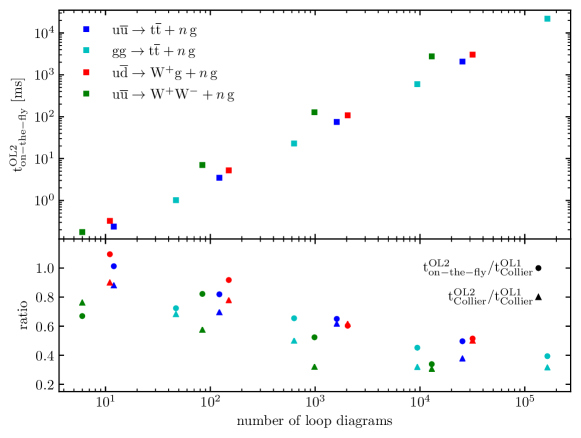
Refer to caption
Figure 13: Runtimes per phase space point for the calculation of the one-loop scattering probability (2.1) on a single Intel i7-4790K core with gfortran-4.8.5. Results for the processes in (LABEL:eq:proclist) are plotted versus the number of one-loop diagrams. Timings of OpenLoops 2 with on-the-fly reduction (ton-the-flyOL2subscriptsuperscript𝑡OL2on-the-flyt^{\text{OL2}}_{\text{on-the-fly}}) are shown in the upper frame. The lower frame presents a comparison to OpenLoops 2+Collier and OpenLoops 1+Collier (see Table 1).

6.2.1 Speed benchmarks

To illustrate the speed of the new algorithm, in Fig. 13 we plot runtimes per phase space point for the calculation of the one-loop scattering probability (2.1). The processes listed in (LABEL:eq:proclist) involve a number of one-loop Feynman diagrams that ranges from the order of 111 to 105superscript10510^{5}. The corresponding runtimes, measured on a single Intel i7-4790K core with gfortran-4.8.5, vary from the order of 101superscript10110^{-1} to 104superscript10410^{4} ms. In this range, we confirm that runtimes tend to grow linearly with the number of one-loop diagrams up to 24242\to 4 processes Cascioli:2011va , and we find that this scaling behaviour persists up to 25252\to 5 processes. As compared to OpenLoops 1+Collier, the new algorithm with on-the-fly reduction is up to a factor 2 to 3 faster for multi-particle processes. Depending on the process, using OpenLoops 2+Collier, i.e. restricting the on-the-fly approach to helicity sums plus diagram merging and reducing tensor integrals with Collier, can result in a further significant speed-up. However, the moderate slowdown caused by the on-the-fly reduction can be counterbalanced by the improved numerical stability, which implies a reduced need of re-evaluations in quadruple precision (see Section 6.2.2).

6.2.2 Stability benchmarks

In this section we study the numerical stability of the new open-loop algorithm. To this end, one-loop scattering probability densities computed in double precision (𝒲1loopDPsubscriptsuperscript𝒲DP1loop\mathcal{W}^{\scriptscriptstyle{\text{DP}}}_{\mathrm{1-loop}}) are compared against benchmarks in quadruple precision (𝒲1loopQPsubscriptsuperscript𝒲QP1loop\mathcal{W}^{\scriptscriptstyle{\text{QP}}}_{\mathrm{1-loop}}). More precisely, defining the relative difference between two results as

𝒜(𝒲a,𝒲b)𝒜subscript𝒲𝑎subscript𝒲𝑏\displaystyle\mathcal{A}(\mathcal{W}_{a},\mathcal{W}_{b}) =\displaystyle= log10|𝒲a𝒲b𝒲min|withsubscript10subscript𝒲𝑎subscript𝒲𝑏subscript𝒲with\displaystyle\log_{10}\left|\frac{\mathcal{W}_{a}-\mathcal{W}_{b}}{\mathcal{W}_{\min}}\right|\quad\mbox{with}
𝒲minsubscript𝒲\displaystyle\mathcal{W}_{\min} =\displaystyle= min{|𝒲a|,|𝒲b|},subscript𝒲𝑎subscript𝒲𝑏\displaystyle\min\left\{|\mathcal{W}_{a}|,|\mathcal{W}_{b}|\right\}, (159)

we estimate the instability of double-precision results as121212Note that, in order to avoid possible sources of bias, the quad-precision benchmark 𝒲1loopQP,Rsubscriptsuperscript𝒲QP,R1loop\mathcal{W}^{\scriptscriptstyle{\text{QP,R}}}_{\mathrm{1-loop}} is computed with rescaled kinematics as detailed below.

𝒜DP=𝒜(𝒲1loopDP,𝒲1loopQP,R).subscript𝒜DP𝒜subscriptsuperscript𝒲DP1loopsubscriptsuperscript𝒲QP,R1loop\mathcal{A}_{\scriptscriptstyle{\text{DP}}}=\mathcal{A}\left(\mathcal{W}^{\scriptscriptstyle{\text{DP}}}_{\mathrm{1-loop}},\mathcal{W}^{\scriptscriptstyle{\text{QP,R}}}_{\mathrm{1-loop}}\right). (160)

This quantity can be regarded, up to a minus sign, as the number of correct digits of the double-precision evaluation.
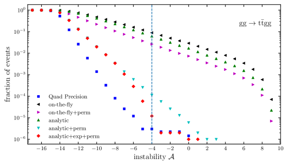
Refer to caption
Figure 14: Probability of finding events with instability 𝒜>𝒜min𝒜subscript𝒜min\mathcal{A}>\mathcal{A}_{\mathrm{min}} as a function of 𝒜minsubscript𝒜min\mathcal{A}_{\mathrm{min}} in a sample of 106superscript10610^{6} ggtt¯ggggt¯tgg\mathrm{gg}\to\mathrm{t\bar{t}gg} events. The stability of quad-precision benchmarks (blue) is compared to different variants of the OpenLoops 2 algorithm in double precision. Unstable results without special treatment of Gram determinants (“on-the-fly”) are stabilised using the permutation trick (144) for boxes (“perm”), exact analytic formulas for triangles (“analytic”) and Gram-determinant expansions for δ<δthr𝛿subscript𝛿thr\delta<\delta_{\mathrm{thr}} (“exp”). See Section 5.4.2.

To estimate the intrinsic accuracy of quad-precision benchmarks, computed using OpenLoops 1+Cuttools and OneLoop, we use a so-called rescaling test Badger:2010nx ; Cascioli:2011va , where scattering amplitudes are computed with rescaled masses and momenta and scaled back according to their mass dimensionality. Thus for a given phase space point the accuracy of the quadruple precision benchmarks is assessed as

𝒜QP=𝒜(𝒲1loopQP,𝒲1loopQP,R),subscript𝒜QP𝒜subscriptsuperscript𝒲QP1loopsubscriptsuperscript𝒲QP,R1loop\mathcal{A}_{\scriptscriptstyle{\text{QP}}}=\mathcal{A}\left(\mathcal{W}^{\scriptscriptstyle{\text{QP}}}_{\mathrm{1-loop}},\mathcal{W}^{\scriptscriptstyle{\text{QP,R}}}_{\mathrm{1-loop}}\right), (161)

where 𝒲1loopQPsubscriptsuperscript𝒲QP1loop\mathcal{W}^{\scriptscriptstyle{\text{QP}}}_{\mathrm{1-loop}} and 𝒲1loopQP,Rsubscriptsuperscript𝒲QP,R1loop\mathcal{W}^{\scriptscriptstyle{\text{QP,R}}}_{\mathrm{1-loop}} are the original and rescaled quad-precision evaluations. This quantity represents the finite resolution of the instability estimate (160). As we will see, quad-precision benchmarks can become more unstable than double-precision results obtained with OpenLoops 2. In this case, the instability estimate (160) yields 𝒜DP𝒜QPsimilar-tosubscript𝒜DPsubscript𝒜QP\mathcal{A}_{\scriptscriptstyle{\text{DP}}}\sim\mathcal{A}_{\scriptscriptstyle{\text{QP}}} but should be interpreted as 𝒜DP<𝒜QPsubscript𝒜DPsubscript𝒜QP\mathcal{A}_{\scriptscriptstyle{\text{DP}}}<\mathcal{A}_{\scriptscriptstyle{\text{QP}}}.

To assess the stability of OpenLoops 2, for each process in (LABEL:eq:proclist) we have studied a sample of 106superscript10610^{6} homogeneously distributed phase space points at s=1𝑠1\sqrt{s}=1 TeV. To exclude soft and collinear regions we have required pi,T>50subscript𝑝𝑖T50p_{i,\mathrm{T}}>50 GeV and ΔRij>0.5Δsubscript𝑅𝑖𝑗0.5\Delta R_{ij}>0.5 for all massless final-state QCD partons.

Fig. 14 illustrates the effect of Gram-determinant instabilities and the goodness of the solutions introduced in Section 5.4 in the case of ggtt¯ggggt¯tgg\mathrm{gg}\to\mathrm{t\bar{t}gg}. For this challenging multi-particle process, using the OpenLoops 2 on-the-fly reductions without any special treatment of Gram determinants we observe an extremely high level of numerical instability in double precision. The probabilities to obtain one-loop results with less than four or zero correct digits are around 101superscript10110^{-1} and 102superscript10210^{-2}, respectively, and the tail of the stability distribution extends up to a level of instability of ten orders of magnitude and more. Applying the permutation trick (144) (“perm”) and using analytic expressions for three-point integrals (“analytic”) result in a dramatic stability improvement for the box and triangle reductions, respectively. Combining these two improvements (“analytic+perm”) reduces the the probability of finding points with only few correct digits by three orders of magnitude, and yields a maximum level of instability around 102superscript10210^{2}. Finally, switching on the Gram-determinant expansions for δ<δthr𝛿subscript𝛿thr\delta<\delta_{\mathrm{thr}} leads to a further very drastic reduction of the probability of finding results with less than 3–4 correct digits. In this range, we observe an overlap with the tail of the quad-precision distribution. As discussed above, this indicates that OpenLoops 2 in double precision is more stable than the quad-precision benchmarks, and its estimated instability represents only an upper bound. Most likely, the tail of the true OpenLoops 2 stability distribution ends at 103superscript10310^{-3}.

on-the-fly Refer to caption

analytic + perm Refer to caption

analytic + perm + exp Refer to caption

Figure 15: Correlation between the instability 𝒜𝒜\mathcal{A} of OpenLoops 2 in double precision and the largest (Q4/Δ)2superscriptsuperscript𝑄4Δ2(Q^{4}/\Delta)^{2} in the event, where ΔΔ\Delta is any rank-two Gram determinant and Q2superscript𝑄2Q^{2} is the maximum scale in the corresponding Gram matrix. See (146). Probability densities correspond to 106superscript10610^{6} events. Unstable results without special treatment of Gram determinants (left) are stabilised using the permutation trick (144) for box reduction and analytic expressions for triangle reduction (middle) plus Gram-determinant expansions for δ<δthr𝛿subscript𝛿thr\delta<\delta_{\mathrm{thr}} (right).

To gain more insights into the origin of numerical instabilities in the on-the-fly reduction of OpenLoops 2, let us investigate the correlation between the instability (160) and rank-two Gram determinants ΔΔ\Delta in the ggtt¯ggggt¯tgg\mathrm{gg}\to\mathrm{t\bar{t}gg} sample of Fig. 14. More precisely, in Fig. 15 we consider the minimal value of the dimensionless parameter Δij/Qij4subscriptΔ𝑖𝑗superscriptsubscript𝑄𝑖𝑗4\Delta_{ij}/Q_{ij}^{4} in the event, where Qij2superscriptsubscript𝑄𝑖𝑗2Q_{ij}^{2} is the largest |pipj|subscript𝑝𝑖subscript𝑝𝑗|p_{i}\cdot p_{j}| in the corresponding Gram matrix (see Section 5.4.1). As demonstrated by the left plot in Fig. 15, the instability of the entire scattering amplitude features a remarkably strong correlation with rank-two Gram determinants over twenty orders of magnitude. Moreover we observe a quadratic or faster scaling in Q4/Δsuperscript𝑄4ΔQ^{4}/\Delta, consistent with the form of the γ2Δ2similar-tosuperscript𝛾2superscriptΔ2\gamma^{-2}\sim\Delta^{-2} poles in (5.2). The middle plot shows the combined effect of the permutation trick (144), which avoids the smallest Gram determinant of the event in all reductions with N4𝑁4N\geq 4 loop denominators, and the attenuation of spurious singularites through analytic expressions for three-point configurations of type (147). In this way the probability of having less than four correct digits is reduced to 0.1 permil. Finally, in the right plot we see that points with less than 3–4 correct digits disappear completely when Gram-determinant expansions are switched on.131313Points with unreliable quad-precision benchmarks (𝒜QP𝒜DPsimilar-tosubscript𝒜QPsubscript𝒜DP\mathcal{A}_{\scriptscriptstyle{\text{QP}}}\sim\mathcal{A}_{\scriptscriptstyle{\text{DP}}}) are not considered in Fig. 15. As one can clearly recognise in the right plot, the threshold for the activation of Gram-determinant expansions corresponds to (Q4/Δ)2δthr4=1012similar-tosuperscriptsuperscript𝑄4Δ2superscriptsubscript𝛿thr4superscript1012(Q^{4}/\Delta)^{2}\sim\delta_{\mathrm{thr}}^{-4}=10^{12}.

Finally, in Figs. 1617 we compare the stability of OpenLoops 2 against OpenLoops 1+Collier and OpenLoops 1+Cuttools for the 23232\to 3 and 24242\to 4 processes in (LABEL:eq:proclist). In OpenLoops 2 the stability improvements of Section 5.4 are applied throughout. The results of OpenLoops 1+Cuttools feature the highest instability tails for all considered processes. The probability of finding less than four correct digits can exceed 103superscript10310^{-3} in 23232\to 3 and 102superscript10210^{-2} in 24242\to 4 processes, while the fraction of fully unstable points with 𝒜0𝒜0\mathcal{A}\geq 0 can reach 103superscript10310^{-3} in 24242\to 4 processes. Switching to OpenLoops 1+Collier we find that, depending on the process, the probability of finding only a few correct digits goes down by one to three orders of magnitude, while in eight samples of 106superscript10610^{6} points we do not find a single result with 𝒜>0𝒜0\mathcal{A}>0.141414As discussed above, due to the insufficient quality of quad-precision benchmarks, instability estimates in the tail of ggtt¯ggggt¯tgg\mathrm{gg}\to\mathrm{t\bar{t}gg} are not significant.

Refer to caption
Refer to caption
Refer to caption
Refer to caption
Figure 16: Stability distributions for 23232\to 3 processes defined as in Fig. 14. The stability of OpenLoops 2 with on-the-fly reduction is compared to OpenLoops 1 with Collier or Cuttools. The instability of the employed quad precision benchmarks is also shown.
Refer to caption
Refer to caption
Refer to caption
Refer to caption
Figure 17: Stability distributions for 24242\to 4 processes defined as in Fig. 16.

Using OpenLoops 2 can lead to a further significant stability improvement. This is especially evident for 23232\to 3 processes, where the stability of the on-the-fly reduction in OpenLoops 2 is remarkably close to the quad-precision benchmarks and even superior than quad precision for the case of tt¯gt¯tg\mathrm{t\bar{t}g} production. When quad precision is sufficiently accurate to resolve the instabilities of OpenLoops 2 we observe improvements of one–two orders of magnitude with respect to OpenLoops 1+Collier. In the case of 24242\to 4 processes, depending on the process and the considered number of digits, OpenLoops 2 can perform somewhat better or slightly worse than OpenLoops 1+Collier, like in the case of ud¯W+gggu¯dsuperscriptWggg\mathrm{u\bar{d}}\to\mathrm{W^{+}ggg} or uu¯W+Wggu¯usuperscriptWsuperscriptWgg\mathrm{u\bar{u}}\to\mathrm{W^{+}W^{-}gg}, respectively. However, both approaches guarantee excellent numerical stability.

7 Conclusions and Outlook

We have presented a new approach for the automated calculation of scattering amplitudes at one loop. This new technique is based on the open-loop approach, where cut-open loop integrands are factored into a product of loop-momentum dependent segments that are combined through recursive tensorial multiplications.

The key idea behind the new method is that various operations, which are typically done at the level of full Feynman diagrams or amplitudes, can be performed on-the-fly during the open-loop recursion, i.e. after the multiplication of each loop segment. Since it exploits the factorised structure of open loops in a systematic way, this on-the-fly approach can reduce the complexity of certain operations in a very significant way.

We have first applied the on-the-fly method to helicity summations and to the merging of topologically equivalent open loops, finding speed-up factors of up to two or three as compared to the original open-loop algorithm. Moreover, using the integrand reduction method by del Aguila and Pittau, we have introduced an on-the-fly technique for the reduction of open loops. With this approach, the construction of loop amplitudes and their reduction are interleaved step by step within a single numerical recursion. In this way, objects with tensor rank higher than two are avoided throughout, and the complexity of the calculations is reduced in a very drastic way. The proliferation of pinched subtopologies that emerge from the reduction is avoided by absorbing them on-the-fly into topologically equivalent open loops.

The employed integrand reduction method suffers from severe numerical instabilities that are dominated by kinematic regions with small rank-two Gram determinants ΔΔ\Delta and scale like 1/Δ21superscriptΔ21/\Delta^{2}. In the reduction of N𝑁N-point objects with N4𝑁4N\geq 4, we have shown that ΔΔ\Delta-instabilities can easily be avoided through appropriate permutations of the loop denominators. In this way we were able to isolate ΔΔ\Delta-instabilities in triangle topologies with a particular kinematic configuration and to cure them by means of analytic expansions in ΔΔ\Delta. This approach is the first example of an integrand reduction algorithm that is essentially free from Gram-determinant instabilities. The level of stability that is achieved in double precision is competitive with public implementations of OPP reduction in quadruple precision.

The new algorithm is fully automated and validated at NLO QCD and can be extended to electroweak interactions. It will become publicly available in the upcoming release of OpenLoops 2. Its technical features can be especially beneficial in NLO calculations for challenging multi-particle processes. Moreover, in view of its excellent numerical stability, the new algorithm is very attractive for the calculation of real–virtual contributions at NNLO. Finally, the idea of simplifying the construction of loop amplitudes through the factorisation of loop integrands and their on-the-fly reduction may open new interesting perspectives for the automation of two-loop calculations.

Acknowledgments

We are grateful to P. Maierhöfer and J. Lindert for discussions and extensive technical support. This research was supported in part by the Swiss National Science Foundation (SNF) under contracts PP00P2-128552 and BSCGI0-157722 as well as by the Research Executive Agency (REA) of the European Union under the Grant Agreement PITN–GA–2012–316704 (HiggsTools).

Appendix A Reduction of the remaining tensor integrals

After the on-the-fly reduction described in Section 4.1 we are left with a few types of low-rank integrals ((ii)) that need to be reduced to the standard basis of one-loop scalar integrals. The relevant reductions are performed upon taking the trace (76) as described in the following. In this appendix we restrict ourselves to tensor integrals with four-dimensional qμsuperscript𝑞𝜇q^{\mu} terms in the numerator, while contributions with additional q~2superscript~𝑞2\tilde{q}^{2} terms in the numerator are described in Section 4.4.

A.1 Five- and higher-point integrals with R=0,1𝑅01R=0,1

Integrals with N5𝑁5N\geq 5 loop propagators and a numerator of rank R1𝑅1R\leq 1,

𝒩(q)=𝒩+𝒩μqμ,𝒩𝑞𝒩subscript𝒩𝜇superscript𝑞𝜇\displaystyle\mathcal{N}(q)=\mathcal{N}+\mathcal{N}_{\mu}q^{\mu}, (162)

can be reduced to a linear combination of scalar boxes,

dDq¯𝒩(q)D¯0D¯1D¯N1=superscriptd𝐷¯𝑞𝒩𝑞subscript¯𝐷0subscript¯𝐷1subscript¯𝐷𝑁1absent\displaystyle\int\!\mathrm{d}^{D}\!\bar{q}\,\frac{\mathcal{N}(q)}{\bar{D}_{0}\bar{D}_{1}\cdots\bar{D}_{N-1}}=
=i0<i1<i2<i3N1dDq¯di0i1i2i3D¯i0D¯i1D¯i2D¯i3.absentsuperscriptsubscriptsubscript𝑖0subscript𝑖1subscript𝑖2subscript𝑖3𝑁1superscriptd𝐷¯𝑞subscript𝑑subscript𝑖0subscript𝑖1subscript𝑖2subscript𝑖3subscript¯𝐷subscript𝑖0subscript¯𝐷subscript𝑖1subscript¯𝐷subscript𝑖2subscript¯𝐷subscript𝑖3\displaystyle=\sum_{i_{0}<i_{1}<i_{2}<i_{3}}^{N-1}\int\!\mathrm{d}^{D}\!\bar{q}\,\frac{d_{i_{0}i_{1}i_{2}i_{3}}}{\bar{D}_{i_{0}}\bar{D}_{i_{1}}\bar{D}_{i_{2}}\bar{D}_{i_{3}}}. (163)

To determine the box coefficients we use the OPP reduction formula Ossola:2006us

di0i1i2i3subscript𝑑subscript𝑖0subscript𝑖1subscript𝑖2subscript𝑖3\displaystyle d_{i_{0}i_{1}i_{2}i_{3}} =\displaystyle= 12[Ri0i1i2i3(q0+)+Ri0i1i2i3(q0)],12delimited-[]subscript𝑅subscript𝑖0subscript𝑖1subscript𝑖2subscript𝑖3superscriptsubscript𝑞0subscript𝑅subscript𝑖0subscript𝑖1subscript𝑖2subscript𝑖3superscriptsubscript𝑞0\displaystyle\frac{1}{2}\left[R_{i_{0}i_{1}i_{2}i_{3}}(q_{0}^{+})+R_{i_{0}i_{1}i_{2}i_{3}}(q_{0}^{-})\right],\quad (164)

where q0±superscriptsubscript𝑞0plus-or-minusq_{0}^{\pm} are the solutions of the quadruple-cut conditions D¯i0=D¯i1=D¯i2=D¯i3=0subscript¯𝐷subscript𝑖0subscript¯𝐷subscript𝑖1subscript¯𝐷subscript𝑖2subscript¯𝐷subscript𝑖30\bar{D}_{i_{0}}=\bar{D}_{i_{1}}=\bar{D}_{i_{2}}=\bar{D}_{i_{3}}=0, and

Ri0i1i2i3(q)=𝒩(q)ii0,i1,i2,i3N1D¯isubscript𝑅subscript𝑖0subscript𝑖1subscript𝑖2subscript𝑖3𝑞𝒩𝑞superscriptsubscriptproduct𝑖subscript𝑖0subscript𝑖1subscript𝑖2subscript𝑖3𝑁1subscript¯𝐷𝑖\displaystyle R_{i_{0}i_{1}i_{2}i_{3}}(q)=\frac{\mathcal{N}(q)}{\prod\limits_{i\neq i_{0},i_{1},i_{2},i_{3}}^{N-1}\bar{D}_{i}} (165)

are the corresponding residues.

For the special case d0123subscript𝑑0123d_{0123}, where pi0=p0=0subscript𝑝subscript𝑖0subscript𝑝00p_{i_{0}}=p_{0}=0, the explicit solutions of the quadruple cut equations read

q0±=x1l1+x2l2+x3±l4+x4±l4,superscriptsubscript𝑞0plus-or-minussubscript𝑥1subscript𝑙1subscript𝑥2subscript𝑙2superscriptsubscript𝑥3plus-or-minussubscript𝑙4superscriptsubscript𝑥4plus-or-minussubscript𝑙4q_{0}^{\pm}=x_{1}\,l_{1}+x_{2}\,l_{2}+x_{3}^{\pm}\,l_{4}+x_{4}^{\pm}\,l_{4}, (166)

where lisubscript𝑙𝑖l_{i} are the basis momenta defined in (119)(120). The x1,2subscript𝑥12x_{1,2} coefficients are given by

x1,2=1γ(d2,1d0(1α2,1)d1,2α2,1),subscript𝑥121𝛾subscript𝑑21subscript𝑑01subscript𝛼21subscript𝑑12subscript𝛼21\displaystyle x_{1,2}=\frac{1}{\gamma}\left(d_{2,1}-d_{0}\left(1-\alpha_{2,1}\right)-d_{1,2}\,\alpha_{2,1}\right),\qquad (167)

with di=mi2pi2subscript𝑑𝑖superscriptsubscript𝑚𝑖2superscriptsubscript𝑝𝑖2d_{i}=m_{i}^{2}-p_{i}^{2}. The terms α1,2subscript𝛼12\alpha_{1,2} and γ𝛾\gamma are defined in Section 5, and the remaining coefficients in (166) are given by

x4±=ax3±=(b±c0)2,superscriptsubscript𝑥4plus-or-minus𝑎superscriptsubscript𝑥3plus-or-minusplus-or-minus𝑏subscript𝑐02\displaystyle x_{4}^{\pm}=ax_{3}^{\pm}=-\frac{\left(b\pm c_{0}\right)}{2}, (168)

with a=(p3l3)/(p3l4)𝑎subscript𝑝3subscript𝑙3subscript𝑝3subscript𝑙4a=(p_{3}\cdot l_{3})/(p_{3}\cdot l_{4}) and

b𝑏\displaystyle b =\displaystyle= 1p3l4(d0d32+x1(p3l1)+x2(p3l2)),1subscript𝑝3subscript𝑙4subscript𝑑0subscript𝑑32subscript𝑥1subscript𝑝3subscript𝑙1subscript𝑥2subscript𝑝3subscript𝑙2\displaystyle\frac{1}{p_{3}\cdot l_{4}}\left(\frac{d_{0}-d_{3}}{2}+x_{1}\left(p_{3}\cdot l_{1}\right)+x_{2}\left(p_{3}\cdot l_{2}\right)\right),
c0subscript𝑐0\displaystyle c_{0} =\displaystyle= b2a(x1x2d0γ).superscript𝑏2𝑎subscript𝑥1subscript𝑥2subscript𝑑0𝛾\displaystyle\sqrt{b^{2}-a\left(x_{1}\,x_{2}-\frac{d_{0}}{\gamma}\right)}. (169)

The other coefficients di0i1i2i3subscript𝑑subscript𝑖0subscript𝑖1subscript𝑖2subscript𝑖3d_{i_{0}i_{1}i_{2}i_{3}} can be obtained from the above formulas through an obvious reparametrisation of masses and momenta (i0i1i2i30123subscript𝑖0subscript𝑖1subscript𝑖2subscript𝑖30123i_{0}i_{1}i_{2}i_{3}\to 0123) and a subsequent momentum shift, piμpiμp0μsuperscriptsubscript𝑝𝑖𝜇superscriptsubscript𝑝𝑖𝜇superscriptsubscript𝑝0𝜇p_{i}^{\mu}\to p_{i}^{\mu}-p_{0}^{\mu} for i=0,1,2,3𝑖0123i=0,1,2,3, which has to be applied throughout in (165)(169).

A.2 Four-point functions with R=1𝑅1R=1

The reduction of rank-one boxes,

dDq¯qμD¯0D¯3superscriptd𝐷¯𝑞superscript𝑞𝜇subscript¯𝐷0subscript¯𝐷3\displaystyle\int\!\mathrm{d}^{D}\!\bar{q}\,\frac{q^{\mu}}{\bar{D}_{0}\cdots\bar{D}_{3}} =\displaystyle= j=13dDq¯AjμD¯0D¯jD¯3,superscriptsubscript𝑗13superscriptd𝐷¯𝑞superscriptsubscript𝐴𝑗𝜇subscript¯𝐷0subscript¯𝐷𝑗subscript¯𝐷3\displaystyle\sum_{j=-1}^{3}\int\!\mathrm{d}^{D}\!\bar{q}\,\frac{A_{j}^{\mu}}{\bar{D}_{0}\cdots\not{\bar{D}_{j}}\cdots\bar{D}_{3}},\qquad\; (170)

results into a scalar box (j=1𝑗1j=-1) and four scalar triangles (j=0,1,2,3𝑗0123j=0,1,2,3). For the corresponding coefficients we use the reduction formulas delAguila:2004nf ,

A1,2μsubscriptsuperscript𝐴𝜇12\displaystyle A^{\mu}_{1,2} =\displaystyle= 12γ[r2,1μp3r2,1p3l3(l3μ+1αl4μ)],12𝛾delimited-[]subscriptsuperscript𝑟𝜇21subscript𝑝3subscript𝑟21subscript𝑝3subscript𝑙3subscriptsuperscript𝑙𝜇31𝛼subscriptsuperscript𝑙𝜇4\displaystyle\frac{1}{2\gamma}\left[r^{\mu}_{2,1}-\frac{p_{3}\cdot r_{2,1}}{p_{3}\cdot l_{3}}\left(l^{\mu}_{3}+\frac{1}{\alpha}l^{\mu}_{4}\right)\right],
A3μsubscriptsuperscript𝐴𝜇3\displaystyle A^{\mu}_{3} =\displaystyle= 141p3l3(l3μ+1αl4μ),141subscript𝑝3subscript𝑙3subscriptsuperscript𝑙𝜇31𝛼subscriptsuperscript𝑙𝜇4\displaystyle\frac{1}{4}\frac{1}{p_{3}\cdot l_{3}}\left(l^{\mu}_{3}+\frac{1}{\alpha}l^{\mu}_{4}\right), (171)

and

A1μ=i=13fi0Aiμ,A0μ=i=13Aiμ.formulae-sequencesubscriptsuperscript𝐴𝜇1superscriptsubscript𝑖13subscript𝑓𝑖0subscriptsuperscript𝐴𝜇𝑖subscriptsuperscript𝐴𝜇0superscriptsubscript𝑖13subscriptsuperscript𝐴𝜇𝑖\displaystyle A^{\mu}_{-1}=\sum_{i=1}^{3}f_{i0}A^{\mu}_{i},\qquad A^{\mu}_{0}=-\sum_{i=1}^{3}A^{\mu}_{i}. (172)

The relevant ingredients, γ,α,liμ,riμ,fi0𝛾𝛼subscriptsuperscript𝑙𝜇𝑖subscriptsuperscript𝑟𝜇𝑖subscript𝑓𝑖0\gamma,\alpha,l^{\mu}_{i},r^{\mu}_{i},f_{i0}, are defined in Section 5.

A.3 Three-point integrals with R=1𝑅1R=1

For rank-one triangles we use the covariant decomposition

Cμ(p1,p2,m0,m1,m2)=CεdDq¯qμD¯0D¯1D¯2=superscript𝐶𝜇subscript𝑝1subscript𝑝2subscript𝑚0subscript𝑚1subscript𝑚2subscript𝐶𝜀superscriptd𝐷¯𝑞superscript𝑞𝜇subscript¯𝐷0subscript¯𝐷1subscript¯𝐷2absent\displaystyle C^{\mu}(p_{1},p_{2},m_{0},m_{1},m_{2})=C_{{\varepsilon}}\int\!\mathrm{d}^{D}\!\bar{q}\,\frac{q^{\mu}}{\bar{D}_{0}\bar{D}_{1}\bar{D}_{2}}=
=i=12piμCi(p12,p22,m0,m1,m2),absentsuperscriptsubscript𝑖12superscriptsubscript𝑝𝑖𝜇subscript𝐶𝑖superscriptsubscript𝑝12superscriptsubscript𝑝22subscript𝑚0subscript𝑚1subscript𝑚2\displaystyle=\sum_{i=1}^{2}p_{i}^{\mu}C_{i}(p_{1}^{2},p_{2}^{2},m_{0},m_{1},m_{2}), (173)

where Cε=(2πμ)2ε/(iπ2)subscript𝐶𝜀superscript2𝜋𝜇2𝜀isuperscript𝜋2C_{{\varepsilon}}={(2\pi\mu)^{2{\varepsilon}}}/{(\mathrm{i}\pi^{2})}, and we compute the Cisubscript𝐶𝑖C_{i} coefficients via Passarino–Veltman reduction Passarino:1978jh ; Denner:1991kt .

A.4 Two-point integrals with R=1,2𝑅12R=1,2

Also for two-point integrals with rank R=1,2𝑅12R=1,2 we perform a Passarino–Veltman reduction Passarino:1978jh ; Denner:1991kt based on the covariant decomposition

Bμ(p1,m0,m1)superscript𝐵𝜇subscript𝑝1subscript𝑚0subscript𝑚1\displaystyle B^{\mu}(p_{1},m_{0},m_{1}) =\displaystyle= CεdDq¯qμD¯0D¯1=subscript𝐶𝜀superscriptd𝐷¯𝑞superscript𝑞𝜇subscript¯𝐷0subscript¯𝐷1absent\displaystyle C_{{\varepsilon}}\int\!\mathrm{d}^{D}\!\bar{q}\,\frac{q^{\mu}}{\bar{D}_{0}\bar{D}_{1}}= (174)
=\displaystyle= p1μB1(p12,m0,m1),superscriptsubscript𝑝1𝜇subscript𝐵1superscriptsubscript𝑝12subscript𝑚0subscript𝑚1\displaystyle p_{1}^{\mu}B_{1}(p_{1}^{2},m_{0},m_{1}),
Bμν(p1,m0,m1)superscript𝐵𝜇𝜈subscript𝑝1subscript𝑚0subscript𝑚1\displaystyle B^{\mu\nu}(p_{1},m_{0},m_{1}) =\displaystyle= CεdDq¯qμqνD¯0D¯1=subscript𝐶𝜀superscriptd𝐷¯𝑞superscript𝑞𝜇superscript𝑞𝜈subscript¯𝐷0subscript¯𝐷1absent\displaystyle C_{{\varepsilon}}\int\!\mathrm{d}^{D}\!\bar{q}\,\frac{q^{\mu}q^{\nu}}{\bar{D}_{0}\bar{D}_{1}}= (175)
=\displaystyle= p1μp1νB11(p12,m0,m1)superscriptsubscript𝑝1𝜇superscriptsubscript𝑝1𝜈subscript𝐵11superscriptsubscript𝑝12subscript𝑚0subscript𝑚1\displaystyle p_{1}^{\mu}p_{1}^{\nu}B_{11}(p_{1}^{2},m_{0},m_{1})
+\displaystyle+ gμνB00(p12,m0,m1).superscript𝑔𝜇𝜈subscript𝐵00superscriptsubscript𝑝12subscript𝑚0subscript𝑚1\displaystyle g^{\mu\nu}B_{00}(p_{1}^{2},m_{0},m_{1}).

Besides the standard reduction formulas for B1subscript𝐵1B_{1}, B11subscript𝐵11B_{11}, and B00subscript𝐵00B_{00}, for p2=0superscript𝑝20p^{2}=0 we have implemented the special cases

B1(0,m0,m0)subscript𝐵10subscript𝑚0subscript𝑚0\displaystyle B_{1}(0,m_{0},m_{0}) =\displaystyle= 12B0(0,m0,m0),12subscript𝐵00subscript𝑚0subscript𝑚0\displaystyle-\frac{1}{2}B_{0}(0,m_{0},m_{0}), (176)
B1(0,m0,m1)subscript𝐵10subscript𝑚0subscript𝑚1\displaystyle B_{1}(0,m_{0},m_{1}) =\displaystyle= 14(m02m12)(2A0(m1)\displaystyle\frac{1}{4(m_{0}^{2}-m_{1}^{2})}\Big{(}2A_{0}(m_{1}) (177)
2m02B0(0,m0,m1)1),\displaystyle-2m_{0}^{2}B_{0}(0,m_{0},m_{1})-1\Big{)},
B11(0,0,0)subscript𝐵11000\displaystyle B_{11}(0,0,0) =\displaystyle= 13B0(0,0,0)=0,13subscript𝐵00000\displaystyle\frac{1}{3}B_{0}(0,0,0)=0, (178)
B11(0,m0,m0)subscript𝐵110subscript𝑚0subscript𝑚0\displaystyle B_{11}(0,m_{0},m_{0}) =\displaystyle= 13+A0(m0)3m02,13subscript𝐴0subscript𝑚03superscriptsubscript𝑚02\displaystyle-\frac{1}{3}+\frac{A_{0}(m_{0})}{3m_{0}^{2}}, (179)
B11(0,m0,m1)subscript𝐵110subscript𝑚0subscript𝑚1\displaystyle B_{11}(0,m_{0},m_{1}) =\displaystyle= 118(m0m1)3(m0+m1)3118superscriptsubscript𝑚0subscript𝑚13superscriptsubscript𝑚0subscript𝑚13\displaystyle\frac{1}{18(m_{0}-m_{1})^{3}(m_{0}+m_{1})^{3}}
×(5m069m02m14+4m16+6m04A0(m0)\displaystyle\times\,\Big{(}5m_{0}^{6}-9m_{0}^{2}m_{1}^{4}+4m_{1}^{6}+6m_{0}^{4}A_{0}(m_{0})
6(3m043m02m12+m14)A0(m1)).\displaystyle\phantom{\times\,}-6(3m_{0}^{4}-3m_{0}^{2}m_{1}^{2}+m_{1}^{4})A_{0}(m_{1})\Big{)}.

with the scalar master integrals

B0(p12,m0,m1)subscript𝐵0superscriptsubscript𝑝12subscript𝑚0subscript𝑚1\displaystyle B_{0}(p_{1}^{2},m_{0},m_{1}) =\displaystyle= CεdDq¯1D¯0D¯1,subscript𝐶𝜀superscriptd𝐷¯𝑞1subscript¯𝐷0subscript¯𝐷1\displaystyle C_{{\varepsilon}}\int\!\mathrm{d}^{D}\!\bar{q}\,\frac{1}{\bar{D}_{0}\bar{D}_{1}},
A0(m02)subscript𝐴0superscriptsubscript𝑚02\displaystyle A_{0}(m_{0}^{2}) =\displaystyle= CεdDq¯1D¯0.subscript𝐶𝜀superscriptd𝐷¯𝑞1subscript¯𝐷0\displaystyle C_{{\varepsilon}}\int\!\mathrm{d}^{D}\!\bar{q}\,\frac{1}{\bar{D}_{0}}. (181)

References

  • (1) R. Britto, F. Cachazo and B. Feng, Generalized unitarity and one-loop amplitudes in N=4 super-Yang-Mills, Nucl. Phys. B725 (2005) 275–305, [hep-th/0412103].
  • (2) F. del Aguila and R. Pittau, Recursive numerical calculus of one-loop tensor integrals, JHEP 07 (2004) 017, [hep-ph/0404120].
  • (3) Z. Bern, L. J. Dixon and D. A. Kosower, Bootstrapping multi-parton loop amplitudes in QCD, Phys. Rev. D73 (2006) 065013, [hep-ph/0507005].
  • (4) A. Denner and S. Dittmaier, Reduction schemes for one-loop tensor integrals, Nucl. Phys. B734 (2006) 62–115, [hep-ph/0509141].
  • (5) G. Ossola, C. G. Papadopoulos and R. Pittau, Reducing full one-loop amplitudes to scalar integrals at the integrand level, Nucl. Phys. B763 (2007) 147–169, [hep-ph/0609007].
  • (6) D. Forde, Direct extraction of one-loop integral coefficients, Phys. Rev. D75 (2007) 125019, [0704.1835].
  • (7) W. T. Giele, Z. Kunszt and K. Melnikov, Full one-loop amplitudes from tree amplitudes, JHEP 04 (2008) 049, [0801.2237].
  • (8) A. van Hameren, Multi-gluon one-loop amplitudes using tensor integrals, JHEP 07 (2009) 088, [0905.1005].
  • (9) F. Cascioli, P. Maierhöfer and S. Pozzorini, Scattering Amplitudes with Open Loops, Phys.Rev.Lett. 108 (2012) 111601, [1111.5206].
  • (10) G. Ossola, C. G. Papadopoulos and R. Pittau, CutTools: A Program implementing the OPP reduction method to compute one-loop amplitudes, JHEP 03 (2008) 042, [0711.3596].
  • (11) C. F. Berger, Z. Bern, L. J. Dixon, F. Febres Cordero, D. Forde, H. Ita et al., An Automated Implementation of On-Shell Methods for One-Loop Amplitudes, Phys. Rev. D78 (2008) 036003, [0803.4180].
  • (12) A. van Hameren, C. G. Papadopoulos and R. Pittau, Automated one-loop calculations: A Proof of concept, JHEP 09 (2009) 106, [0903.4665].
  • (13) V. Hirschi, R. Frederix, S. Frixione, M. V. Garzelli, F. Maltoni and R. Pittau, Automation of one-loop QCD corrections, JHEP 05 (2011) 044, [1103.0621].
  • (14) P. Mastrolia, G. Ossola, T. Reiter and F. Tramontano, Scattering AMplitudes from Unitarity-based Reduction Algorithm at the Integrand-level, JHEP 08 (2010) 080, [1006.0710].
  • (15) S. Badger, B. Biedermann, P. Uwer and V. Yundin, Numerical evaluation of virtual corrections to multi-jet production in massless QCD, Comput. Phys. Commun. 184 (2013) 1981–1998, [1209.0100].
  • (16) F. Cascioli, J. M. Lindert, P. Maierhöfer and S. Pozzorini, The OpenLoops one-loop generator, Publicly available at http://openloops.hepforge.org .
  • (17) G. Cullen et al., GO𝑂\scriptsize{O}SAM𝐴𝑀\scriptsize{AM}-2.0: a tool for automated one-loop calculations within the Standard Model and beyond, Eur. Phys. J. C74 (2014) 3001, [1404.7096].
  • (18) T. Peraro, Ninja: Automated Integrand Reduction via Laurent Expansion for One-Loop Amplitudes, Comput. Phys. Commun. 185 (2014) 2771–2797, [1403.1229].
  • (19) A. Denner, S. Dittmaier and L. Hofer, Collier: a fortran-based Complex One-Loop LIbrary in Extended Regularizations, Comput. Phys. Commun. 212 (2017) 220–238, [1604.06792].
  • (20) S. Actis, A. Denner, L. Hofer, J.-N. Lang, A. Scharf and S. Uccirati, RECOLA: REcursive Computation of One-Loop Amplitudes, Comput. Phys. Commun. 214 (2017) 140–173, [1605.01090].
  • (21) T. Gleisberg, S. Hoeche, F. Krauss, M. Schonherr, S. Schumann, F. Siegert et al., Event generation with SHERPA 1.1, JHEP 02 (2009) 007, [0811.4622].
  • (22) S. Alioli, P. Nason, C. Oleari and E. Re, A general framework for implementing NLO calculations in shower Monte Carlo programs: the POWHEG BOX, JHEP 06 (2010) 043, [1002.2581].
  • (23) G. Bevilacqua, M. Czakon, M. V. Garzelli, A. van Hameren, A. Kardos, C. G. Papadopoulos et al., HELAC-NLO, Comput. Phys. Commun. 184 (2013) 986–997, [1110.1499].
  • (24) J. Alwall, R. Frederix, S. Frixione, V. Hirschi, F. Maltoni, O. Mattelaer et al., The automated computation of tree-level and next-to-leading order differential cross sections, and their matching to parton shower simulations, JHEP 07 (2014) 079, [1405.0301].
  • (25) T. Sjöstrand, S. Ask, J. R. Christiansen, R. Corke, N. Desai, P. Ilten et al., An Introduction to PYTHIA 8.2, Comput. Phys. Commun. 191 (2015) 159–177, [1410.3012].
  • (26) C. Weiss, B. Chokoufe Nejad, W. Kilian and J. Reuter, Automated NLO QCD Corrections with WHIZARD, PoS EPS-HEP2015 (2015) 466, [1510.02666].
  • (27) J. Bellm et al., Herwig 7.0/Herwig++ 3.0 release note, Eur. Phys. J. C76 (2016) 196, [1512.01178].
  • (28) Z. Bern, L. J. Dixon, F. Febres Cordero, S. Höche, H. Ita, D. A. Kosower et al., Next-to-Leading Order W+5𝑊5W+5-Jet Production at the LHC, Phys. Rev. D88 (2013) 014025, [1304.1253].
  • (29) S. Badger, B. Biedermann, P. Uwer and V. Yundin, Next-to-leading order QCD corrections to five jet production at the LHC, Phys. Rev. D89 (2014) 034019, [1309.6585].
  • (30) G. Bevilacqua, H. B. Hartanto, M. Kraus and M. Worek, Top Quark Pair Production in Association with a Jet with Next-to-Leading-Order QCD Off-Shell Effects at the Large Hadron Collider, Phys. Rev. Lett. 116 (2016) 052003, [1509.09242].
  • (31) S. Höche, P. Maierhöfer, N. Moretti, S. Pozzorini and F. Siegert, Next-to-leading order QCD predictions for top-quark pair production with up to three jets, Eur. Phys. J. C77 (2017) 145, [1607.06934].
  • (32) A. Denner, J.-N. Lang, M. Pellen and S. Uccirati, Higgs production in association with off-shell top-antitop pairs at NLO EW and QCD at the LHC, JHEP 02 (2017) 053, [1612.07138].
  • (33) F. Cascioli, S. Höche, F. Krauss, P. Maierhöfer, S. Pozzorini et al., Precise Higgs-background predictions: merging NLO QCD and squared quark-loop corrections to four-lepton + 0,1 jet production, JHEP 1401 (2014) 046, [1309.0500].
  • (34) F. Cascioli, P. Maierhöfer, N. Moretti, S. Pozzorini and F. Siegert, NLO matching for tt¯bb¯𝑡¯𝑡𝑏¯𝑏t\bar{t}b\bar{b} production with massive b𝑏b-quarks, Phys.Lett. B734 (2014) 210–214, [1309.5912].
  • (35) F. Cascioli, S. Kallweit, P. Maierhöfer and S. Pozzorini, A unified NLO description of top-pair and associated Wt production, Eur.Phys.J. C74 (2014) 2783, [1312.0546].
  • (36) S. Höche, F. Krauss, P. Maierhöfer, S. Pozzorini, M. Schönherr et al., Next-to-leading order QCD predictions for top-quark pair production with up to two jets merged with a parton shower, 1402.6293.
  • (37) S. Höche, F. Krauss, S. Pozzorini, M. Schönherr, J. Thompson et al., Triple vector boson production through Higgs-Strahlung with NLO multijet merging, Phys.Rev. D89 (2014) 093015, [1403.7516].
  • (38) T. Ježo, J. M. Lindert, P. Nason, C. Oleari and S. Pozzorini, An NLO+PS generator for tt¯𝑡¯𝑡t\bar{t} and Wt𝑊𝑡Wt production and decay including non-resonant and interference effects, Eur. Phys. J. C76 (2016) 691, [1607.04538].
  • (39) B. Chokoufé Nejad, W. Kilian, J. M. Lindert, S. Pozzorini, J. Reuter and C. Weiss, NLO QCD predictions for off-shell tt¯𝑡¯𝑡t\overline{t} and tt¯H𝑡¯𝑡𝐻t\overline{t}H production and decay at a linear collider, JHEP 12 (2016) 075, [1609.03390].
  • (40) S. Kallweit, J. M. Lindert, P. Maierhöfer, S. Pozzorini and M. Schönherr, NLO electroweak automation and precise predictions for W+multijet production at the LHC, JHEP 04 (2015) 012, [1412.5157].
  • (41) S. Kallweit, J. M. Lindert, P. Maierhofer, S. Pozzorini and M. Schönherr, NLO QCD+EW predictions for V + jets including off-shell vector-boson decays and multijet merging, JHEP 04 (2016) 021, [1511.08692].
  • (42) S. Kallweit, J. M. Lindert, S. Pozzorini and M. Schonherr, NLO QCD+EW predictions for 22ν22𝜈2\ell 2\nu diboson signatures at the LHC, 1705.00598.
  • (43) J. M. Lindert et al., Precise predictions for V+jets dark matter backgrounds, 1705.04664.
  • (44) F. Granata, J. M. Lindert, C. Oleari and S. Pozzorini, NLO QCD+EW predictions for HV and HV +jet production including parton-shower effects, JHEP 09 (2017) 012, [1706.03522].
  • (45) M. Wiesemann, M. Grazzini, S. Kallweit and D. Rathlev, Fully-differential NNLO predictions for vector-boson pair production with MATRIX, PoS LL2016 (2016) 072.
  • (46) M. Grazzini, S. Kallweit, D. Rathlev and A. Torre, Zγ𝑍𝛾Z\gamma production at hadron colliders in NNLO QCD, Phys.Lett. B731 (2014) 204–207, [1309.7000].
  • (47) F. Cascioli, T. Gehrmann, M. Grazzini, S. Kallweit, P. Maierhöfer et al., ZZ production at hadron colliders in NNLO QCD, Phys.Lett. B735 (2014) 311–313, [1405.2219].
  • (48) T. Gehrmann, M. Grazzini, S. Kallweit, P. Maierhöfer, A. von Manteuffel et al., W+Wsuperscript𝑊superscript𝑊W^{+}W^{-} Production at Hadron Colliders in Next to Next to Leading Order QCD, Phys.Rev.Lett. 113 (2014) 212001, [1408.5243].
  • (49) M. Grazzini, S. Kallweit and D. Rathlev, Wγ𝑊𝛾W\gamma and Zγ𝑍𝛾Z\gamma production at the LHC in NNLO QCD, JHEP 07 (2015) 085, [1504.01330].
  • (50) M. Grazzini, S. Kallweit, D. Rathlev and M. Wiesemann, Transverse-momentum resummation for vector-boson pair production at NNLL+NNLO, JHEP 08 (2015) 154, [1507.02565].
  • (51) M. Grazzini, S. Kallweit and D. Rathlev, ZZ production at the LHC: fiducial cross sections and distributions in NNLO QCD, Phys. Lett. B750 (2015) 407–410, [1507.06257].
  • (52) M. Grazzini, S. Kallweit, D. Rathlev and M. Wiesemann, W±Zsuperscript𝑊plus-or-minus𝑍W^{\pm}Z production at hadron colliders in NNLO QCD, 1604.08576.
  • (53) M. Grazzini, S. Kallweit, S. Pozzorini, D. Rathlev and M. Wiesemann, W+Wsuperscript𝑊superscript𝑊W^{+}W^{-} production at the LHC: fiducial cross sections and distributions in NNLO QCD, 1605.02716.
  • (54) D. de Florian, M. Grazzini, C. Hanga, S. Kallweit, J. M. Lindert, P. Maierhöfer et al., Differential Higgs Boson Pair Production at Next-to-Next-to-Leading Order in QCD, JHEP 09 (2016) 151, [1606.09519].
  • (55) M. Grazzini, S. Kallweit, D. Rathlev and M. Wiesemann, W±Zsuperscript𝑊plus-or-minus𝑍W^{\pm}Z production at the LHC: fiducial cross sections and distributions in NNLO QCD, 1703.09065.
  • (56) A. Bredenstein, A. Denner, S. Dittmaier and S. Pozzorini, NLO QCD Corrections to Top Anti-Top Bottom Anti-Bottom Production at the LHC: 2. full hadronic results, JHEP 03 (2010) 021, [1001.4006].
  • (57) J. A. M. Vermaseren, Axodraw, Comput. Phys. Commun. 83 (1994) 45–58.
  • (58) F. A. Berends and W. T. Giele, Recursive Calculations for Processes with n Gluons, Nucl. Phys. B306 (1988) 759–808.
  • (59) G. Ossola, C. G. Papadopoulos and R. Pittau, On the Rational Terms of the one-loop amplitudes, JHEP 05 (2008) 004, [0802.1876].
  • (60) P. Draggiotis, M. V. Garzelli, C. G. Papadopoulos and R. Pittau, Feynman Rules for the Rational Part of the QCD 1-loop amplitudes, JHEP 04 (2009) 072, [0903.0356].
  • (61) M. V. Garzelli, I. Malamos and R. Pittau, Feynman rules for the rational part of the Electroweak 1-loop amplitudes, JHEP 01 (2010) 040, [0910.3130].
  • (62) R. Pittau, Primary Feynman rules to calculate the epsilon-dimensional integrand of any 1-loop amplitude, JHEP 02 (2012) 029, [1111.4965].
  • (63) A. Denner and S. Dittmaier, Reduction of one-loop tensor 5-point integrals, Nucl. Phys. B658 (2003) 175–202.
  • (64) A. Denner and S. Dittmaier, Scalar one-loop 4-point integrals, Nucl. Phys. B844 (2011) 199–242.
  • (65) A. van Hameren, OneLOop: For the evaluation of one-loop scalar functions, Comput.Phys.Commun. 182 (2011) 2427–2438, [1007.4716].
  • (66) A. Denner, S. Dittmaier and L. Hofer, COLLIER – A fortran-library for one-loop integrals, 1407.0087.
  • (67) R. N. Lee, LiteRed 1.4: a powerful tool for reduction of multiloop integrals, J. Phys. Conf. Ser. 523 (2014) 012059, [1310.1145].
  • (68) T. Hahn, Generating Feynman diagrams and amplitudes with FeynArts 3, Comput. Phys. Commun. 140 (2001) 418–431, [hep-ph/0012260].
  • (69) S. Badger, B. Biedermann and P. Uwer, NGluon: A Package to Calculate One-loop Multi-gluon Amplitudes, Comput. Phys. Commun. 182 (2011) 1674–1692, [1011.2900].
  • (70) G. Passarino and M. J. G. Veltman, One Loop Corrections for e+ e- Annihilation Into mu+ mu- in the Weinberg Model, Nucl. Phys. B160 (1979) 151–207.
  • (71) A. Denner, Techniques for calculation of electroweak radiative corrections at the one loop level and results for W physics at LEP-200, Fortsch. Phys. 41 (1993) 307–420, [0709.1075].