A Scaled Smart City for Experimental Validation of Connected and Automated Vehicles
Abstract
The common thread that characterizes energy-efficient mobility systems for smart cities is their interconnectivity which enables the exchange of massive amounts of data. This, in turn, provides the opportunity to develop a decentralized framework to process this information and deliver real-time control actions that optimize energy consumption and other associated benefits. To seize these opportunities, this paper describes the development of a scaled smart city providing a glimpse that bridges the gap between simulation and full scale implementation of energy-efficient mobility systems. Using this testbed, we can quickly, safely, and affordably experimentally validate control concepts aimed at enhancing our understanding of the implications of next generation mobility systems.
keywords:
Smart cities, connected and automated vehicles, vehicle coordination, cooperative merging control.1 Introduction
In a rapidly urbanizing world, we need to make fundamental transformations in how we use and access transportation. Energy-efficient mobility systems such as Connected and Automated Vehicles along with shared mobility and electric vehicles provide the most intriguing and promising opportunities for enabling users to better monitor transportation network conditions and make better operating decisions to reduce energy consumption, greenhouse gas emissions, travel delays and improve safety. As we move to increasingly complex transportation systems new control approaches are needed to optimize the system behavior resulting from the interactions between vehicles navigating different traffic scenarios.
Given this new environment, the overarching goal of this paper is to (1) report on the development of the University of Delaware Scaled Smart City (UDSSC) testbed that includes 35 robotic cars to replicate real-world traffic scenarios in a small and controlled environment, and (2) use this testbed to demonstrate CAV coordination at merging roadways. UDSSC can serve as a testbed to explore the acquisition and processing of vehicle-to-vehicle and vehicle-to-infrastructure communication. It can also help us prove control concepts on coordinating CAVs in specific transportation scenarios, e.g., intersections, merging roadways, roundabouts, speed reduction zones, etc. These scenarios along with the driver responses to various disturbances are the primary sources of bottlenecks that contribute to traffic congestion; see Margiotta and Snyder (2011); Malikopoulos and Aguilar (2013). In 2015, congestion caused people in urban areas in the US to spend 6.9 billion additional hours on the road and to purchase an extra 3.1 billion gallons of fuel, resulting in a total cost estimated at $160 billion; see Schrank et al. (2015).
CAVs can provide shorter gaps between vehicles and faster responses while improving highway capacity. Several research efforts have been reported in the literature proposing either centralized or decentralized approaches for coordinating CAVs in specific traffic scenarios. The overarching goal of such efforts is to yield a smooth traffic flow avoiding stop-and-go driving. Numerous approaches have been reported in the literature on coordinating CAVs in different transportation scenarios with the intention of improving traffic flow. Kachroo and Li (1997) proposed a longitudinal and lateral controller to guide the vehicle until the merging maneuver is completed. Other efforts have focused on developing a hybrid control aimed at keeping a safe headway between vehicles in the merging process, see Kachroo and Li (1997); Antoniotti et al. (1997); or developing three levels of assistance for the merging process to select a safe space for the vehicle to merge; see Ran et al. (1999). Some authors have explored virtual vehicle platooning, where a controller identifies and interchanges appropriate information between the vehicles involved in the merging maneuver while each vehicle assumes its own control actions to satisfy the assigned time and reference speed; see Lu et al. (2000).
VanMiddlesworth et al. (2008) addressed the problem of traffic coordination for small intersections which commonly handle low traffic loads. Milanés et al. (2010) designed a controller that allows a fully automated vehicle to yield to an incoming vehicle in the conflicting road or to cross, if it is feasible without the risk of collision. Alonso et al. (2011) proposed two conflict resolution schemes in which an autonomous vehicle could make a decision about the appropriate crossing schedule and trajectory to follow to avoid collision with other manually driven vehicles on the road. A survey of the research efforts in this area that have been reported in the literature to date can be found in Rios-Torres and Malikopoulos (2017a).
Although previous work has shown promising results emphasizing the potential benefits of coordination between CAVs, validation has been primarily in simulation. In this paper, we demonstrate coordination of scaled CAVs and quantify the benefits in energy usage. The contributions of this paper are: 1) the development of a 1:25 scaled smart city capable of testing decentralized control algorithms on up to 35 Micro Connected and Automated Vehicles and 2) the experimental validation of a control framework reported in Rios-Torres and Malikopoulos (2017b) for coordination of CAVs.
The remainder of the paper proceeds as follows. In Section II, we introduce the configurations of UDSSC. In Section III, we review a decentralized control framework for coordination of CAVs in merging roadways. Experimental results in Section IV illustrate the effectiveness of the proposed solution in the scaled smart city environment. We draw concluding remarks in Section V.
2 University of Delaware Scaled Smart City (UDSSC)
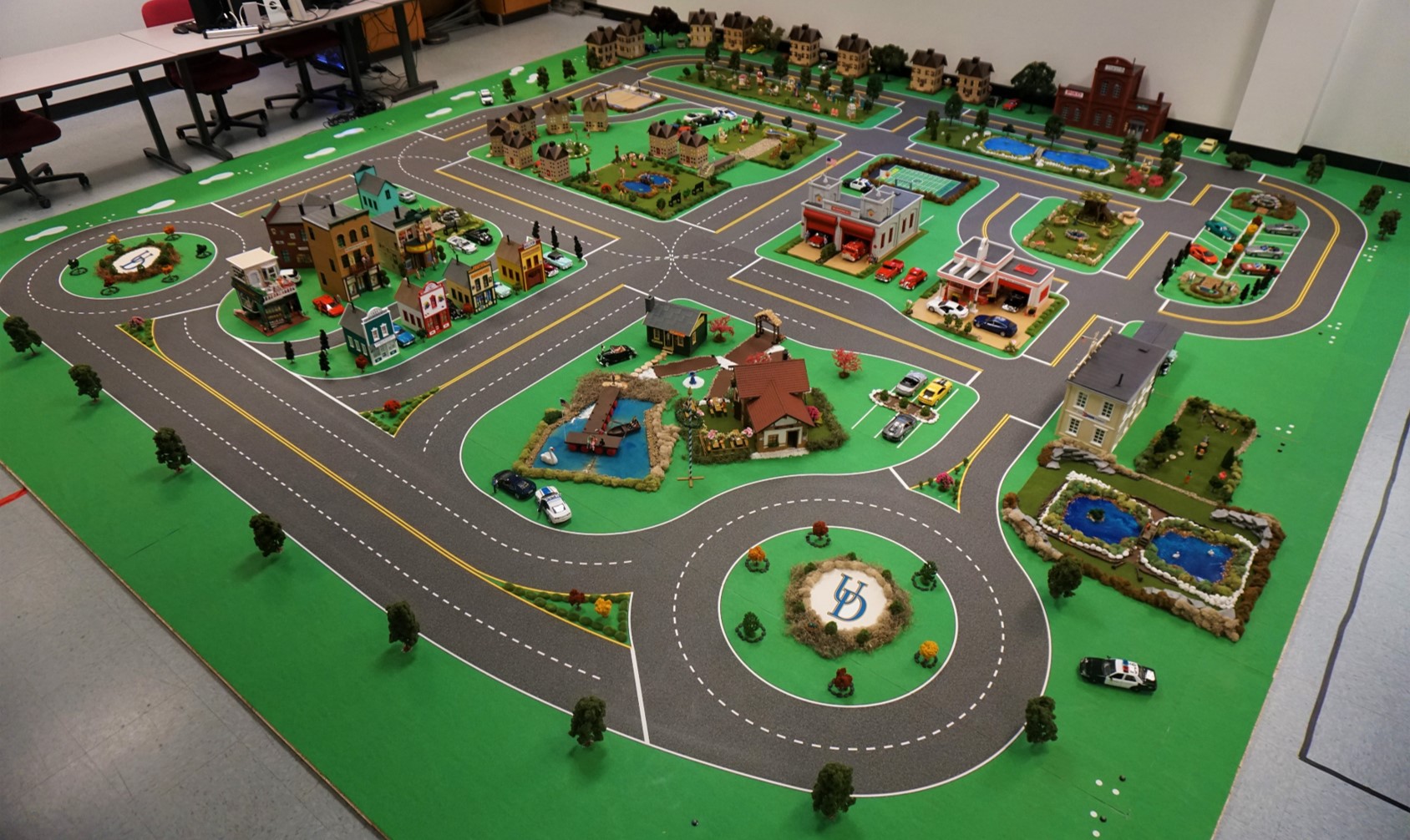
UDSSC is a testbed that can replicate real-world traffic scenarios in a small, controlled environment and help formulate the appropriate features of a “smart” city. It can be used as an effective way to visualize the concepts developed using CAVs and their related implications in energy usage. UDSSC is a fully integrated smart city (Fig. 1) incorporating realistic environmental cues, scaled MCAVs, and state-of-the-art, high-end computers supporting standard software for system analysis and optimization for simulating different control algorithms and distributing control inputs to as many as 35 MCAVs.
2.1 Physical Design I: Map
The UDSSC spans over 400 square feet and includes one lane intersections, two lane intersections, roundabouts, and a highway with entrance and exit ramps. Using SolidWorks to accurately maintain 1:25 scale, a fully dimensioned blueprint was designed forming a cohesive roadway representative of real world road scenarios. Using a HP DesignJet z5200 printer the map is printed with realistic texturing on twelve 44”x120” sheets of wear resistant HP Artist Matte Canvas that can be easily replaced to either reconfigure or repair sections of the city independently. Eight Vicon Vantage V16 cameras are used to localize the map within a global coordinate system.
2.2 Physical Design II: Cars
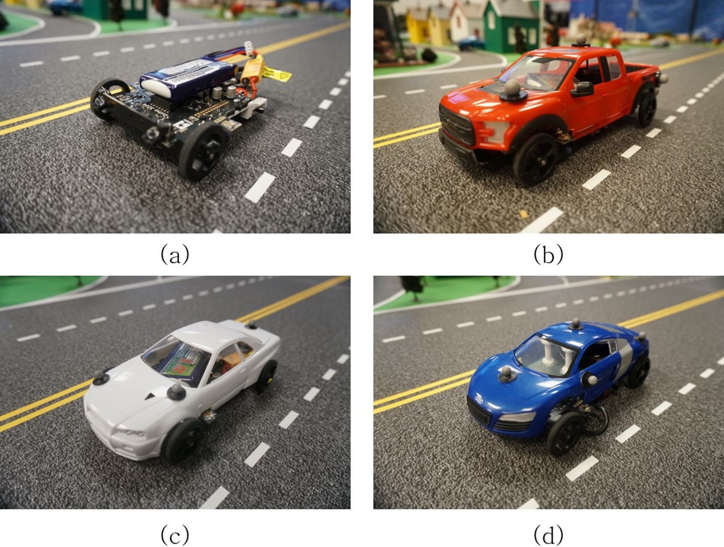
Scaled MCAVs have been designed using easily assembled off-the-shelf components coupled with several 3D printed parts (Fig. 2). At the core of each platform is a 75.81:1 geared, differentially driven Pololu Zumo, offering dual H-bridge motor drivers, counts per revolution (CPR) encoders and an on-board Atmega 32U4 micro-controller. Each Zumo contains an embedded set of sensors including an IMU, line-following, and infrared proximity sensors which can provide feedback to each MCAV. Rubberized wheels with radius are mounted directly to each gear motor output shaft and separated by to roughly mimic the 1:25 scale width of full sized cars/trucks. The Zumo is connected to an on-board Raspberry Pi 3 with 1.2 GHz quad-core ARM Cortex A53 micro-processor and WiFi used for communication. The MCAV platform (not including its car-shaped shell) measures x x . A power regulator manages the voltage requirements of the Raspberry Pi 3, supplying a regulated 5VDC from a 7.4VDC, 1000mAh Li-Po battery. Fully charged MCAVs are capable of running approximately 90 minutes before being recharged.
2.3 Control System Architecture
UDSSC has a multi-level control architecture with high level commands originating from a centralized PC called the “Main Frame” (Processor: Intel Core i7-6950X CPU @ 3.00 GHz x 20, Memory: 125.8 GiB) then enforced by a low-level controller on-board each MCAV. Asynchronous communication is enabled by WiFi connectivity using the Node.js non-blocking I/O protocol. Electron uses the socketIO library supporting multi-threading for multi-vehicle communication. A web browser combines JavaScript, HTML, and CSS for a user friendly interface into the Robot Operating System (ROS) architecture. Generally control of each MCAV can be broken into merging, lane and reference tracking controllers, the latter two of which enforce realistic road behaviors (i.e. staying in the center of the road and respecting speed limits.)
2.3.1 Lane tracking:
The roads of UDSSC are encoded as sequences of tangent arcs and straight line segments each with an associated potential field. Potential field methods provide important computational expedience due to their analytical representation. Given a looping sequence of road segments an MCAV starting on the first road segment will follow along the road until its battery is depleted. Although an MCAV can use lane tracking directly to follow along a road, while in the control region merging requires a carefully maintained velocity profile with respect to the lane center. Offsets from the centerline of the lane using lane tracking results in noisy forward velocity measurements, however a virtual robot can track the center of each lane exactly. For situations where precise velocity profiles are required, instead of controlling each MCAV using the potential field directly a virtual robot is simulated within the vector field and used as a reference point tracked by the real robot.
2.3.2 Reference tracking:
As long as a reference point tracks a sequence of road segments using lane tracking, an MCAV can be controlled by reference tracking. A state tracking method as described in Giuseppe and Vendittelli (2002) is used, approximately linearizing the error dynamics of the MCAV’s local frame with respect to a reference trajectory.
2.3.3 Merging scenario:
There have been several approaches for automated vehicle merging as reported in Rios-Torres and Malikopoulos (2017a). In this paper, we consider the control approach described in Section 3 with the Main Frame tracking the positions of each MCAV in order to determine when vehicles enter the control zones. Once inside the control zone a virtual robot tracks the desired velocity profile exactly and reference tracking is used to mimic this behavior by the associated MCAV.
2.3.4 Low level control:
In place of car-like models which would require a more complex mechanical design, Zumo based MCAVs are differentially driven. Practically the control input is expressed as with and representing the forward and angular velocities respectively. On-board encoders enable low-level control from wirelessly transmitted inputs, converted into independent wheel velocities by two relationships: and with as the right and left wheels angular velocity respectively and as wheel radius. High frequency control results in noisy measurements due to low-resolution encoders. The Atmega 32U4 measures encoder pulses at a frequency of 2 kHz then smooths the velocity estimate by averaging a 25 measurement queue. A proportional controller adjusts the PWM duty cycle depending on the error between measured and desired velocity, saturating at 0.7m/s 0.1m/s depending on transmission friction and slight variations between MCAVs.
3 Coordination of Connected and Automated Vehicles
3.1 Modeling Framework
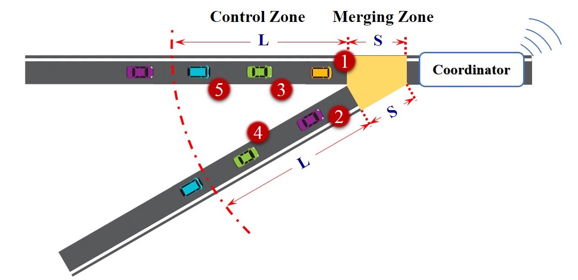
We consider a merging roadway (Fig. 3) consisting of main and secondary roads. The region where lateral collision between vehicles can occur is called merging zone and has a length of . On each road, there is a control zone inside of which all vehicles can communicate with each other and with a coordinator. Note that the coordinator is not involved in any decision for any CAV and only enables communication of appropriate information among CAVs. The distance from the entry of the control zone to the entry of the merging zone is . The value of depends on the communication range between CAVs and the coordinator, and is the physical length of a merging zone.
Let be the number of CAVs inside the control zone at time and be a queue designating the order in which these vehicles enter the merging zone. Thus, letting be the assigned time for vehicle to enter the merging zone, we require that
| (1) |
There are a number of ways to satisfy (1). For example, we may impose a strict First-in-First-Out (FIFO) queuing structure, where each vehicle must enter the merging zone in the same order it entered the control zone. We investigate a specific scheme for determining (upon arrival of CAV ) based on our problem formulation, without affecting , but emphasize that our analysis is not restricted by the policy designating the order of the vehicles within the queue .
We adopt the optimization framework proposed in Rios-Torres and Malikopoulos (2017b) for coordinating the merging of CAVs. The dynamics of each vehicle are represented by a double integrator,
| (2) |
where is the time, , , and denotes position, speed and acceleration/deceleration (control input) of each vehicle inside the control zone. Let denote the state of each vehicle , with initial value . The state space is closed with respect to the induced topology, thus, it is compact.
For any initial state , where is the time that the vehicle enters the control zone, and every admissible control , the double integrator has a unique solution on some interval , where is the time that vehicle enters the merging zone. In our framework we impose the following state and control constraints:
| (3) |
where , are the minimum and maximum control inputs (maximum deceleration/acceleration) for each vehicle , and , are the minimum and maximum speed limits respectively. For simplicity, in the rest of the paper we consider no vehicle diversity, and thus, we set and .
For absence of any rear-end collision of two consecutive vehicles traveling on the same lane, the position of the preceding vehicle should be greater than or equal to the position of the following vehicle plus a safe distance , which is a function of the average speed of the vehicles inside the control zone. Thus, we impose the following rear-end safety constraint
| (4) |
where denotes the vehicle that is physically located ahead of in the same lane, and is the average speed of the vehicles inside the control zone at time .
Definition 1
Each CAV belongs to at least one of the following two subsets of depending on its physical location inside the control zone: 1) contains all CAVs traveling on the same road and lane as vehicle and 2) contains all CAVs traveling on a different road from and can cause collision at the merging zone.
Definition 2
For each vehicle , we define the set that includes only the positions along the lane where a lateral collision is possible, namely
| (5) |
with as the time vehicle exits the merging zone.
Consequently, to avoid a lateral collision for any two vehicles on different roads, the following constraint should hold
| (6) |
The above constraint implies that only one vehicle at a time can be inside the merging zone. If the length of the merging is long, then this constraint may not be realistic since it results in dissipating space and capacity of the road. However, the constraint is not restrictive in the problem formulation and it can be modified appropriately.
In the modeling framework described above, we impose the following assumptions:
Assumption 1
The vehicles cruise inside the merging zone with an imposed speed limit, . This implies that for each vehicle
| (7) |
This assumption is intended to enhance safety awareness, but it could be modified appropriately, if necessary.
3.2 Communication Structure of Connected and Automated Vehicles
We consider the problem of deriving the optimal control input (acceleration/deceleration) of each CAV inside the control zone (Fig. 3), under the hard safety constraints to avoid rear-end and lateral collision. By controlling the speed of the vehicles, the speed of the queue built-up at the merging zone decreases, and thus the congestion recovery time is also reduced. The latter results in maximizing the throughput in the merging zone.
When a CAV enters the control zone, it can communicate with the other CAVs in the control zone and with the coordinator. Note that the coordinator is not involved in any decision for any CAV and only enables communication of appropriate information among CAVs. The coordinator handles the information between the vehicles as follows. When a CAV reaches the control zone at some instant , the coordinator assigns a unique identity to each vehicle which is a pair , where is an integer representing the location of the vehicle in a FIFO queue and is an integer based on a one-to-one mapping from and onto . If the vehicles enter the control zone at the same time, then the coordinator selects randomly their position in the queue.
Definition 3
For each CAV entering the control zone, we define the information set which includes all information that each vehicle shares, as
| (8) |
where are the position and speed of CAV inside the control zone, is the subset assigned to CAV by the coordinator, and , is the target time for CAV to enter the merging zone.
The time that vehicle will be entering the merging zone is restricted by imposing rear-end and lateral collision constraints. Therefore, to ensure (4) and (6) are satisfied at we impose the following conditions which depend on the subset vehicle belongs to. If
| (9) |
and if
| (10) |
where , is the imposed speed inside the merging zone (Assumption 1), and is the initial speed of vehicle when it enters the control zone at . The conditions (9) and (10) ensure the time each vehicle will be entering the merging zone is feasible and can be attained based on the imposed speed limits inside the control zone. In addition, for low traffic flow where vehicle and might be located far away from each other, there is no compelling reason for vehicle to accelerate within the control zone to maintain a distance from vehicle . Therefore, in such cases vehicle can keep cruising within the control zone with the initial speed that entered the control zone at
The recursion is initialized when the first vehicle enters the control zone and is assigned . In this case, can be externally assigned as the desired exit time of this vehicle whose behavior is unconstrained. Thus the time is fixed and available through . The second vehicle accesses to compute time . The third vehicle accesses and the communication process continues in the same fashion until vehicle in the queue accesses .
3.3 Optimal Control Problem Formulation for CAVs
Since the coordinator is not involved in any decision on the vehicle coordination we can formulate sequential decentralized control problems that may be solved on-line:
| (11) | |||
with initial and final conditions: , , and . In (11), rear end (4) and lateral (6) collision safety constraints are omitted. As mentioned earlier, (6) implicitly handled by the selection of in (10). Eq. (4) is omitted because it has been shown Malikopoulos et al. (2018) that the solution of (11) guarantees this constraint holds throughout . Thus, (11) is a simpler problem to solve on-line.
4 Experimental Results
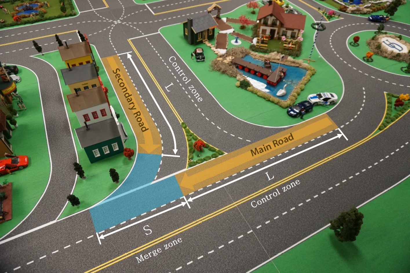
To evaluate the effectiveness and efficiency of the proposed approach, a total number of ten MCAVs are set up in a merging scenario [video available in Stager (2017)]. Five MCAVs cruise on the main road in UDSSC, while the other five MCAVs cruise on the secondary road with the intention to merge into the main road (Fig. 4).
We consider two scenarios: 1) all MCAVs are controlled by the decentralized control algorithm; 2) all MCAVs behave based on a simple (baseline) car following model, with MCAVs on the secondary road yielding to MCAVs of the main road to avoid lateral collision in the merging zone.
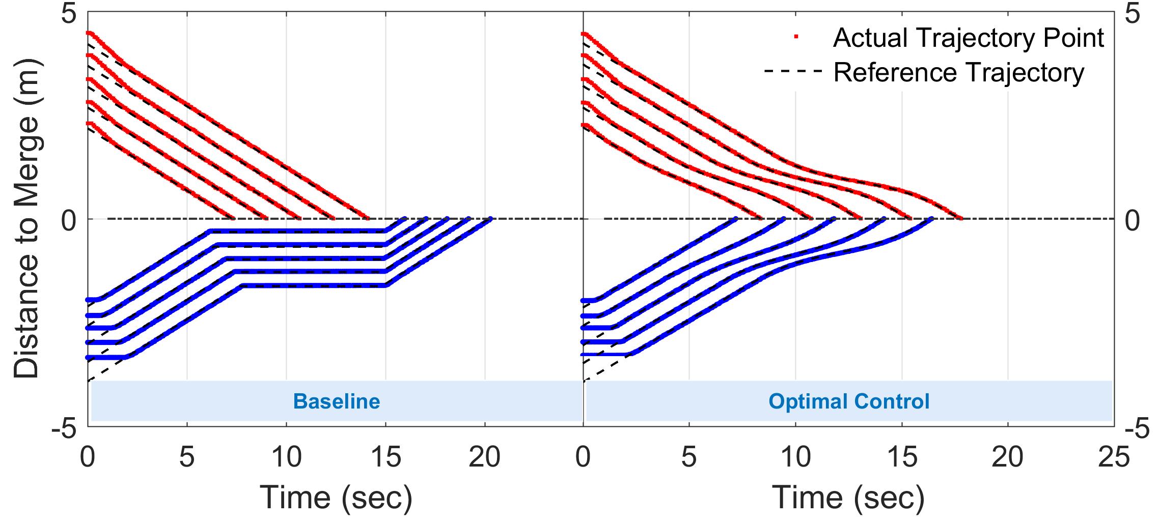
4.0.1 Vehicle Position Trajectory:
Position trajectories of MCAVs under two scenarios are illustrated in Fig. 5. A dashed line represents the reference trajectory for each vehicle commanded by the control algorithm, while a dense scatter plot represents points measured along the actual trajectory achieved by each MCAV. To separate the MCAVs on two roads, trajectories are flipped over Y-axis. Thus, in Fig. 5, red dots stand for trajectory points of the MCAVs on the main road, and blue dots stand for the trajectory points of MCAVs on the secondary road. On the right panel of Fig. 5, MCAVs follow the optimal trajectory and merge successfully without stop-and-go driving with only marginal errors. Position trajectories of MCAVs cruising without the optimal control (baseline scenario) are shown in the left panel of Fig. 5. Since the gaps between the mainline cars are not large enough for merging cars to safely merge into the roadway, merging cars need to stop until all leading mainline vehicles traverse the merging zone, resulting in queuing on the merging roadway. For comparison, the merging maneuver for all ten cars is completed in 16.5 sec with the optimal control algorithm, whereas it takes 20.3 sec for the baseline (i.e. an 18.7% travel time savings is achieved with the optimal control algorithm.)
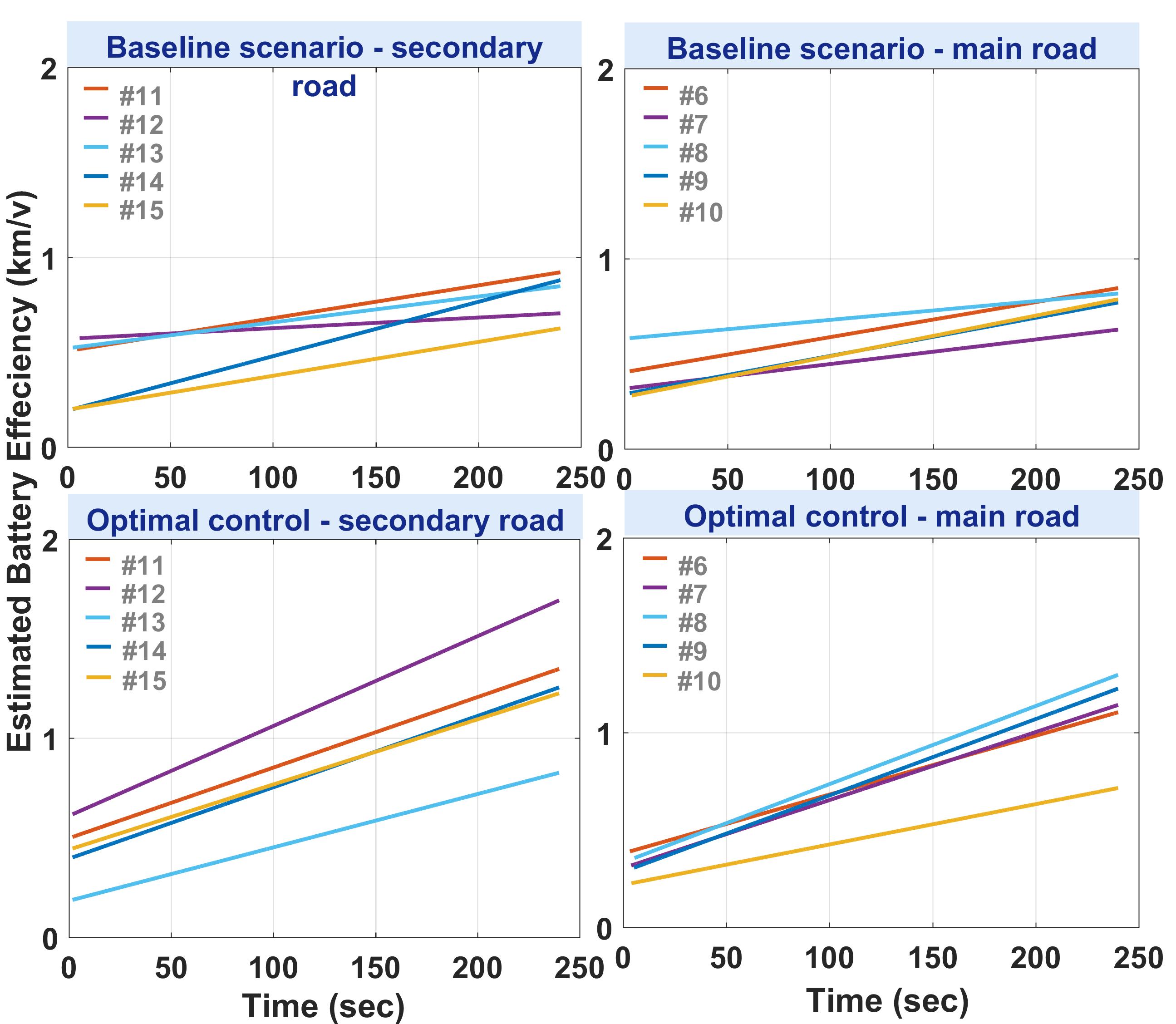
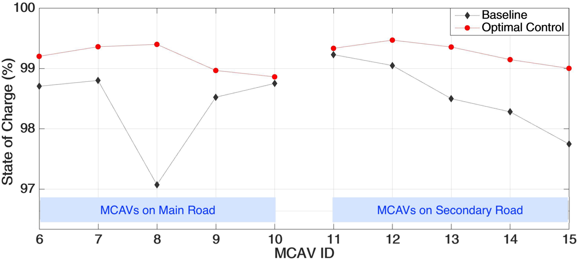
4.0.2 Battery State-of-Charge:
To quantify the benefits of vehicle coordination, we compare the battery State-of-Charge (SOC) for each MCAV. Under both scenarios, the MCAVs loop around the merging zone following a predefined trajectory. SOC is recorded for a 4-minute run. The estimated battery efficiencies for MCAVs under the two scenarios are illustrated in Fig. 6. From the final SOC of each MCAV (Fig. 7), it is clear that coordination of MCAVs improves the energy efficiency in the merging scenario due to the elimination of the stop-and-go driving.
5 Concluding Remarks
UDSSC is a small-scale “smart” city that can replicate real-world traffic scenarios in a small and controlled environment. This testbed can be an effective way to visualize the concepts developed in real world traffic scenarios using CAVs in a quick, safe, and affordable way. The UDSSC helps bridge the gap between theory and practical implementation by providing a means of simultaneously testing as many as 35 MCAVs. We used UDSSC to validate experimentally a control framework reported in Rios-Torres and Malikopoulos (2017b) for coordination CAVs. The results demonstrate that coordination of CAVs can improve the battery efficiency due to elimination of the stop-and-go driving. The integration of human driven MCAVs adds a promising direction for future work that may provide insights on the impact of CAVs in real world scenarios.
Caili Li (Univ. of Delaware) for assistance with software, Yue Feng (Univ. of Delaware) for WiFi communication and user interface, Grace Gong (Wilmington Charter High School) for MCAV design, and Abhinav Ratnagiri (Concord High School) for serial communication.
References
- Alonso et al. (2011) Alonso, J., Milanés, V., Pérez, J., Onieva, E., González, C., and de Pedro, T. (2011). Autonomous vehicle control systems for safe crossroads. Transportation Research Part C: Emerging Technologies, 19(6), 1095–1110.
- Antoniotti et al. (1997) Antoniotti, M., Deshpande, A., and Girault, A. (1997). Microsimulation analysis of automated vehicles on multiple merge junction highways. IEEE International Conference in Systems, Man, and Cybernetics, 839–844.
- Giuseppe and Vendittelli (2002) Giuseppe, Oriolo, D.L.A. and Vendittelli, M. (2002). Wmr control via dynamic feedback linearization: Design, implementation, and experimental validation. IEEE Transactions on Control Systems Technology, 10(6), 835–852.
- Kachroo and Li (1997) Kachroo, P. and Li, Z. (1997). Vehicle merging control design for an automated highway system. In Proceedings of Conference on Intelligent Transportation Systems, 224–229.
- Lu et al. (2000) Lu, X.Y., Tan, H.S., Shladover, S.E., and Hedrick, J.K. (2000). Implementation of longitudinal control algorithm for vehicle merging. Proceedings of the AVEC 2000.
- Malikopoulos and Aguilar (2013) Malikopoulos, A.A. and Aguilar, J.P. (2013). An Optimization Framework for Driver Feedback Systems. IEEE Transactions on Intelligent Transportation Systems, 14(2), 955–964.
- Malikopoulos et al. (2018) Malikopoulos, A.A., Cassandras, C.G., and Zhang, Y. (2018). A decentralized energy-optimal control framework for connected automated vehicles at signal-free intersections. Automatica.
- Margiotta and Snyder (2011) Margiotta, R. and Snyder, D. (2011). An agency guide on how to establish localized congestion mitigation programs. Technical report, U.S. Department of Transportation. Federal Highway Administration.
- Milanés et al. (2010) Milanés, V., Pérez, J., and Onieva, E. (2010). Controller for Urban Intersections Based on Wireless Communications and Fuzzy Logic. IEEE Transactions on Intelligent Transportation Systems, 11(1), 243–248.
- Ntousakis et al. (2016) Ntousakis, I.A., Nikolos, I.K., and Papageorgiou, M. (2016). Optimal vehicle trajectory planning in the context of cooperative merging on highways. Transportation Research Part C: Emerging Technologies, 71, 464–488.
- Ran et al. (1999) Ran, B., Leight, S., and Chang, B. (1999). A microscopic simulation model for merging control on a dedicated-lane automated highway system. Transportation Research Part C: Emerging Technologies, 7(6), 369–388.
- Rios-Torres et al. (2015) Rios-Torres, J., Malikopoulos, A.A., and Pisu, P. (2015). Online Optimal Control of Connected Vehicles for Efficient Traffic Flow at Merging Roads. In 2015 IEEE 18th International Conference on Intelligent Transportation Systems, 2432 – 2437.
- Rios-Torres and Malikopoulos (2017a) Rios-Torres, J. and Malikopoulos, A.A. (2017a). A Survey on Coordination of Connected and Automated Vehicles at Intersections and Merging at Highway On-Ramps. IEEE Transactions on Intelligent Transportation Systems, 18(5), 1066–1077.
- Rios-Torres and Malikopoulos (2017b) Rios-Torres, J. and Malikopoulos, A.A. (2017b). Automated and Cooperative Vehicle Merging at Highway On-Ramps. IEEE Transactions on Intelligent Transportation Systems, 18(4), 780–789.
- Schrank et al. (2015) Schrank, B., Eisele, B., Lomax, T., and Bak, J. (2015). 2015 Urban Mobility Scorecard. Technical report, Texas A& M Transportation Institute.
- Stager (2017) Stager, A. (2017). Information decision science (ids) lab presents the university of delaware scaled smart city. URL https://youtu.be/dVQmV98f-9M.
- VanMiddlesworth et al. (2008) VanMiddlesworth, M., Dresner, K., and Stone, P. (2008). Replacing the stop sign: unmanaged intersection control for autonomous vehicles. In Proc. 5th Workshop Agents Traffic Transport. Multiagent Syst., 94–101.
- Zhang et al. (2016) Zhang, Y., Malikopoulos, A.A., and Cassandras, C.G. (2016). Optimal control and coordination of connected and automated vehicles at urban traffic intersections. In Proceedings of the 2016 American Control Conference, 5014–5019.