Local Gyrokinetic Study of Electrostatic Microinstabilities in Dipole Plasmas

Abstract

A linear gyrokinetic particle-in-cell scheme, which is valid for arbitrary perpendicular wavelength $k_{\perp}\rho_{i}$ and includes the parallel dynamic along the field line, is developed to study the local electrostatic drift modes in point and ring dipole plasmas. We find the most unstable mode in this system can be either electron mode or ion mode. The properties and relations of these modes are studied in detail as a function of $k_{\perp}\rho_{i}$, the density gradient $\kappa_{n}$, the temperature gradient $\kappa_{T}$, electron to ion temperature ratio $\tau=T_{e}/T_{i}$, and mass ratio $m_{i}/m_{e}$. For conventional weak gradient parameters, the mode is on ground state (with eigenstate number $l=0$) and especially $k_{\parallel}\sim 0$ for small $k_{\perp}\rho_{i}$. Thus, bounce averaged dispersion relation is also derived for comparison. For strong gradient and large $k_{\perp}\rho_{i}$, most interestingly, higher order eigenstate modes with even (e.g., $l=2,4$) or odd (e.g., $l=1$) parity can be most unstable, which is not expected by previous studies. High order eigenstate can also easily be most unstable at weak gradient when $\tau>10$. This work can be particularly important to understand the turbulent transport in laboratory and space magnetosphere.

I Introduction

Dipole magnetic fields widely exist in the Universe, such as in the planetary magnetospheres. The idea of using strong dipole field configuration for magnetic confinement of laboratory plasmas for fusion is proposed theoretically by Hasegawa Hasegawa1987 ; Hasegawa1990 and several experimental devices have also been built since then, such as the Levitated Dipole Experiment (LDX) Boxer2008 ; Boxer2010 ; Garnier2017 at MIT, the Collisionless Terrella Experiment (CTX) Levitt2002 at Columbia University and Ring Trap-1 (RT-1) Yoshida2006 ; Yoshida2013 at the University of Tokyo. The dipole configuration is also used to confine electron-positron pair plasmas in the laboratorySarri2015 . Typical charged particle trajectories under ideal dipole field have good confinement features. The collision and electrostatic or electromagnetic turbulence can break this ideal confinement. Previous theoretical and experimental results in Refs.Boxer2008 ; Boxer2010 ; Garnier2017 show that the dipole confinement is good even under the stochastic motion of particles due to the collision and turbulence, at least under the present laboratory low temperature and density parameters. However, the confinement properties of dipole field under fusion parameters, e.g., high temperature and density and the gradient of them, are still open questions.

In this work, we develop a local gyrokinetic particle code to understand the linear behaviors of electrostatic microinstabilities in point (ideal) and ring dipole plasmas. In contrast to previous studiesKesner1998 ; Kesner2000 ; Kesner2002 ; Simakov2001 ; Helander2016 , we do not limit our study to small $k_{\perp}\rho_{i}$, where $k_{\perp}$ is the perpendicular wavevector and $\rho_{i}$ is the ion Lamor radius. Comprehensive investigations of the linear features of the electrostatic drift modes can be important to understand the nonlinear physicsHorton1999 , such as the simulation results of the typical electrostatic turbulent transport features in ring dipole configuration in Refs.Kobayashi2009 ; Kobayashi2010 . Several electromagnetic studies Simakov2002 ; Dettrick2003 ; Porazik2011 ; Mager2017 of the Alfvénic drift modes in dipole configuration also exist, which is not the aim of the present work. We also noticed that Ref.Zhao2001 had attempted to build a particle-in-cell model similar to our present work using gyrokinetic ion but bounce-averaged electron model in local point dipole configuration.

In the following sections, we provide a comprehensive derivations of our model. Sec.II gives the linearized gyrokinetic model equations. Sec.III provides the details of the dipole coordinate system and operators. Sec.IV gives the relevant zero-dimensional dispersion relation. Sec.V discusses some details of our particle-in-cell model. Sec.VI benchmarks our simulation model. Sec.VII shows the details of our simulation results. Sec.VIII summarizes the present study.

II Linear Gyrokinetic Model

We use standard linear gyrokinetic modelAntonsen1980 ; Chen1991 , which can describe the low frequency physics accurately under the assumptions: $\omega/\Omega_{ci}\sim\rho_{i}/L\sim k_{\parallel}/k_{\perp}\ll 1$. Assuming Maxwellian equilibrium distribution function $F_{0}=n_{0}F_{M}$, with $F_{M}=(\frac{m}{2\pi T})^{3/2}e^{-m\epsilon/T}$, $\epsilon=v^{2}/2$, $\mu=v_{\perp}^{2}/2B$, the perturbation distribution function after gyrophase average is

$$f_{s}=\frac{q_{s}}{m_{s}}\frac{\partial F^{s}_{0}}{\partial\epsilon}\phi+J_{0}(k_{\perp}\rho_{s})h_{s}.$$ (1)

The non-adiabatic gyrokinetic response $h_{s}$ satisfies

$$(\omega-\omega_{Ds}+iv_{\parallel}{\bf b}\cdot{\bf\nabla})h_{s}=-(\omega-\omega_{*s}^{T})\frac{\partial F^{s}_{0}}{\partial\epsilon}\frac{q_{s}}{m_{s}}J_{0}\phi,$$ (2)

where the first kind Bessel function $J_{0}$ comes from gyrophase average, and the parameters are

$$\rho_{s} = \frac{v_{\perp}}{\Omega_{s}},~{}~{}~{}~{}\Omega_{s}=\frac{q_{s}B}{m_{s}c},$$

$$\frac{\partial F^{s}_{0}}{\partial\epsilon} = -\frac{m_{s}F_{0}^{s}}{T_{s}},~{}~{}~{}{\bf b}={\bf B}/B,$$

$$\omega_{*s}^{T} = \frac{{\bf k}_{\perp}\times{\bf b}\cdot{\bf\nabla}F^{s}_{0}}{-\Omega_{s}F^{s}_{0\epsilon}},$$

$$\omega_{Ds} = {\bf k}_{\perp}\cdot{\bf v}_{d}={\bf k}_{\perp}\cdot{\bf b}\times\frac{\mu\nabla B+v_{\parallel}^{2}{\bf b}\cdot\nabla{\bf b}}{\Omega_{s}}.$$

Here, $s=i,e$ represents particle species, and the collision term is neglected. ${\bf B}$ is the magnetic field, and $q_{s}$, $m_{s}$, $T_{s}$, $\Omega_{s}$, $\rho_{s}$, $\omega_{*s}^{T}$ and $\omega_{Ds}$ are the charge, mass, temperature, cyclotron frequency, gyroradius, diamagnetic drift frequency and magnetic (gradient and curvature) drift frequency for the species $s$, respectively.

In electrostatic case, the gyrokinetic system is closed by quasi-neutrality condition (Poisson equation)

$$\sum_{\alpha}q_{\alpha}\int f_{\alpha}d^{3}v=0,$$ (3)

where the notation for velocity integral $\int d^{3}v\equiv 2\pi\int\frac{B}{|v_{\parallel}|}d\epsilon d\lambda$, with pitch angle variable $\lambda\equiv\mu B_{0}/\epsilon$. In Eq.(3), we have assumed the Debye length is far smaller than the ion gyroradius, i.e., $\lambda_{D}\ll\rho_{i}$. For the present work, we focus on the one-dimensional (1D) physics along the field line and thus ${\bf b}\cdot{\bf\nabla}=\partial_{l}$.

For initial value approach, we can define

$$g_{s}\equiv h_{s}-\frac{q_{s}}{T_{s}}F^{s}_{0}J_{0}\phi,~{}{\rm i.e.},~{}f_{s}=-\frac{q_{s}}{T_{s}}F^{s}_{0}(1-J_{0}^{2})\phi+J_{0}g_{s},$$ (4)

and Eq.(2) changes to (with also $\omega=i\partial_{t}$)

$$(\partial_{t}+v_{\parallel}\partial_{l})g_{s} = -i\omega_{Ds}g_{s}-i(\omega_{Ds}-\omega_{*s}^{T})\frac{q_{s}}{T_{s}}F^{s}_{0}J_{0}\phi$$ (5)

$$-v_{\parallel}\frac{q_{s}}{T_{s}}F^{s}_{0}[J_{0}\partial_{l}\phi-J_{1}\partial_{l}(k_{\perp}\rho_{s})\phi],$$

where we have used $J^{\prime}_{0}=-J_{1}$. For only one species of ion, i.e., $s=i,e$ and $q_{i}=-q_{e}=e$, Eq. (3) can be rewritten as

$$-\frac{q_{i}n_{i}}{T_{i}}(1-\Gamma_{0i})\phi+\int J_{0i}g_{i}d^{3}v=$$

$$-\frac{q_{e}n_{e}}{T_{e}}(1-\Gamma_{0e})\phi+\int J_{0e}g_{e}d^{3}v,$$ (6)

where $\Gamma_{0s}\equiv I_{0}(b_{s})e^{-b_{s}}$, with $I_{0}$ the modified Bessel function, $b_{s}=\Big{(}\frac{k_{\perp}v_{ts}}{\Omega_{s}}\Big{)}^{2}$ and $v_{ts}=\sqrt{T_{s}/m_{s}}$. We have solved the above gyrokinetic system Eqs.(5) and (II) in Z-pinch with only passing particles using MGK code in Ref.Xie2017a , where we can assume $v_{\parallel}$ and $v_{\perp}$ to be constant along field line. However, to study the physics in dipole configuration, we must treat the particles trapping, i.e., the variation of $v_{\parallel}$ and $v_{\perp}$ along the field line.

III Dipole Equilibrium Operators

For idea point dipole or current loop ring dipole, the equilibrium magnetic field ${\bf B}$ is symmetric in toroidal direction, thus we can write

$${\bf B} = \nabla\zeta\times\nabla\psi=\nabla\chi,$$

$${\bf k}_{\perp} = k_{\psi}\nabla\psi+k_{\zeta}\nabla\zeta,$$

where $\zeta$ is azimuthal (toroidal) angle, and $\psi$ is flux surface function (radial). The above equilibrium can be a good equilibrium model for plasma at low $\beta$, where $\beta$ is the ratio of plasma pressure and magnetic pressure.

In this section, we summarize the derivations of the operators in our simulation model for ring dipole configuration and leave the detailed derivations using point dipole as example in the Appendix B. We firstly define torus coordinates $(r,\theta,\phi)$ with $R=a+r\cos\theta$, and flux coordinates $(\psi,\chi,\zeta)$ with $\psi=\psi(r,\theta)$, $\chi=\chi(r,\theta)$ and $\zeta=\phi$. And we define $\xi=\theta\in[-\pi,\pi]$, along the field line

$$dl=r_{0}\kappa(\xi)d\xi,$$ (7)

where we take $r_{0}=\frac{R(\theta=0)-R(\theta=\pi)}{2}$, and we have

$$\frac{\partial}{\partial l}=\frac{\partial}{\partial\xi}\frac{\partial\xi}{\partial l}=\frac{1}{r_{0}\kappa}\frac{\partial}{\partial\xi}.$$ (8)

For point dipole, $\kappa=\cos\xi(1+3\sin^{2}\xi)^{1/2}$, $\xi=\pi/2-\theta$ and $\theta$ is spherical coordinate. For Z-pinch, $\kappa=1$. Considering $\epsilon$ and $\mu$ conserved, pitch angle $\lambda\equiv\mu B_{0}/\epsilon$, $v_{\parallel}=\sqrt{2(\epsilon-\mu B)}=v\sqrt{1-\lambda B/B_{0}}$, $v=\sqrt{2\epsilon}$, $v^{2}=v_{\parallel}^{2}+v_{\perp}^{2}$, $B=B_{0}f(\xi)$ and $v_{\parallel}=dl/dt$, we have

$$\frac{d\xi}{dt}=\frac{v_{\parallel}}{r_{0}\kappa}=\frac{\pm v\sqrt{y}}{r_{0}\kappa},$$ (9)

with $y=1-f(\xi)\lambda$. For point dipole, $f(\xi)=\frac{\sqrt{1+3\sin^{2}\xi}}{\cos^{6}\xi}$. For Z-pinch, $f=1$.

Taking ${\bf k}_{\perp}=k_{\psi}\nabla\psi+k_{\zeta}\nabla\zeta$, $k_{\perp}=|{\bf k}_{\perp}|$, $k_{\psi}=0$ for ring dipole, and using ${\bf B}=\nabla\zeta\times\nabla\psi=\nabla\chi$ and $\nabla\zeta=\frac{1}{R}{\bm{\hat{}}e}_{\phi}$, we obtain along a field line

$$k_{\perp}^{2}=k_{\zeta}^{2}\nabla\zeta\cdot\nabla\zeta=k_{\zeta}^{2}\frac{1}{r_{0}^{2}p_{0}^{2}p^{2}}=k_{t}^{2}\frac{1}{r_{0}^{2}p^{2}},$$

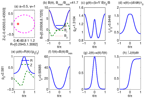
Figure 1: Configuration functions along a field line in ring dipole case.

where we have taken $R=r_{0}p_{0}p(\xi)$, i.e., $p(\xi)\equiv R/(r_{0}p_{0})$, and $k_{t}\equiv k_{\zeta}/p_{0}$. We introduce a constant $p_{0}$ to make the configuration function $p(\xi=0)=1$, and hence the notations can be convenient for different configurations. An example of $p(\xi)$ for ring dipole is shown in Fig.1(e), where $R$ and $Z$ are the cylindrical coordinate $(R,\zeta,Z)$ normalized by $R(\theta=0)$. For Z-pinch, we have $p_{0}=a/r_{0}$ and $p=1$. We can also readily obtain $\rho_{s}=\frac{v_{\perp}}{\Omega_{s}}=\frac{\sqrt{2\mu B}}{q_{s}B/m_{s}c}=\frac{\sqrt{2\mu B_{0}}}{\Omega_{s0}}\sqrt{\frac{B_{0}}{B}}=\frac{v\sqrt{\lambda}}{\Omega_{s0}}\frac{1}{\sqrt{f(\xi)}}$. Thus $k_{\perp}\rho_{s}=k_{t}\frac{v\sqrt{\lambda}}{r_{0}\Omega_{s0}}\frac{1}{z}$, with $z(\xi)=p(\xi)\sqrt{f(\xi)}$, and $\partial_{\xi}(k_{\perp}\rho_{s})=k_{t}\frac{v\sqrt{\lambda}}{r_{0}\Omega_{s0}}\partial_{\xi}(z^{-1})=-k_{t}\frac{v\sqrt{\lambda}}{r_{0}\Omega_{s0}}z^{-2}\partial_{\xi}z$, and $b_{s}=\Big{(}\frac{k_{\perp}v_{ts}}{\Omega_{s}}\Big{)}^{2}=\frac{k_{t}^{2}v_{ts}^{2}}{r_{0}^{2}\Omega_{s0}^{2}}\frac{1}{p^{2}f^{2}}$.

Since $n_{0}=n_{0}(\psi)$ and $T_{0}=T_{0}(\psi)$, we can have

$$\nabla F_{0} = \nabla\Big{[}n_{0}(\frac{m}{2\pi T_{0}})^{3/2}e^{-m\epsilon/T_{0}}\Big{]}$$

$$= \Big{\{}\frac{\nabla n_{0}}{n_{0}}+\frac{\nabla T_{0}}{T_{0}}\Big{[}\frac{m\epsilon}{T_{0}}-\frac{3}{2}\Big{]}\Big{\}}F_{0}$$

$$= -\nabla\psi\Big{\{}L_{n}^{-1}+L_{T}^{-1}\Big{[}\frac{m\epsilon}{T_{0}}-\frac{3}{2}\Big{]}\Big{\}}F_{0}$$

$$= \frac{\nabla n_{0}}{n_{0}}\Big{\{}1+\eta_{s}\Big{[}\frac{m\epsilon}{T_{0}}-\frac{3}{2}\Big{]}\Big{\}}F_{0},$$

where $T_{s}=m_{s}v_{ts}^{2}$, $L_{n}^{-1}\equiv-\frac{\partial\ln n_{0}}{\partial\psi}$, $L_{T}^{-1}\equiv-\frac{\partial\ln T_{0}}{\partial\psi}$ and $\eta_{s}=\frac{L_{n}}{L_{T_{s}}}$. And by further using

$$({\bf k_{\perp}}\times{\bf b})\cdot\nabla n_{0} = \frac{1}{B}[(k_{\psi}\nabla\psi+k_{\zeta}\nabla\zeta)\times\nabla\chi]\cdot\nabla\psi\frac{\partial n_{0}}{\partial\psi}$$

$$= \frac{1}{B}[k_{\zeta}\nabla\zeta\times\nabla\chi]\cdot\nabla\psi\frac{\partial n_{0}}{\partial\psi}$$

$$= k_{\zeta}B\frac{\partial n_{0}}{\partial\psi},$$

we obtain

$$\omega_{*s}^{T} = \frac{{\bf k}_{\perp}\times{\bf b}\cdot{\bf\nabla}F^{s}_{0}}{-\Omega_{s}F^{s}_{0\epsilon}}=\frac{{\bf k}_{\perp}\times{\bf b}\cdot{\bf\nabla}F^{s}_{0}}{m_{s}\Omega_{s}F^{s}_{0}/T_{s}}$$

$$= \frac{k_{\zeta}B\frac{\partial n_{0}}{\partial\psi}\frac{1}{n_{0}}\Big{\{}1+\eta_{s}\Big{[}\frac{m\epsilon}{T_{0}}-\frac{3}{2}\Big{]}\Big{\}}}{m_{s}\Omega_{s}/T_{s}}$$

$$= -\omega_{*s}\Big{\{}1+\eta_{s}\Big{[}\frac{m\epsilon}{T_{0}}-\frac{3}{2}\Big{]}\Big{\}},$$

where $\omega_{*s}=\frac{k_{\zeta}cT_{s}}{q_{s}L_{ns}}$.

The gradient drift ${\bm{v}}_{g}$, curvature drift ${\bm{v}}_{c}$, and total drift ${\bm{v}}_{d}={\bm{v}}_{g}+{\bm{v}}_{c}$ are

$${\bm{v}}_{g}=\frac{1}{m\Omega_{s}}\mu{\bm{b}}\times\nabla B=-\frac{v_{\perp}^{2}}{2\Omega_{s}B}({\bm{b}}\times\nabla B){{\hat{e}}_{\phi}},$$ (10)

$${\bm{v}}_{c}=\frac{1}{\Omega_{s}}v_{\parallel}^{2}\nabla\times{\bm{b}}=-\frac{v_{\parallel}^{2}}{\Omega_{s}B}({\bm{b}}\times\nabla B){{\hat{e}}_{\phi}},$$ (11)

$${\bm{v}}_{d}=-\frac{{\bm{b}}\times\nabla B}{B\Omega_{s}}(v_{\parallel}^{2}+\frac{1}{2}v_{\perp}^{2}){{\hat{e}}_{\phi}}=-\frac{g}{r_{0}\Omega_{s0}f}(v_{\parallel}^{2}+\frac{1}{2}v_{\perp}^{2}){{\hat{e}}_{\phi}},$$ (12)

where we have defined $({\bm{b}}\times\nabla B)/B=g(\theta)/r_{0}$, which would be calculated numerically. Note that $\nabla\times{\bm{b}}=\nabla\times\frac{\bm{B}}{B}=\frac{1}{B}\nabla\times{\bm{B}}+\Big{(}\nabla\frac{1}{B}\Big{)}\times{\bm{B}}=\frac{{\bm{b}}}{B}\times\nabla B$, where we have used $\nabla\times{\bm{B}}=0$ for vacuum field. And thus we obtain

$$\omega_{Ds}={\bf k_{\perp}}\cdot{\bm{v}}_{d}=\frac{-k_{t}g}{r_{0}^{2}\Omega_{s0}fp}(v_{\parallel}^{2}+\frac{1}{2}v_{\perp}^{2})=\frac{-\omega_{d0}g}{fp}\frac{(1+y)}{2}v^{2},$$ (13)

where $\omega_{d0}=\frac{k_{t}}{r_{0}^{2}\Omega_{s0}}$. For point dipole, $g(\theta)=\frac{3(\cos^{2}\theta+1)}{\sin\theta(1+3\cos^{2}\theta)^{3/2}}$, $r=r_{0}\sin^{2}\theta$. For Z-pinch, $g=1$.

For a typical ring dipole parameter, the corresponding $B$, $f$, $\kappa$, $g$ and $p$ on $\theta$ are shown in Fig.1, where the $\bm{B}$ field is calculated using the elliptic functions based on Appendix A. This typical ring dipole configuration will be used in later simulations in Sec.VII.

Treating electron and ion using the same kinetic equation, with $q_{i}=-q_{e}=e$, $n_{i0}=n_{e0}$, $\tau_{e}=T_{e}/T_{i}$, and defining the $\delta f$ weight $w=g/F_{0}$, the kinetic equation Eq.(5) can be rewritten as

$$\frac{d\xi_{s}}{dt}=\frac{v_{\parallel}}{r_{0}\kappa},$$ (14)

$$\frac{dw_{s}}{dt} = -i\omega_{Ds}w_{s}-i(\omega_{Ds}-\omega_{*s}^{T})\frac{q_{s}}{T_{s}}J_{0}\phi$$

$$-v_{\parallel}\frac{q_{s}}{T_{s}}\frac{1}{r_{0}\kappa}[J_{0}\partial_{\xi}\phi-J_{1}\partial_{\xi}(k_{\perp}\rho_{s})\phi],$$

and the quasi-neutrality Eq. (II) does not change.

Considering $\tau=\tau_{e}=T_{e}/T_{i}$, $v_{te}=v_{ti}\sqrt{\tau m_{i}/m_{e}}$, $\Omega_{e}=\frac{q_{e}m_{i}}{q_{i}m_{e}}\Omega_{i}$, $\rho_{te}=\rho_{ti}\frac{q_{i}}{q_{e}}\sqrt{\tau\frac{m_{e}}{m_{i}}}$, and defining $k_{s}\equiv k_{\perp}\rho_{ts}$, we normalize the equations by $v_{0}$ and $R_{0}$. We assume hot ion, and take $v_{0}=v_{ti}$, $R_{0}=r_{0}$. Thus, we have: length $L\to L/r_{0}$, velocity $v\to v/v_{0}$, time $t_{0}=r_{0}/v_{0}$, $t\to t/t_{0}$, frequency $\omega_{0}=v_{0}/r_{0}$, $\rho_{ti}=v_{0}/\Omega_{0i}$, $\epsilon_{n}\equiv-\frac{1}{B_{0}p_{0}r_{0}^{2}}\Big{(}\frac{\partial\ln n_{0}}{\partial\psi}\Big{)}^{-1}=L_{n}/(B_{0}p_{0}r_{0}^{2})$, $\phi\to e\phi/T_{i}$. The normalized variables are $\rho_{ti}\to\rho_{ti}/r_{0}=\omega_{0}/\Omega_{0i}$, $\rho_{te}=\rho_{ti}\frac{q_{i}}{q_{e}}\sqrt{\tau\frac{m_{e}}{m_{i}}}$, $F_{0s}=(\frac{1}{2\pi v_{ts}^{2}})^{3/2}e^{-v^{2}/2v_{ts}^{2}}$, $v_{ti}\to 1$, $v_{te}\to\sqrt{\tau m_{i}/m_{e}}$, and wavevectors $k_{\perp}\to k_{\perp}r_{0}$, $k_{\zeta}\to k_{\zeta}$, $k_{\psi}\to k_{\psi}B_{0}r_{0}^{2}$. And hence

$$k_{\perp}^{2}=k_{t}^{2}/p^{2},~{}~{}~{}k_{\perp}\rho_{s}=\frac{v}{v_{ts}}\sqrt{\lambda}k_{t}\rho_{ts}z^{-1},$$

$$\partial_{\xi}(k_{\perp}\rho_{s})=-\frac{v}{v_{ts}}\sqrt{\lambda}k_{t}\rho_{ts}z^{-2}\partial_{\xi}z,~{}~{}~{}b_{s}=\rho_{ts}^{2}k_{t}^{2}\frac{1}{p^{2}f^{2}}.$$

Normalized diamagnetic drift frequency is

$$\omega_{*s}^{T}=-\omega_{*s}\Big{\{}1+\eta_{s}\Big{[}\frac{v^{2}}{2v_{ts}^{2}}-\frac{3}{2}\Big{]}\Big{\}}=-\omega_{s0}\Big{\{}\kappa_{n}+\kappa_{T}\Big{[}\frac{v^{2}}{2v_{ts}^{2}}-\frac{3}{2}\Big{]}\Big{\}},$$

where $\omega_{*i}=k_{t}\omega_{0}\rho_{ti}/\epsilon_{n}\to k_{t}\rho_{ti}/\epsilon_{n}$, $\omega_{*e}=\frac{q_{i}}{q_{e}}\tau\omega_{*i}$, $\kappa_{n}=\epsilon_{n}^{-1}$ and $\kappa_{T}=\eta_{s}\epsilon_{n}^{-1}$. Normalized curvature drift frequency is

$$\omega_{Ds}=-\omega_{ds0}\frac{g}{fp}\frac{(1+y)}{2}\frac{v^{2}}{v_{ts}^{2}},$$

where $\omega_{di0}=k_{t}\omega_{0}\rho_{ti}\to k_{t}\rho_{ti}$ and $\omega_{de0}=\tau\frac{q_{i}}{q_{e}}\omega_{di0}$.

The final gyrokinetic system changes to

$$\frac{d\xi_{s}}{dt}=\frac{v_{\parallel}}{\kappa},$$ (16)

$$\frac{dw_{s}}{dt} = -i\omega_{Ds}w_{s}-i(\omega_{Ds}-\omega_{*s}^{T})\frac{q_{s}}{T_{s}}J_{0}\phi$$

$$-v_{\parallel}\frac{1}{\kappa}\frac{q_{s}}{T_{s}}[J_{0}\partial_{\xi}\phi-J_{1}\partial_{\xi}(k_{\perp}\rho_{s})\phi],$$

$$\Big{(}1+\frac{1}{\tau_{e}}-\Gamma_{0i}-\frac{1}{\tau_{e}}\Gamma_{0e}\Big{)}\phi=\int J_{0i}g_{i}d^{3}v-\int J_{0e}g_{e}d^{3}v.$$ (18)

To avoid the sign change of $v_{\parallel}$ at the turning point, we add an extra equation to calculate $v_{\parallel}$

$$\frac{dv_{\parallel}}{dt}=-\frac{v^{2}\lambda}{2r_{0}}\frac{1}{\kappa}\frac{df}{d\xi}\to-\frac{v^{2}\lambda}{2}\frac{1}{\kappa}\frac{df}{d\xi},$$ (19)

which can be derived from Eq.(9) via $\mu$ and $\epsilon$ conservation. For point dipole, $\frac{dv_{\parallel}}{dt}=-\frac{v^{2}\lambda}{2}\frac{3\sin\xi(3+5\sin^{2}\xi)}{\cos^{8}\xi(1+3\sin^{2}\xi)}$, which can also be derived via mirror force $F=-\mu\nabla B$, i.e., $F_{\parallel}=-\mu(\partial_{\chi}B)|{\bm{e}}^{\chi}|$. Eqs.(16)-(19) are our final equations to solve for local electrostatic drift mode in dipole. Standard $\delta f$ particle-in-cell (PIC) approach Parker1993 ; Xie2017a is used in this work to do our simulation. If we use adiabatic electron model, i.e., $h_{e}=0$ (not $g_{e}=0$), the only change is the quasi-neutrality Eq.(18), which should be changed to

$$\Big{(}1+\frac{1}{\tau_{e}}-\Gamma_{0i}\Big{)}\phi=\int J_{0i}g_{i}d^{3}v.$$ (20)

In the latter part, we will check whether the adiabatic electron model is valid for dipole simulations.

One should also note the slight difference of the definitions of our notations between ring dipole and point dipole. These differences mainly come from the coordinate system: for ring dipole we calculate our variables from torus coordinate; whereas for point dipole we calculate them from spherical coordinate. Thus, for examples, if we reduce $a\to 0$ in ring dipole case, we obtain the curvature radius at $\xi=0$ to be $R_{c}^{\rm ring-dipole}=2R/3$, which is not $R_{c}^{\rm point-dipole}=R/3$ as in the point dipole case. And for Z-pinch $R_{c}^{\rm Z-pinch}=R$. That is, if we want to quantitatively compare the results in ring dipole and point dipole, we should keep in mind the normalization $R$ is $R^{\rm point}\sim 2R^{\rm ring}$. This difference will affect $\kappa_{n}$, $\kappa_{T}$, $\omega_{D}$ and so on. In our normalization in this work, $\omega_{*i}<0$ and $\omega_{*e}>0$, and thus positive real frequency means the mode propagates in electron diamagnetic direction and negative real frequency means the mode propagates in the ion diamagnetic direction.

IV Zero-dimensional Dispersion relation

In ideal dipole field, all particles are trapped particles and the simplest dispersion relation is replacing $\omega_{D}$ by bounce average $\langle\omega_{D}\rangle_{b}$, and setting $\langle J_{0}(k_{\perp}\rho)\phi\rangle_{b}=\langle J_{0}(k_{\perp}\rho)\rangle_{b}\phi$ by assuming $k_{\parallel}=0$. We have

$$\sum_{s=e,i}\int dv^{3}[1-\omega_{*}^{T}(v)/\omega]\partial_{\epsilon}F(v)\Big{\{}\phi-\frac{J_{0}\oint J_{0}\phi dl/v_{\parallel}}{\oint[1-\omega_{D}(v)/\omega]dl/v_{\parallel}}\Big{\}}=0,$$ (21)

where $F(v)$ is Maxwellian isotropic equilibrium distribution function. This yields the normalized final dispersion relation

$$D(\omega,k)=\sum_{s=e,i}\frac{1}{T_{s}}\Big{\{}1-\int dv^{3}\frac{[\omega-\omega_{*}^{T}(v)]J_{0}\langle J_{0}\rangle_{b}}{[\omega-k_{zs}v_{\parallel}-\langle\omega_{D}(v)\rangle_{b}]}e^{-\frac{v^{2}}{2}}\Big{\}}=0.$$ (22)

where $\int dv^{3}=\frac{1}{\sqrt{2\pi}}\int_{-\infty}^{\infty}dv_{\parallel}\int_{0}^{\infty}v_{\perp}dv_{\perp}$, and we have artificially added back the $k_{\parallel}$ term to make it more general, with $k_{zi}=k_{\parallel}R$ and $k_{ze}=k_{\parallel}R\sqrt{\tau m_{i}/m_{e}}$. Eq.(22) can be seen as an extension of the one in Refs.Rutherford1968 ; Kesner1998 . The above dispersion relation Eq.(22) is similar to the one in Z-pinchRicci2006 ; Xie2017a , except several bounce average terms. The bounce average $\langle\omega_{D}\rangle_{b}$ and $\langle J_{0}\rangle_{b}$ can be found at Appendix C. Interpolation or fitting can be used to speed up the numerical calculation. The details of the root finding method can be found at Ref.Xie2017a . One should also note that it is not easy to do the bounce average accurately especially when considering $k_{\perp}\rho_{i}$ not small in $J_{0}$. Refs.Kesner2002 ; Helander2016 only discussed the $J_{0}\to 1$ limit. As will be shown in Fig.4, if we modify the term $J_{0}\langle J_{0}\rangle_{b}$ to $J_{0}^{2}$, $\langle J_{0}\rangle_{b}^{2}$ or $\langle J_{0}^{2}\rangle_{b}$, the solutions will change quantitatively but not qualitatively, i.e., the essential physics is the same.

V Particle-in-cell approach

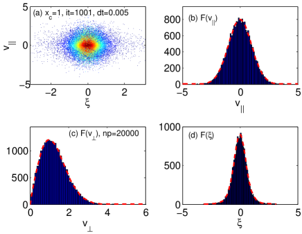
Figure 2: After $nt=1000$ time steps, the distribution function $F(\theta,v_{\parallel},v_{\perp},t)$ (the bar charts) still agrees with the initial loading $F_{0}=F(\theta,v_{\parallel},v_{\perp},t=0)$ (the red dash line) in ring dipole case.

The main steps of $\delta f$ particle-in-cell model Parker1993 used here are summarized in Ref.Xie2017a . However, in this work we should carefully treat the non-uniform magnetic field, which strongly affects the particle loading to keep the equilibrium distribution function $F_{0}$ constant with time, i.e., $\partial F_{0}/\partial t=0$. In our simulation model, we load the velocity using Gaussian random number as in Ref.Xie2017a , i.e., Maxwellian $v_{\parallel}=randn(np)\times v_{t}$ and $v_{\perp}=\sqrt{randn(np)^{2}+randn(np)^{2}}\times v_{t}$. Here, $n_{p}$ is particle number for one species, $j=1,2,\cdots,n_{p}$ is particle index, and $randn()$ generates normal distribution $F_{0}=\frac{1}{\sqrt{2\pi}}e^{-x^{2}/2}$. The initial spatial position $\xi_{j}$ should be loaded according to the flux-tube volume, i.e., $F_{0}(\xi)\propto J(\theta)=\kappa(\theta)/f(\theta)$, where $J(\theta)$ can be seen as Jacobian metric. For point dipole, $J(\xi)=\cos^{7}\xi$. We use acceptance-rejection method to generate this nonuniform loading of $\xi_{j}$. We note that the particle loading approaches in Refs.Dettrick2003 ; Bierwage2008 are different, which are more complicated. We have verified our approach that the equilibrium distribution function indeed remains unchanged with time, as shown in Fig.2.

We use periodic boundary condition for field, i.e., $\phi(n_{g}+1)=\phi(1)$, where $n_{g}$ is the field grid number for spatial coordinate $\xi$. The particles are also treated periodically, i.e., if a particle passes one boundary, we let it enter the simulation domain at another boundary. The simulation box is $\xi/\pi\to[-x_{c},x_{c}]$. That is, we do not need to simulate the whole field line. If we set $x_{c}\to 0$, the simulation results should reduce to the slab case and should agree with the dispersion relation accurately. By varying $x_{c}$ we examine how the results change from Z-pinch configuration to dipole configuration, i.e., $x_{c}\to 0$ for Z-pinch case and $x_{c}=1$ (or $x_{c}\to 0.5$) for ring (or point) dipole case.

One difficulty of the present simulation model is to study the $k_{\perp}\rho_{i}\ll 1$ modes at large $B$ field region, due to the term $G_{\rm coef}=\Big{(}1+\frac{1}{\tau_{e}}-\Gamma_{0i}-\frac{1}{\tau_{e}}\Gamma_{0e}\Big{)}\simeq b_{i}^{2}\to 0$ in the field equation, especially for $\xi$ around the simulation edge ($|\xi|\to\pi/2$). We take point dipole for example: The magnetic field at $\xi_{c}$ is $f(\xi_{c})$; The ratio of particles at $|\xi|>\xi_{c}$ is $N_{\rm ratio}=1-\int_{-\xi_{c}}^{\xi_{c}}J(\xi)d\xi/\int_{-\pi/2}^{\pi/2}J(\xi)d\xi$. Some typical values are listed in Table.1. We can see that only $N_{\rm ratio}\sim 10^{-5}$ particles exist at $|\xi|>0.4\pi$ which is difficult to represent the density integral $\int J_{0i}g_{i}d^{3}v$ accurately and the coefficient $G_{\rm coef}\sim 10^{-4}$ is very small if we take $k_{\perp}\rho_{i}\sim 1$. Thus, the electrostatic potential $\phi$ calculated from the quasi-neutrality Eq.(18) will have large numerical error at larger $|\xi|$. At this stage, we have not fully resolved this difficulty but use large particle number $n_{p}$ and adjust $x_{c}$ to overcome it.

Table 1: Numerical difficulty for small $k_{\perp}\rho_{i}$ due to the strong magnetic at edge ($|\xi|\to\pi/2$) in point dipole.

$\xi_{c}/\pi$	$B/B_{0}$	$b_{i}^{2}$	$N_{\rm ratio}$
0	1	1	1
0.05	1.116	0.8649	0.6661
0.1	1.533	0.5752	0.3850
0.15	2.542	0.3092	0.1875
0.2	5.090	0.1377	0.07394
0.25	12.65	0.05	0.0222
0.3	41.74	0.0139	4.59e-3
0.35	210.0	2.59e-3	5.40e-4
0.4	2.21e4	2.35e-4	2.37e-5
0.45	1.35e5	3.73e-6	9.90e-8
0.5	$\infty$	0	0

VI Benchmark and basic features of the modes

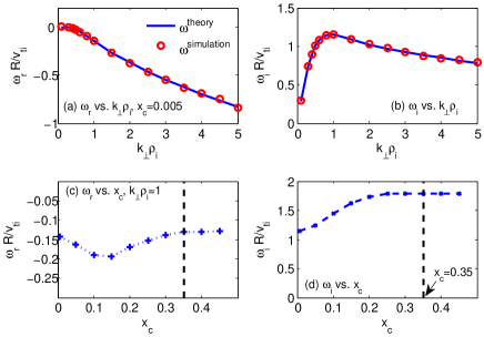
Figure 3: Benchmark of the simulation model in point dipole configuration: (a&b) Scanning $\omega$ vs. $k_{\perp}\rho_{i}$ with $x_{c}=0.005$, and comparing with the slab dispersion relation solution; (c&d) Scanning $\omega$ vs. $x_{c}$.

We firstly benchmark our simulation model with slab (Z-pinch) case by setting $x_{c}=0.005$, with $\kappa_{n}=5$, $\kappa_{T}=0$, $n_{p}=3\times 10^{5}$ and $n_{g}=4$. The other default parameters are $\tau=1$, $k_{\psi}=0$ and $m_{i}/m_{e}=1836$. If not specialized, hereafter in the figures $k_{\perp}\rho_{i}$ represents $k_{t}\rho_{ti}$, i.e., the normalized perpendicular wavevector with $k_{\psi}=0$ at $\xi=0$. The simulation result in point dipole configuration is shown in Fig.3(a&b), where the theoretical result is calculated via Eq.(22) by setting $\omega_{d}^{\rm point-dipole}=3\omega_{d}^{\rm Z-pinch}$ and without bounce average. We can find that the simulation result agrees with dispersion relation solution with error less than $1\%$.

Figure 3(c&d) shows a scanning of $\omega$ vs. $x_{c}$ in point dipole configuration. We can find that the $\omega$ changes little for $x_{c}\geq 0.3$, where $f(0.3\pi)\sim 41.7\gg 1$, since few particles exist at $\xi\to\pm\pi/2$ due to strong magnetic field $B(\xi\to\pm\pi/2)/B_{0}\gg 1$ in point dipole. Due to this convergence of $x_{c}$, we will set $x_{c}=0.35$ as default in our simulation in point dipole. And this can also avoid the difficulty on suppressing noise at the boundary when $x_{c}\to 0.5$, e.g., there exists less than $10$ particles at $|\xi|>0.45\pi$ even for $n_{p}=10^{8}$.

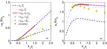
Figure 4: Comparisons of point dipole simulation result with dispersion relation solutions with different types of bounce averages of $\omega_{D}$ and $J_{0}$.

Figure 4 shows further comparison of the simulation result with different type of bounce averages of the dispersion relation. We can find that the results are mainly affected by the bounce average of $\omega_{D}$, and the growth rate is larger after bounce average which agree with the simulation result in Fig.3(d). The bounce average of $J_{0}$ affects little to the real frequency and growth rate. Fig.5 shows the corresponding mode structures for different $k_{\perp}\rho_{i}$, which shows that the mode structures are not flat with $k_{\perp}\rho_{i}$ increasing and thus the $k_{\parallel}=0$ assumption will be broken. This may explain the larger deviation of the $\omega$ in Fig.4 for larger $k_{\perp}\rho_{i}$. Fig.6 shows the corresponding mode structures for different $x_{c}$, where the $k_{\parallel}=0$ assumption also not always holds.

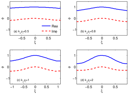
Figure 5: Mode structures for $\kappa_{n}=5.0$, $\kappa_{T}=0.0$ at point dipole with $k_{\perp}\rho_{i}=0.5$, $0.8$, $1.0$ and $2.0$ respectively.

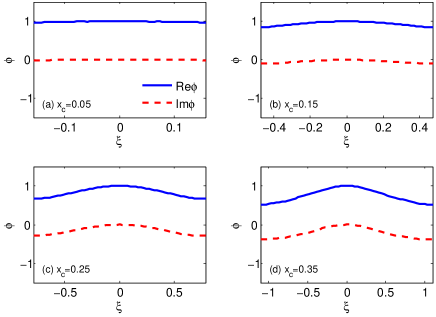
Figure 6: Mode structures for $\kappa_{n}=5.0$, $\kappa_{T}=0.0$ at point dipole with $x_{c}=0.05$, $0.15$, $0.25$ and $0.35$ respectively.

The mode in scanning $x_{c}$ in Fig.3 only has slight quantitative change of real frequency and growth rate. This tells us that the physical feature of this mode does not depend on whether the particles are trapped or passing. Thus, if we ignore the influence of the mode structures, we can expect that the general picture of the electrostatic drift modes in dipole configuration (all are trapped particles) be similar to the one in Z-pinch (all are passing particles) as studied in Ref.Ricci2006 and more details in Ref.Xie2017a , i.e., only two types of unstable electrostatic drift modes in the system, one is mainly driven by electron gradient and propagates in electron diamagnetic direction; and another is mainly driven by ion gradient and propagates in ion direction. However, when considering the mode structures, we find some new physics not existed in Z-pinch configuration, i.e., high order eigenstates of the mode can be more unstable than the ground state in particular parameters.

The modes property in $(\kappa_{n},\kappa_{T})$ space with $k_{\perp}\rho_{i}=0.5$ is shown in Fig.7, which is obtained from dispersion relation with matrix method as described in Ref.Xie2017a with only bounce averaged for $\omega_{D}$ not for $J_{0}$. In this figure we can find two unstable modes exist, one is in electron direction and another is in ion direction and the unstable threshold for both $\kappa_{n}$ and $\kappa_{T}$ are around $5.0$. The $\omega_{r}<0$ ion direction mode in Fig.7(a&b) can be unstable for either larger $\kappa_{n}$ or $\kappa_{T}$; whereas the $\omega_{r}>0$ electron direction mode in Fig.7(c&d) is only unstable when $\eta=\kappa_{T}/\kappa_{n}$ is large.

We notice that this is opposite as the case in tokamak community. In tokamakGarbet2006 , the ion (diamagnetic) direction ion temperature gradient mode (ITG) is only unstable at large $\eta$, whereas the electron direction trapped electron mode (TEM) can be unstable with the $\eta=0$ density gradient driven alone.

VII Parameters scan in Simulations

In this section, we study details of the linear electrostatic drift modes in the dipole configuration. In our simulations, we find the qualitative features of these electrostatic drift modes are similar between point dipole and ring dipole. And the differences are only quantitatively. Thus, we mainly focus on point dipole case. Firstly we scan $\eta$ to confirm that two types of mode exist in the system. Figure 8 shows the results with $\kappa_{n}=5.0$, $k_{\perp}\rho_{i}=1.0$, $x_{c}=0.35$, $n_{p}=5\times 10^{5}$ $n_{g}=64$, $dt=0.0002$ and $n_{t}=3\times 10^{5}$. We can see that indeed there exists a transition from ion mode with negative frequency to electron mode with positive frequency at around $\eta\sim\eta_{c}=2/3$. In Fig.7, we know that both electron and ion modes can be unstable at large $\eta$. The results of scan $k_{\perp}\rho_{i}$ for a typical large $\eta$ are shown in Fig.9, where we find that the ion mode is dominant at small $k_{\perp}\rho_{i}$ and the electron mode becomes dominant at larger $k_{\perp}\rho_{i}$. The dispersion relation can still predict the qualitative features of these two modes. In Fig.9, we have also shown the adiabatic electron model ($ns=1$) results, which is in the ion direction. Although the real frequency can roughly agree with the kinetic electron model ($ns=2$) results, the behavior of the growth rate is much different between these two models. This tells us that the electrostatic drift modes in dipole configuration can not be described by adiabatic electron model. Figure 10 shows the corresponding mode structures by scanning $\eta$ and the structure of $ns=1$ mode is much center peaked and not flat as the $ns=2$ mode. Here and after, the dispersion relation results in point dipole are all obtained with bounce averaged only for $\omega_{D}$ and not for $J_{0}$. In the latter part, we will mainly focus on the $\eta<\eta_{c}$ mode.

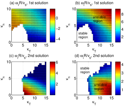
Figure 7: Scan $(\kappa_{n},\kappa_{T})$ in point dipole using dispersion relation, with $k_{\perp}\rho_{i}=0.5$. Two branches of unstable mode exist: one in ion direction (a&b) and another in electron direction (c&d).

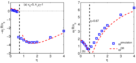
Figure 8: Scan $\eta=\kappa_{T}/\kappa_{n}$ in point dipole and comparison with dispersion relation solution.

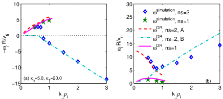
Figure 9: Scan $k_{\perp}\rho_{i}$ in point dipole at $\eta=4$. With the comparison of kinetic electron model ($ns=2$) and adiabatic electron ($ns=1$) model.

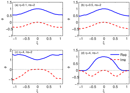
Figure 10: Mode structures for $\kappa_{n}=5.0$, $k_{\perp}=1.0$ at point dipole with $\eta=0.1$, $0.5$, $4.0$ with $ns=2$ and $\eta=4.0$ with $ns=1$ respectively.

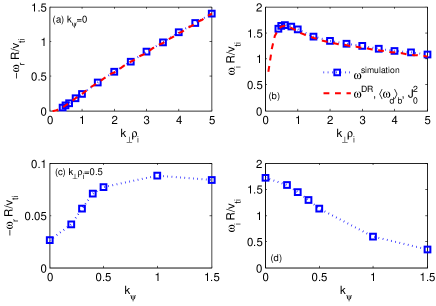
Figure 11: Scan of $k_{\perp}\rho_{i}$ and $k_{\psi}$, with $\kappa_{n}=5.0$ and $\kappa_{T}=1.0$ in point dipole.

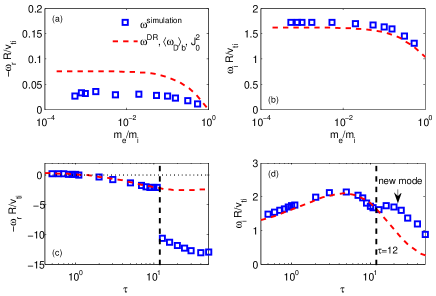
Figure 12: Scan of $m_{e}/m_{i}$ and $\tau$, with $\kappa_{n}=5.0$, $\kappa_{T}=1.0$ and $k_{\perp}\rho_{i}=0.5$ in point dipole.

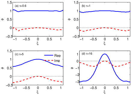
Figure 13: Mode structures for $\kappa_{n}=5.0$, $\kappa_{T}=1.0$ and $k_{\perp}\rho_{i}=0.5$ in point dipole with $\tau=0.5$, $1$, $5$ and $16$ respectively.

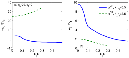
Figure 14: Scan of $k_{\parallel}R$ using the dispersion relation Eq.(22), with $\kappa_{n}=20$ and $\kappa_{T}=0$ in point dipole, for $k_{\perp}\rho_{i}=0.5$ and $k_{\perp}\rho_{i}=2.5$.

Figure 11 shows the scan of $k_{\zeta}$ and $k_{\psi}$. The result for $k_{\zeta}$ scanning agrees with the typical entropy mode feature in Ref.Ricci2006 ; Xie2017a , and especially for large $k_{\perp}\rho_{i}$ the mode is still unstable. The most unstable solution exists at $k_{\perp}\rho_{i}\simeq 1.0$. The $k_{\psi}$ scan does not bring any qualitative difference but play a role in increasing $k_{\perp}$ [see Eq.(B)]. Figure 12(a&b) shows the scan of $m_{e}/m_{i}$. We find that at small $m_{e}/m_{i}<0.01$ the simulation results of $\omega_{r}$ and $\gamma$ change little. Whereas the scan of $\tau$ in Fig.12(c&d) show something interesting, i.e., a new mode become unstable at $\tau>12$. And around $\tau=12$, two modes compete in the simulation. The real frequency is very small at $\tau\sim 1$, where a smooth sign change from ion direction to electron direction is observed. By scan $\tau$ in dispersion relation solver, we only find one unstable mode, i.e., this new mode may not exist in the zero-dimensional model and must have something to do with the mode structure. We find indeed that these two modes have different mode structures. As shown in Fig.13, at small $\tau$ ($\tau=0.6$ and $1.0$) the mode structure of $\phi(\xi)$ is flat; at mediate $\tau$ ($\tau=5.0$) $\phi(\xi)$ is much similar as the one in Fig.5(d) and Fig.6(d); for large $\tau$ ($\tau=16>\tau_{c}\simeq 12$) the mode structure changes more, e.g., both $Re\phi(\xi)>0$ and $Re\phi(\xi)<0$ exist. This jump also exists in ring dipole case. This new mode may be the high order eigenstate of the original ground state mode. We will show that series of high order eigenstates indeed exist in the system and can be the most unstable one. As shown in Fig.14, we scan the zero-dimensional dispersion relation Eq.(22) with $k_{\parallel}\neq 0$ and find that only one unstable mode exists and the $k_{\parallel}$ only brings damping effect because of electron Landau damping. This implies that this one-dimensional new mode in Fig.12(c&d) can not be predicted by zero-dimensional dispersion relation.

By increasing density gradient $\kappa_{n}$ in Fig.15, we find the most unstable mode in the system can have very different mode structures. Fig.15(a) shows the ground mode; Fig.15(b&c) show high-order even mode; and Fig.15(d) shows high-order odd mode. Considering that the result may be affected by $x_{c}$ in the point dipole simulation, we study this feature in detail using ring dipole configuration with $x_{c}=1.0$, i.e., to remove the effects of the boundary condition. Figure 16 shows a scan of $k_{\perp}\rho_{i}$ in the ring dipole configuration with $\kappa_{n}=50$. We see that the dispersion relation only predicts an unstable mode at $k_{\perp}\rho_{i}<1.5$, which qualitatively agrees with the $l=0$ mode in simulation. The slab dispersion relation is used to obtain $\omega^{\rm theory}$, but we have used the curvature drift frequency at $\xi=0$, i.e., $\omega_{d}^{\rm ring}=g(0)\omega_{d}^{\rm Z-pinch}$ with $g(0)=1.31$. However, new unstable modes appear by increasing $k_{\perp}\rho_{i}$ in the simulation, and the corresponding mode structures are shown in Fig.17. Due to steep gradient, this mode is ‘interchange-like’ Xie2017a , as $\omega_{i}\to\gamma_{0}\neq 0$ for $k_{\perp}\rho_{i}\to 0$. The eigenstate label $l$ here is roughly to fit the mode structure with $\phi(\xi)=H_{l}(\xi)e^{-\xi^{2}/2}$, where $H_{l}$ is $l$-th Hermite polynomials, with $l=0,1,2,\cdots$. That is, under strong gradient or large $\tau$, the most unstable mode in the system can be on non-ground state and the assumption $k_{\parallel}=0$ is not valid any more, which is not predicted by conventional understandings (cf. Refs.Kobayashi2009 ; Kesner2002 ). These high order eigenstates have been predicted in tokamak edge steep gradient parameters recentlyXie2015 where the physical explanation of it is the change of quantum potential well, and which can also change the nonlinear transport feature Xie2017 . It is also interesting that the even mode and odd mode have opposite propagation directions in Fig.17. The physical reason for why these high order modes can be most unstable is yet to study. The drift-bounce resonance $\omega-p\omega_{b}-q\omega_{D}=0$ with $p,q=0,\pm 1,\pm 2,\cdots$ in Refs.Dettrick2003 ; Zhu2014 is one possibility. However, we did not find clear resonant structures in $g_{i,e}(E,\lambda)$ velocity space as in Ref.Zhu2014 yet. The velocity space resonance in both Refs.Dettrick2003 ; Zhu2014 is between energetic ions and electromagnetic Alfvén mode, whereas our simulation includes only background ions and electrostatic perturbations. It is also not clear yet how this high order modes affect the nonlinear physics in dipole plasma.

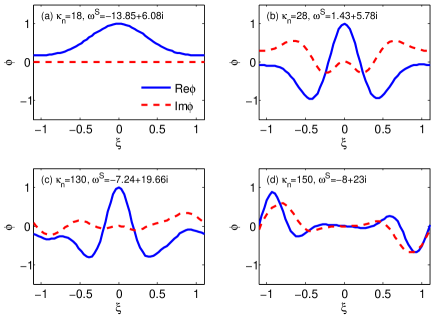
Figure 15: High order eigenstates mode exist at strong gradient with $\kappa_{T}=0.0$, $k_{\perp}=2.5$ and $\kappa_{n}=18$, $28$, $130$ and $150$ respectively in point dipole configuration.

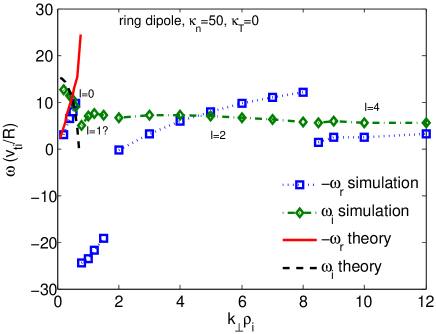
Figure 16: Scanning $\omega$ vs. $k_{\perp}\rho_{i}$ for $\kappa_{n}=50$, $\kappa_{T}=0$ in ring dipole configuration. High order modes are most unstable for large $k_{\perp}\rho_{i}$.

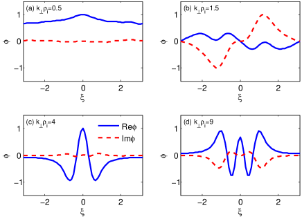
Figure 17: Corresponding mode structures vs. $k_{\perp}\rho_{i}$ for $\kappa_{n}=50$, $\kappa_{T}=0$ in ring dipole configuration.

VIII Summary and Conclusion

In this work, we have developed a 1D linear local collisionless gyrokinetic $\delta f$ PIC code to study the electrostatic drift modes in a point and ring dipole plasmas. With assumption of $k_{\parallel}=0$, the corresponding 0D bounce averaged dispersion relation is also derived and solved for benchmark. We find the general feature of the electrostatic drift modes in dipole configuration is similar to the one in Z-pinch configuration, i.e., two unstable modes exist mainly at either small $\eta$ or large $\eta$ with critical $\eta_{c}\simeq 2/3$. However, there still exists much difference between dipole and Z-pinch configurations. In Z-pinch, $k_{\parallel}\simeq 0$ is a good approximation; whereas for point and ring dipole, $k_{\parallel}\simeq 0$ is only valid at very narrow parameter space, e.g., only for small $k_{\perp}\rho_{i}$. Some new unstable modes with non-flat mode structure are found in dipole configuration at large $\tau$ and $\kappa_{n}$. With a smooth change of the temperature ratio $\tau=T_{e}/T_{i}$ from 0.5 to 60, we find a jump in real frequency and a turning point in growth rate at around $\tau=\tau_{c}\simeq 12$ which is caused by the competition between two different modes. More clearly, we have demonstrated that the most unstable mode is at high order eigenstates with either odd parity or even parity at large $\kappa_{n}$, as has been predicted Xie2015 in tokamak configuration.

We also notice that one major difference between dipole configuration and tokamak is the magnetic shear $s=0$. For $s\neq 0$ as in tokamak, the parallel boundary condition in the simulation model should be modifiedBeer1995 ; Chen2003 and the physics can be different. And the ITG and TEM in tokamak usually have $k_{\parallel}\neq 0$. What we think is interesting is that although almost all the particles are trapped in the dipole configuration, we have not found new mode can be called as trapped electron modeCoppi1974 as in tokamak. The essential unstable electrostatic drift modes in dipole configuration is similar to the one in Z-pinch configuration where all particles are passing particles.

In summary, we have given a comprehensive linear study of the 1D electrostatic drift modes in a point and ring dipole plasma. This helps us to understand the basic linear behaviors of the unstable modes in the system and can provide a starting point for further nonlinear study. Contrast to previous studies Kesner2000 ; Simakov2001 , this work is valid for all the gyrokinetic orderings, without further approximations. Contrast to previous Z-pinch and ring dipole studiesRicci2006 ; Kobayashi2009 ; Kobayashi2010 ; Xie2017a , this work demonstrates the importance of the parallel mode structures and finds that the high order eigenstates can be important at some parameters.

Appendix A Current loop/ring dipole magnetic field

We consider the dipole magnetic field produced by single current loop Jackson1999 with radius $a$. In cylinder coordinate $(\rho,\phi,z)$, for current density

$${\bf{J}}=I\delta\left({z^{\prime}}\right)\delta\left({\rho^{\prime}-a}\right)\left({-\sin\phi^{\prime},\cos\phi^{\prime},0}\right),$$ (23)

we have the magnetic vector potential

$${\bf{A}}={{{\mu_{0}}}\over{4\pi}}\int{{{{\bf{J}}\left({{\bf{r^{\prime}}}}\right)}\over{\left|{{\bf{r}}-{\bf{r^{\prime}}}}\right|}}{d^{3}}{\bf{r^{\prime}}}},$$ (24)

where $a$ is the radius of the current loop.

Due to symmetry, magnetic vector has only $\phi$ component, and

$${A_{\phi}}={{{\mu_{0}}I}\over{2\pi}}\sqrt{{a\over\rho}}\left[{{{\left({{k^{2}}-2}\right)K\left({{k^{2}}}\right)+2E\left({{k^{2}}}\right)}\over{2k}}}\right],$$ (25)

where $K$ and $E$ are the first and second kind of elliptic functions with

$$k^{2}=\frac{4a\rho}{(a+\rho)^{2}+z^{2}},~{}~{}\rho^{2}=x^{2}+y^{2}.$$ (26)

Hence, we obtain the magnetic field

$${{\bf{B}}_{{\rm{singlecoil}}}}=\nabla\times{\bf{A}}=-{{\partial{A_{\phi}}}\over{\partial z}}\hat{\rho}+{1\over\rho}{{\partial\left({\rho{A_{\phi}}}\right)}\over{\partial\rho}}\hat{z}.$$ (27)

Using

$$\left\{\begin{aligned} K^{\prime}\left(x\right)&={1\over{2x\left({1-x}\right)}}E\left(x\right)-{1\over{2x}}K\left(x\right),\\ E^{\prime}\left(x\right)&={1\over{2x}}E\left(x\right)-{1\over{2x}}K\left(x\right),\\ \end{aligned}\right.$$ (28)

we obtain

$$\left\{\begin{aligned} {B_{\rho}}&={{{\mu_{0}}I}\over{2\pi}}{z\over{\rho\sqrt{{{\left({a+\rho}\right)}^{2}}+{z^{2}}}}}\left[{{{{a^{2}}+{\rho^{2}}+{z^{2}}}\over{{{\left({a-\rho}\right)}^{2}}+{z^{2}}}}E\left({{k^{2}}}\right)-K\left({{k^{2}}}\right)}\right],\\ {B_{z}}&={{{\mu_{0}}I}\over{2\pi}}{1\over{\sqrt{{{\left({a+\rho}\right)}^{2}}+{z^{2}}}}}\left[{{{{a^{2}}-{\rho^{2}}-{z^{2}}}\over{{{\left({a-\rho}\right)}^{2}}+{z^{2}}}}E\left({{k^{2}}}\right)+K\left({{k^{2}}}\right)}\right],\\ {B_{\phi}}&=0.\end{aligned}\right.$$ (29)

And the magnetic flux can be calculated as $\psi=\oint{\bm{B}}\cdot d{\bm{S}}=\oint(\nabla\times{\bm{A}})\cdot d{\bm{S}}=\oint{\bm{A}}\cdot d{\bm{l}}=2\pi RA_{\phi}$, which would be used to determine the flux surface. For practise usage, we calculate the field line functions numerically and use interpolation basing on the above formula.

Appendix B Point dipole operators

Comparing to the ring dipole configuration equations in Sec.III, the benefit of using ideal point dipole configuration is that all the operators we used in the numerical code can be obtained analytically. We can have the following orthogonal flux coordinate $(\psi,\chi,\zeta)$ for ideal point dipole configuration

$$\left\{\begin{split}\psi&=\frac{M\sin^{2}\theta}{r},\\ \chi&=\frac{M\cos\theta}{r^{2}},\\ \zeta&=\phi,\end{split}\right.~{}~{}\left\{\begin{split}{\bm{e}}^{\psi}&=\nabla\psi=\frac{M\sin\theta}{r^{2}}(-\sin\theta{\bm{\hat{}}e}_{r}+2\cos\theta{\bm{\hat{}}e}_{\theta}),\\ {\bm{e}}^{\chi}&=\nabla\chi=-\frac{M}{r^{3}}(2\cos\theta{\bm{\hat{}}e}_{r}+\sin\theta{\bm{\hat{}}e}_{\theta}),\\ {\bm{e}}^{\zeta}&=\nabla\zeta=\frac{1}{r\sin\theta}{\bm{\hat{}}e}_{\phi},\end{split}\right.$$ (30)

where $M$ is the magnetic moment of the dipole, and $(r,\theta,\phi)=(radial,polar,azimuthal)$ is spherical coordinates with ${\bm{\hat{}}e}_{r}$, ${\bm{\hat{}}e}_{\theta}$ and ${\bm{\hat{}}e}_{\phi}$ the unit vector in each directions. Note that ${\bm{B}}=\nabla\phi\times\nabla\psi=\nabla\chi$ and $B=\sqrt{{\bm{B}}\cdot{\bm{B}}}=(M/r^{3})\sqrt{1+3\cos^{2}\theta}$.

For completeness, besides the contravariant vector ${\bm{e}}^{\alpha}=\nabla\alpha$, we also list here the covariant vector ${\bm{e}}_{\alpha}=\partial_{\alpha}{\bm{r}}$

$$\left\{\begin{split}{\bm{e}}_{\psi}&=\partial_{\psi}{\bm{r}}=\frac{r^{2}(-\sin\theta{\bm{\hat{}}e}_{r}+2\cos\theta{\bm{\hat{}}e}_{\theta})}{M\sin\theta(1+3\cos^{2}\theta)},\\ {\bm{e}}_{\chi}&=\partial_{\chi}{\bm{r}}=-\frac{r^{3}(2\cos\theta{\bm{\hat{}}e}_{r}+\sin\theta{\bm{\hat{}}e}_{\theta})}{M(1+3\cos^{2}\theta)},\\ {\bm{e}}_{\zeta}&=\partial_{\zeta}{\bm{r}}=r\sin\theta{\bm{\hat{}}e}_{\phi},\end{split}\right.$$ (31)

with also ${\bm{e}}^{\alpha}\times{\bm{e}}^{\beta}=\mathcal{J}^{-1}{\bm{e}}_{\gamma}$ and ${\bm{e}}^{\alpha}\cdot{\bm{e}}_{\beta}=\delta^{\alpha}_{\beta}$. And it is readily to obtain the contravariant metric tensor $g^{\alpha\beta}\equiv\nabla\alpha\cdot\nabla\beta$, the covariant metric tensor $g_{\alpha\beta}\equiv\partial_{\alpha}{\bm{r}}\cdot\partial_{\beta}{\bm{r}}$, and the Jacobian $\mathcal{J}\equiv{\bm{e}}_{\alpha}\cdot{\bm{e}}_{\beta}\times{\bm{e}}_{\gamma}=1/\sqrt{\det(g^{\alpha\beta})}=\sqrt{\det(g_{\alpha\beta})}=\frac{r^{6}}{M^{2}(1+3\cos^{2}\theta)}$. Note also $g_{\alpha\beta}g^{\beta\gamma}=\delta_{\alpha}^{\gamma}$, ${\bm{e}}_{\alpha}=g_{\alpha\beta}{\bm{e}}^{\beta}$, ${\bm{e}}^{\alpha}=g^{\alpha\beta}{\bm{e}}_{\beta}$, ${\bm{e}}_{\alpha}\times{\bm{e}}_{\beta}=\mathcal{J}\varepsilon_{\alpha\beta\gamma}{\bm{e}}^{\gamma}$ and ${\bm{e}}^{\alpha}\times{\bm{e}}^{\beta}=\mathcal{J}^{-1}\epsilon^{\alpha\beta\gamma}{\bm{e}}_{\gamma}$. Considering covariant ${\bm{B}}=B_{\alpha}{\bm{e}}^{\alpha}$ ($B_{\alpha}={\bm{B}}\cdot{\bm{e}}^{\alpha}$) and contravariant ${\bm{B}}=B^{\alpha}{\bm{e}}_{\alpha}$ ($B^{\alpha}={\bm{B}}\cdot{\bm{e}}_{\alpha}$), we can have ideal dipole field ${\bm{B}}={\bm{e}}^{\chi}=\mathcal{J}^{-1}{\bm{e}}_{\chi}$, which is true because ${\bm{B}}=\nabla\psi\times\nabla\zeta$ and $\nabla\psi\times\nabla\zeta=\mathcal{J}^{-1}\partial_{\chi}{\bm{r}}$, and we obtain

$$\left\{\begin{split}B^{\chi}&=\mathcal{J}^{-1}=\frac{M^{2}(1+3\cos^{2}\theta)}{r^{6}},\\ B^{\psi}&=0,\\ B^{\zeta}&=0,\end{split}\right.~{}~{}~{}~{}~{}~{}\left\{\begin{split}B_{\chi}&=1,\\ B_{\psi}&=0,\\ B_{\zeta}&=0,\end{split}\right.$$ (32)

with magnetic vector ${\bm{A}}=-\psi\nabla\zeta$, i.e., $\nabla\times{\bm{A}}=-\nabla\times\psi\nabla\zeta=\nabla\zeta\times\nabla\psi={\bm{B}}$.

Along a field line $l$, $\psi$ and $\zeta$ do not change, and we can still obtain $dl=r_{0}\kappa(\xi)d\xi$, where $\xi=\pi/2-\theta$, $\kappa=\cos\xi(1+3\sin^{2}\xi)^{1/2}$ and $r_{0}$ is the distance from the flux surface to the origin at the equator $\xi=0$. Note that here $\xi\in(-\pi/2,\pi/2)$, which differs from the ring dipole case $\xi\in[-\pi,\pi]$. We can readily obtain $f(\xi)=B/B_{0}=\frac{\sqrt{1+3\sin^{2}\xi}}{\cos^{6}\xi}$, and

$$k_{\perp}^{2} = k_{\psi}^{2}\nabla\psi\cdot\nabla\psi+k_{\zeta}^{2}\nabla\zeta\cdot\nabla\zeta$$

$$= \frac{1}{r_{0}^{2}\cos^{6}\xi}\Big{[}k_{\zeta}^{2}+k_{\psi}^{2}{B_{0}^{2}r_{0}^{4}}(1+3\sin^{2}\xi)\Big{]},$$

where we have used Eq.(30), $r=r_{0}\sin^{2}\theta$ and $B_{0}=M/r_{0}^{3}$. Here, we have $\rho_{s}=\frac{v\sqrt{\lambda}}{\Omega_{s0}}\Big{|}\frac{\cos^{3}\xi}{(1+3\sin^{2}\xi)^{1/4}}\Big{|}$ and consider $k_{\psi}\neq 0$, and thus

$$k_{\perp}\rho_{s}=\frac{v\sqrt{\lambda}}{r_{0}\Omega_{s0}}\sqrt{k_{\zeta}^{2}+k_{\psi}^{2}{B_{0}^{2}r_{0}^{4}}z}\frac{1}{z^{1/4}},$$

$$\partial_{\xi}(k_{\perp}\rho_{s})=\frac{v\sqrt{\lambda}}{r_{0}\Omega_{s0}}\frac{-k_{\zeta}^{2}+k_{\psi}^{2}{B_{0}^{2}r_{0}^{4}}z}{4z^{5/4}\sqrt{k_{\zeta}^{2}+k_{\psi}^{2}{B_{0}^{2}r_{0}^{4}}z}}6\sin\xi\cos\xi,$$

and

$$b_{s}=\Big{(}\frac{k_{\perp}v_{ts}}{\Omega_{s}}\Big{)}^{2}=\frac{v_{ts}^{2}}{r_{0}^{2}\Omega_{s0}^{2}}\Big{[}k_{\zeta}^{2}+k_{\psi}^{2}{B_{0}^{2}r_{0}^{4}}z\Big{]}\frac{\cos^{6}\xi}{z},$$

with $z=1+3\sin^{2}\xi$.

The $\omega_{*s}^{T}$ is the same as in the ring dipole case. The gradient drift ${\bm{v}}_{g}$, curvature drift ${\bm{v}}_{c}$ and total drift ${\bm{v}}_{d}={\bm{v}}_{g}+{\bm{v}}_{c}$ can be calculated as

$${\bm{v}}_{g}=\frac{1}{m\Omega_{s}}\mu{\bm{b}}\times\nabla B=-\frac{v_{\perp}^{2}}{2\Omega_{s}}(\partial_{\psi}B){\bm{e}}_{\zeta},$$

$${\bm{v}}_{c}=\frac{1}{\Omega_{s}}v_{\parallel}^{2}\nabla\times{\bm{b}}=-\frac{v_{\parallel}^{2}}{\Omega_{s}}(\partial_{\psi}B){\bm{e}}_{\zeta},$$

$${\bm{v}}_{d}=-\frac{3(\cos^{2}\theta+1)\sin^{5}\theta}{r_{0}\Omega_{s0}(1+3\cos^{2}\theta)^{2}}(v_{\parallel}^{2}+\frac{1}{2}v_{\perp}^{2}){{\hat{e}}_{\phi}},$$

where we have used $\partial_{\psi}B=\frac{3(\cos^{2}\theta+1)}{r^{2}(1+3\cos^{2}\theta)^{3/2}}$ and ${\bm{e}}_{\zeta}=\partial_{\zeta}{\bm{r}}=r\sin\theta{{\hat{e}}_{\phi}}$. And thus

$$\omega_{Ds}={\bf k_{\perp}}\cdot{\bm{v}}_{d}=-\omega_{d0}\frac{3(1-\sin^{4}\xi)}{(1+3\sin^{2}\xi)^{2}}\frac{(1+y)}{2}v^{2},$$ (34)

with $\omega_{d0}=\frac{k_{\zeta}}{r_{0}^{2}\Omega_{s0}}$.

We use the same normalization as in the ring dipole case and the expression for all other variables are the same, except $\epsilon_{n}\equiv-\frac{1}{B_{0}r_{0}^{2}}\Big{(}\frac{\partial\ln n_{0}}{\partial\psi}\Big{)}^{-1}=L_{n}/B_{0}r_{0}^{2}$ and $k_{\psi}\to k_{\psi}B_{0}r_{0}^{2}$. And hence

$$k_{\perp}^{2}=(k_{\zeta}^{2}+k_{\psi}^{2}z)/\cos^{6}\xi,$$

$$k_{\perp}\rho_{s}=\frac{v}{v_{ts}}\sqrt{\lambda}\sqrt{(k_{\zeta}^{2}+k_{\psi}^{2}z)}z^{-1/4}\rho_{ts},$$

$$\partial_{\xi}(k_{\perp}\rho_{s})=\frac{v}{v_{ts}}\sqrt{\lambda}\frac{(-k_{\zeta}^{2}+k_{\psi}^{2}z)}{2z^{5/4}\sqrt{k_{\zeta}^{2}+k_{\psi}^{2}z}}3\sin\xi\cos\xi\rho_{ts}.$$

$$b_{s}=\rho_{ts}^{2}\Big{[}k_{\zeta}^{2}+k_{\psi}^{2}z\Big{]}\frac{\cos^{6}\xi}{z}.$$

Normalized curvature drift frequency is

$$\omega_{Ds}=-\omega_{ds0}\frac{3(1-\sin^{4}\xi)}{(1+3\sin^{2}\xi)^{2}}\frac{(1+y)}{2}\frac{v^{2}}{v_{ts}^{2}},$$

where $\omega_{di0}=k_{\zeta}\omega_{0}\rho_{ti}\to k_{\zeta}\rho_{ti}$ and $\omega_{de0}=\tau\frac{q_{i}}{q_{e}}\omega_{di0}$.

Appendix C Bounce average

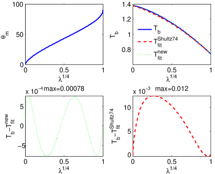
Figure 18: Turning point and bounce time.

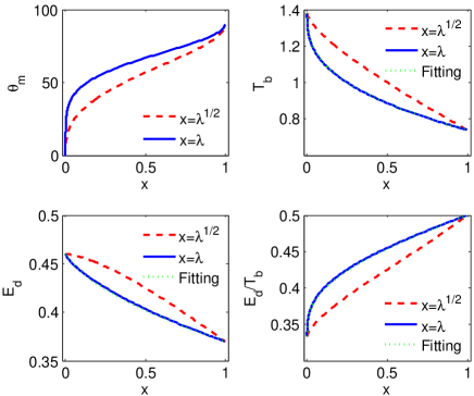
Figure 19: Drift integral.

Using $E$ and $\mu$ conserved, $v_{\parallel}=\sqrt{(2/m)(E-\mu B)}=v\sqrt{1-\lambda B/B_{0}}$, $v=\sqrt{2E/m}$, the bounce period is

$$T_{m}(r_{0},E,\lambda)=4\int_{\theta_{m}}^{\pi/2}\frac{dl}{d\theta}\frac{d\theta}{v_{\parallel}(\theta)}=\frac{4r_{0}}{v}T_{b}(\lambda),$$ (35)

which gives

$$T_{b}(\lambda)=\int_{\theta_{m}(\lambda)}^{\pi/2}\frac{\sin\theta(1+3\cos^{2}\theta)^{1/2}}{\Big{[}1-\lambda\frac{(1+3\cos^{2}\theta)^{1/2}}{\sin^{6}\theta}\Big{]}^{1/2}}d\theta,$$ (36)

where the turning point $\theta_{m}(\lambda)$ is determined by $v_{\parallel}=0$, i.e,

$$\frac{\sin^{6}\theta_{m}}{(1+3\cos^{2}\theta_{m})^{1/2}}=\lambda.$$ (37)

For $\lambda=0$, $T_{b}(0)=1+(\sqrt{3}/6)\ln(2+\sqrt{3})\simeq 1.38017$. For $\lambda=1$, the period can be calculated by small-amplitude oscillation $T_{b}(1)=(\pi/6)\sqrt{2}\simeq 0.74048$. Mirror force $F=\mu\nabla B$, gives $\frac{d^{2}s}{dt^{2}}=-\frac{\mu\nabla B}{m}=-\frac{\mu}{m}(\partial_{\chi}B)|{\bm{e}}^{\chi}|$. For deeply trapped particle, $\lambda\sim 1$, $\theta\sim\pi/2$, $ds\sim r_{0}d\theta$, and thus $\frac{d^{2}s}{dt^{2}}\simeq-\frac{v^{2}}{2}\frac{3\cos\theta(5\cos^{2}\theta+3)}{r(1+3\cos^{2}\theta)^{3/2}}\simeq-\frac{v^{2}}{2}\frac{9s}{r_{0}^{2}}$, which gives $T_{b}(\lambda=1)=(2\pi/\sqrt{\frac{9v^{2}}{2r_{0}^{2}}})/(4r_{0}/v)=\frac{\pi\sqrt{2}}{6}$. A fitting of $T_{b}(\lambda)$ can be found at Ref.Schulz1974

$$T_{b}(\lambda) \simeq T_{b}(0)-\frac{1}{2}[T_{b}(0)-T_{b}(1)](\lambda^{1/2}+\lambda^{1/4})$$ (38)

$$\simeq 1.3802-0.3198(\lambda^{1/2}+\lambda^{1/4}).$$

which gives a max error around $0.012$. We find a better fitting can be

$$T_{b}(\lambda)\simeq T_{b}(0)-\frac{1}{a+b+c}[T_{b}(0)-T_{b}(1)](a\lambda^{1/2}+b\lambda^{1/4}+c\lambda^{3/8}),$$ (39)

with $a=0.380$, $b=0.335$ and $c=1.0$, which gives a max error around $0.0008$, ten times better than the previous one, see Fig.18. The bounce frequency is given by

$$\omega_{b}=\frac{2\pi}{T_{m}}=\frac{\pi v}{2r_{0}}\frac{1}{T_{b}(\lambda)}.$$ (40)

In one bounce period, the angular displacement is

$$\Delta\phi=4\int_{\theta_{m}}^{\pi/2}\frac{dl}{d\theta}\frac{v_{d}(\theta)d\theta}{v_{\parallel}(\theta)r(\theta)\sin\theta},$$ (41)

and thus the angular drift velocity ($B_{0}=M/r_{0}^{3}$, $\Omega_{c}=eB/m$)

$$\omega_{d}=\frac{\Delta\phi}{T_{m}}=\frac{3mv^{2}}{eB_{0}r_{0}^{2}}\frac{E_{d}(\lambda)}{T_{b}(\lambda)},$$ (42)

where

$$E_{d}(\lambda)=\int_{\theta_{m}}^{\pi/2}\frac{\sin^{3}\theta(1+\cos^{2}\theta)\Big{[}1-\frac{1}{2}\lambda\frac{(1+3\cos^{2}\theta)^{1/2}}{\sin^{6}\theta}\Big{]}}{(1+3\cos^{2}\theta)^{3/2}\Big{[}1-\lambda\frac{(1+3\cos^{2}\theta)^{1/2}}{\sin^{6}\theta}\Big{]}^{1/2}}d\theta,$$ (43)

which agrees with Ref.Hamlin1961 . Result is shown in Fig.19. We can also calculate analytically $E_{d}(\lambda=0)=[6+\sqrt{3}\ln(2+\sqrt{3})]/18\simeq 0.460058$ and $E_{d}(\lambda=1)=\pi\sqrt{2}/12$. Compare Eqs.(36) and (43), $\frac{E_{d}(\lambda=1)}{T_{b}(\lambda=1)}=1-\frac{\lambda}{2}=\frac{1}{2}$.

We try the below fitting expression (see also Ref,Mauel2015 for similar fitting)

$$T_{b}(\lambda)\simeq T_{b}(0)+[T_{b}(1)-T_{b}(0)]\lambda^{3/8},$$ (44)

$$E_{d}(\lambda)\simeq E_{d}(0)+[E_{d}(1)-E_{d}(0)](\lambda^{3/8}+c\lambda^{1/2})/(1+c),~{}c=-2,$$ (45)

which seems can have max error less than $0.002$. Ref.Hamlin1961 also gives another two approximations: $T_{b}(\lambda)\simeq 1.30-0.56\lambda^{1/2}$ and $E_{d}(\lambda)/T_{b}(\lambda)\simeq 0.35+0.15\lambda^{1/2}$. In numerical aspects, we can also try high order polynomial fitting, e.g., using $\lambda^{1/8}$ as base.

The gyrokinetic dispersion relation in dipole field involve FLR effect and bounce average, i.e., Bessel function $\langle J_{0}(k_{\perp}\rho)\rangle_{b}$, where $\rho=\frac{mv_{\perp}}{qB}=\frac{m}{q}\sqrt{\frac{2\lambda E}{B_{0}B(\theta)}}=\frac{mv}{q}\sqrt{\frac{\lambda}{B_{0}B(\theta)}}$, i.e.,

$$J_{0b}(v,\lambda)=\frac{\int_{\theta_{m}}^{\pi/2}\frac{dl}{d\theta}\frac{J_{0}(k_{\perp}\rho)d\theta}{v_{\parallel}(\theta)}}{\int_{\theta_{m}}^{\pi/2}\frac{dl}{d\theta}\frac{d\theta}{v_{\parallel}(\theta)}}=\frac{\int_{\theta_{m}}^{\pi/2}\frac{dl}{d\theta}\frac{J_{0}\Big{(}k_{\perp}\frac{mv}{q}\sqrt{\frac{\lambda}{B_{0}B(\theta)}}\Big{)}d\theta}{v_{\parallel}(\theta)}}{\frac{r_{0}}{v}T_{b}(\lambda)}$$

$$=\frac{1}{T_{b}(\lambda)}\int_{\theta_{m}(\lambda)}^{\pi/2}\frac{J_{0}\Big{(}k_{\perp}\frac{mv}{q}\sqrt{\frac{\lambda}{B_{0}B(\theta)}}\Big{)}\sin\theta(1+3\cos^{2}\theta)^{1/2}}{\Big{[}1-\lambda\frac{(1+3\cos^{2}\theta)^{1/2}}{\sin^{6}\theta}\Big{]}^{1/2}}d\theta,$$ (46)

Note also that $J_{0b}\equiv\langle J_{0}(k_{\perp}\rho)\rangle_{b}\neq J_{0}(\langle k_{\perp}\rho\rangle_{b})$.

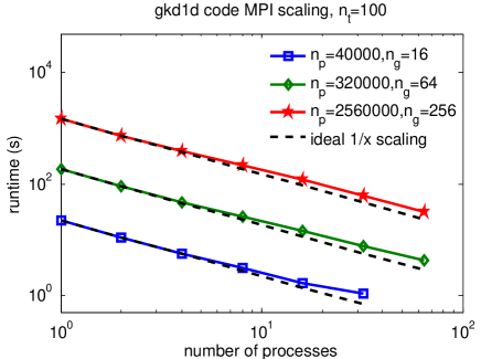
Figure 20: Gkd1d Fortran 90 code MPI scaling.

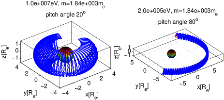
Figure 21: Typical charged particle trajectories under ideal dipole field in Earth shows good confinement even when the ion energy is large to 10MeV. Stochastic motion of particles due to the collision and turbulence can break this ideal confinement.

Appendix D MPI parallelization scaling

The gkd1d code is written using Fortran90 and with MPI (message passing interface) parallelization for particles. Thus this code could handle very large particle numbers. The parallelization performance is shown in Fig.20. In practise convergence test, we have used more than $n_{p}=10^{7}$ particles, and which is far adequate for most of our simulations. Usually, $n_{p}=10^{5}$ is enough for two species, $s=i,e$; and can even $n_{p}\leq 10^{4}$ for adiabatic electron case, i.e., $s=i$.

Appendix E Typical dipole orbits

Fig.21 shows two typical charged particle trajectories under ideal dipole field in Earth with the magnetic field $B(x=R_{e},y=0,z=0)=3.07\times 10^{5}T$, which shows good confinement even when the ion energy is large to 10MeV, where $R_{e}$ is the Earth radius.

Note: The blue text in only in this arXiv version, not included in the published Phys. Plasmas (2017) version.

References

(1) A. Hasegawa, Comments on Plasma
Physics and Controlled Fusion, 11, 147 (1987).
(2) A. Hasegawa, L. Chen and M. Mauel, Nucl. Fusion, 30,
2405 (1990).
(3) A. C. Boxer, D. T. Garnier, J. L. Ellsworth, J. Kesner, and M. E.
Mauel, J. Fusion Energy 27, 11 (2008).
(4) A. C. Boxer, R. Bergmann, J. L. Ellsworth, D. T. Garnier, J.
Kesner, M. E. Mauel and P. Woskov, Nat Phys, 6, 207 (2010).
(5) D. T. Garnier, M. E. Mauel, T. M. Roberts, J. Kesner and P. P. Woskov,
Phys. Plasmas, 24, 012506 (2017).
(6) B. Levitt, D. Maslovsky, and M. E. Mauel, Phys. Plasmas, 9, 2507
(2002).
(7) Z. Yoshida, Y. Ogawa, J. Morikawa, S. Watanabe, Y. Yano, S.
Mizumaki, T. Tosaka, Y. Ohtani, A. Hayakawa and M. Shibui, Plasma
and Fusion Research, 1, 008 (2006).
(8) Z. Yoshida, H. Saitoh, Y. Yano, H. Mikami, N. Kasaoka, W.
Sakamoto, J. Morikawa, M. Furukawa and S. M. Mahajan, Plasma Phys.
Control. Fusion, 55, 014018 (2013).
(9) G. Sarri, K. Poder, J.M. Cole, W. Schumaker,w, A. Di Piazza, B.
Reville, T. Dzelzainis, D. Doria, L.A. Gizzi, G. Grittani, S. Kar,
C.H. Keitel, K. Krushelnick, S. Kuschel, S.P.D. Mangles, Z.
Najmudin, N. Shukla, L.O. Silva, D. Symes, A.G.R. Thomas, M. Vargas,
J. Vieira and M. Zepf, Nature Communications, 6, 6747
(2015).
(10) J. Kesner, Phys. Plasmas, 5, 3675 (1998).
(11) J. Kesner, Phys. Plasmas, 7 3837 (2000).
(12) J. Kesner and R. J. Hastie, Phys. Plasmas, 9,
395 (2002).
(13) A. N. Simakov, P. J. Catto and R. J. Hastie, Phys. Plasmas, 8, 4414 (2001).
(14) P. Helander and J. W. Connor, Journal of Plasma Physics,
82, 905820301 (2016).
(15) W. Horton, Rev. Mod. Phys., 71, 735 (1999).
(16) S. Kobayashi, B. N. Rogers and W. Dorland, Phys. Rev.
Lett., 103, 055003 (2009).
(17) S. Kobayashi, B. N. Rogers and W. Dorland, Phys. Rev.
Lett., 105, 235004 (2010).
(18) A. N. Simakov, R. J. Hastie and P. J. Catto, Phys. Plasmas, 9,
201 (2002).
(19) S. Dettrick, L. J. Zheng and L. Chen, J. Geophys. Res., 108,
1150 (2003).
(20) P. Porazik and Z. Lin, Phys. Plasmas,
18, 072107 (2011).
(21) P. N. Mager and D. Y. Klimushkin, Plasma Phys. Control.
Fusion, 59, 095005 (2017).
(22) G. Zhao and L. Chen, “Gyrokinetic Particle-in-Cell Simulation of
Electrostatic Drift Modes in a Dipole Plasma”, 2001 International
Sherwood Fusion Theory Meeting, Santa Fe, New Mexico, 2001; G. Zhao,
Some Calculations for Dipole Simulation, unpublished notes, 2001.
(23) T. M. Antonsen and B. Lane, Phys. Fluids 23, 1205 (1980).
(24) L. Chen and A. Hasegawa, Journal Of Geophysical
Research, 96, 1503 (1991).
(25) H. S. Xie, Y. Y. Li, Z. X. Lu, W. K. Ou and B. Li, Phys. Plasmas,
24, 072106 (2017).
(26) S. E. Parker and W. W. Lee, Physics of Fluids B: Plasma Physics,
5, 77 (1993).
(27) P. H. Rutherford and E. A. Frieman, Physics of Fluids, 11,
569 (1968).
(28) P. Ricci, B. N. Rogers, W. Dorland, and M. Barnes, Phys. Plasmas, 13, 062102
(2006).
(29) A. Bierwage and L. Chen, Commun. Comput. Phys., 4,
457 (2008).
(30) H. S. Xie and Y. Xiao, Phys. Plasmas, 22, 090703 (2015).
H. S. Xie and B. Li, Phys. Plasmas, 23, 082513 (2016).
(31) H. S. Xie, Y. Xiao and Z. Lin, Phys. Rev. Lett., 118,
095001 (2017).
(32) J. Zhu, Z. W. Ma and G. Y. Fu, Nuclear Fusion, 54,
123020 (2014).
(33) M. A. Beer, S. C. Cowley, and G. W. Hammett, Phys. Plasmas 2, 2687
(1995).
(34) Y. Chen and S. E. Parker, Journal of Computational Physics, 189,
463 (2003).
(35) B. Coppi and G. Rewoldt, Phys. Rev. Lett. 33, 1329 (1974). P.
J. Catto and K. T. Tsang, Phys. Fluids 21, 1381 (1978).
(36) J. D. Jackson, Classical Electrodynamics, John Wiley & Sons.
Inc., New York, (1999).
(37) M. Schulz and L. J. Lanzerotti, Particle Diffusion in the Radiation
Belts, Springer-Verlag Berlin Heidelberg, 1974.
(38) D. A. Hamlin, R. Karplus, R. C. Vik and K. M. Watson,
Journal of Geophysical Research, 66, 1 (1961).
(39) M. E. Mauel, Drift orbits in a Symmetric Magnetic
Dipole, unpublished, 2015.