A Generalized Model for Light Transport in Scintillators
Abstract
Transported light in the medium usually shows as an exponential decay tendency. In the DAMPE strip scintillators, however, the phenomenon of light attenuation as the hit position approaches the end of the scintillator can not be described by the simple exponential decay model. The spread angle of PMT relative to hit position is distance-dependent, so the larger the angle, the larger the proportion of emitted light to becomes the effective input light. We consider the contribution of the spread angle, and propose a generalized model: . The model well describes the light attenuation in the scintillator, reducing the maximum deviation of the sample from the fit function from 29% to below 2%. Moreover, our model contains most of the traditional models, so the experimental data that traditional models can fit and our models fit well.
keywords:
Spread angle; Scintillator; PMT; Exponential decay; Hit position1 Introduction
Scintillation detector, as an important detector, is widely used in time-of-flight detector, position detector and electromagnetic calorimeter, including CMS at CERN[1], BESIII at HIEP[2], PSD and BGO at DAMPE[3, 4, 5, 6] et al. When particles enter the scintillator, the incident particle deposits part energy or all the energy, which causes ionization and excitation in a scintillator and emits fluorescence of a certain wave length. Then the emitted fluorescence propagates to the end of the scintillator and is collected by photomultiplier tube(PMT). Due to the particular importance of light transmission, various models have been tried to account for the decay of scintillators in the past few decades. It is worth mentioning that the double exponent(DE) model[8] and the reflected back(RB) model[9] are now generally accepted. Unfortunately, none of them well explain the anomalous enhancement of the light signals along the scintillator ends in DAMPE.
If the light transport can be clearly analyzed in a scintillator, we can accurately determine two important parameters – hit position and deposited energy. In this paper, because the spread angle of PMT relative to hit position is distance-dependent, we propose a generalized model of light transport in the scintillator. The model well describes the light attenuation in the scintillator, and is used to fit samples from PSD at DAPME [4, 5, 6], and gives the explanation of the phenomenon of samples different from the fitting function along the scintillator ends, which has not been explained well for many years.
The organization of this paper is as follows. A brief introduction about the exponential decay(ED) model, the double exponent(DE) model and the reflected back(RB) model in Sec.2. Sec.3 considers the contribution of the spread angle and gives our model about light transport in a scintillator. Sec.4 gives the result of our model. Sec.5 explains why is our new model so powerful. Finally, conclusion are given in Sec.6.
2 Traditional Models for Light Transport in Scintillators
The striped and the parallelepiped scintillators are the most widely used scintillators, including the calorimeter detector, time-of-flight detector and particle position detector. When particles hit the scintillator, the particle energy deposits in the scintillator. Then the atomic in the scintillator transition to the excited state, and back after excitation fluorescence, the emitted light is collected by the PMT at the end of the scintillator. Thus, the information of particles can be extracted by analyzing electronic information. It is generally known that transmitted light of an initial intensity in a medium can be described by an exponential decay(ED) function with a attenuation length:
In the traditional model, the striped scintillator is assumed to be a line of length . When the particle hits on the scintillator away from the PMT to the position, the collected light can be express as
| (1) |
And the deviation between fitting function and the sample can be described as
| (2) |
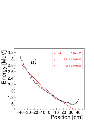
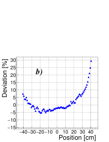
This ED model was used to fit samples of PSD on DAMPE [4, 5, 6], and showed a sharp increase in deviation as the hit position approaches the extremity of the scintillator. Therefore we searched for further physical models to fit the samples. In the past several decades, there are two further physical models: the Double Exponential(DE) model[8] and the Reflected Back(RB) model[9].
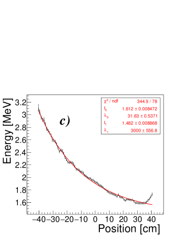
Kaiser et al proposed the DE model of light transmission with a short and a long attenuation length components described by the expression[8]
| (3) |
with being of the order of a few centimetres and ranging from 1 to several metres. Taiuti et al proposed the RB model that a fraction of the emitted light could be reflected back to the photomultiplier adding to the direct light a second component described by the expression[9]
| (4) |
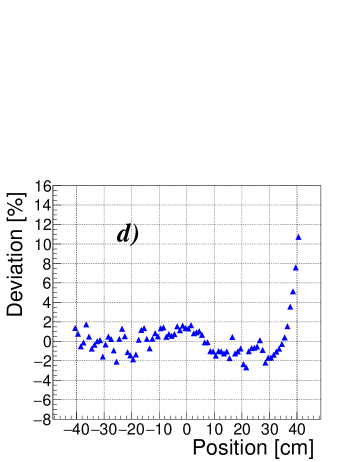
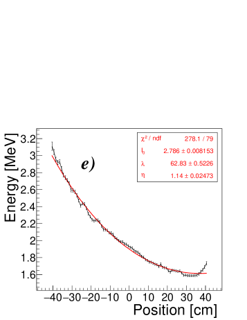
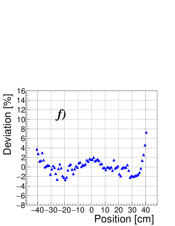
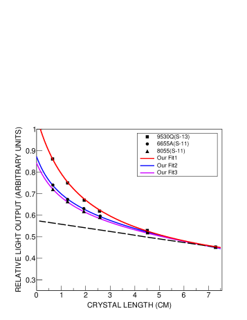
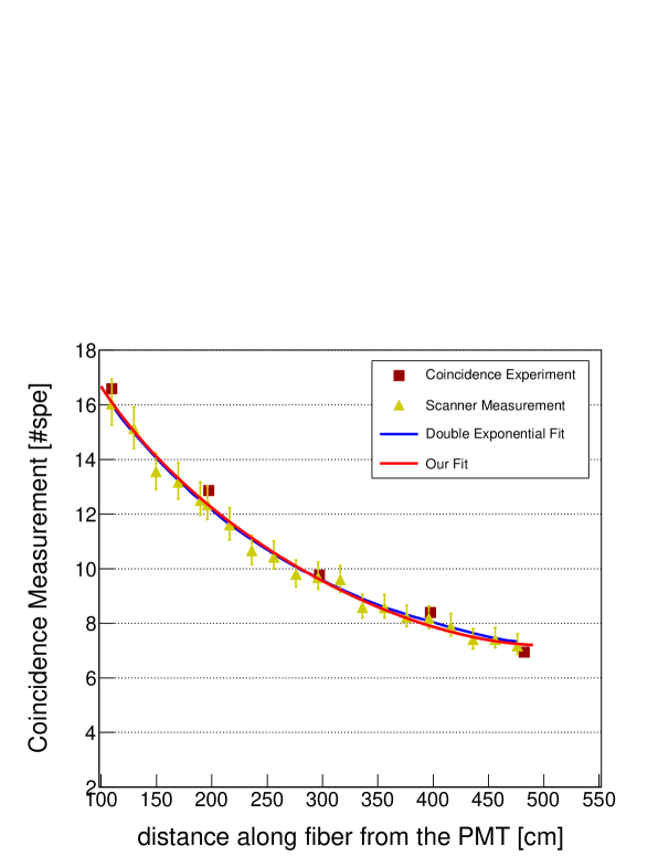
Both the DE model and the RB model had upgraded the ED model, and their deviations had been much reduced relative to the ED model. However, Fig.1 shows that there is a deviation of about for both models. In order to fit the samples, we consider the contribution of the spread angle and propose a generalized model in next section.
3 A Generalized Model for Light Transport in Scintillators
The optical signal intensity collected by PMT is related to the effective input light and the propagation loss. In this section, we point out that the effective light is -dependent. Where is the distance between hit position and the PMT.
When particles hit a scintillator, the spread angle of PMT relative to hit position is -dependent. Since the emitted light is uniformly distributed, the larger the spread angle, the larger the proportion of the emitted light becomes effective input light. Therefore, the contribution of the spread angle should be considered when describing the propagation of light in scintillators.
In traditional ED model, since the spread angle decreases as increases, we can simply multiply a fraction in place of the contribution of the spread angle. Where is less than .
If the emitted light may reflect back to the PMT as the RB model, the contribution of the spread angle should also be considered. Here the spread angle decreases as increases, so we can also simply multiply a fraction to replace the contribution of the spread angle. Where belongs to , is greater than and is the length of the scintillator.
So we can describe light propagation in scintillators as
| (5) |
where and represent the contribution from the spread angle.
4 Results
4.1 Fitting The Same Samples
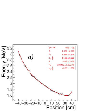
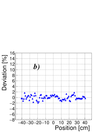
Fitting the same samples with our model, the deviation is reduced to less than 2%. Fig.2 and Table.1 show that this is far better than 29% of the ED model, 11% of the DE model and 7% of the RB model.
Table.1: Compare The Deviation With Other Models ED model DE model RB model our model 29% 11% 7% 2% 3644/80 344.9/78 278.1/79 93.4/76
4.2 More Experimental Data Fitting
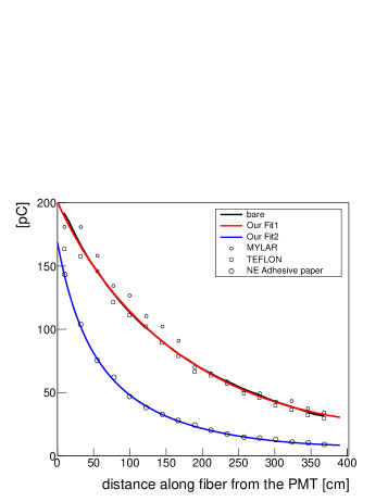
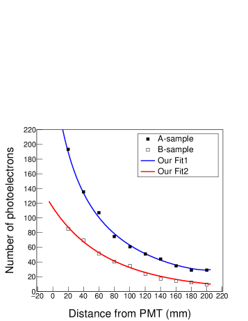
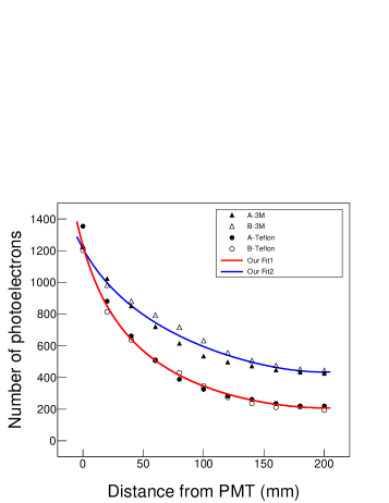
To show how powerful our model is, we describe more experimental data from different sources, including pilot B light output vs length using different PMT.[8], The effect of wrapping material on the light transmission for different materials [9], Light Transport in Long Plastic Scintillators[10], and plastic scintillator muon counters used in cosmic showers detection[11]. Fig.3-5 show that our model fits well with all the above experimental data.
5 Discussion
Why is our new model so generalized? Because the spread angle is an important physical factor that describes the light propagation in the scintillator, and this factor is considered in our new model. Moreover, our new model includes the three traditional models from Sec.2(see Appendix for details).
Case1:when and , our model can be degenerated to the ED model.
Case2:when and , our model can be degenerated to the RB model.
Case3:when , is about metres and larger than , our model can be approximately regarded to the DE model.
There is worth to mention that a semi empirical way the reflections of light at the ends of the scintillator was developed by R.Chipaux and M.Géléoc[12]. Our model can also be approximately regarded to this semi empirical way when . Therefore, our model can fit all experimental data that traditional models above can fit.
6 Conclusions
Our model for light transport in scintillators considers the contribution of the spread angle.
It can present the data from DAMPE to a great extent, and reduces the deviation between fitting function and the sample from 29% to less than 2%.
In addition, it contains the above traditional models. So it is stronger than the above traditional models,
and it can fit all data that the above traditional model can fit.
Acknowledgments:
This work are supported by the National Basic Research Program of China (973 Program) 2014CB845406, West Light Foundation of Chinese Academy of Sciences (Y532050XB0) and Key Research Program of Frontier Sciences, CAS, Grant NO.QYZDY-SSW-SLH006. One of us (J. Lan) thanks Z. Li, B. L. Zhang,
Z. W. Peng and Emilio CIUFFOLI for their help.
Appendix: For case1, , then , our model can be degenerated to the ED model.
For case2, , then , our model can be degenerated to the RB model.
For case3, , use to replace , with being about metres and larger than . For the DE model, with being of the order of a few centimetres and ranging from 1 to several metres, .
for ;
, for .
Adjusting the parameters and such that for , and for , our model can be approximately regarded to the DE model.
References
- [1] Della Negra, Michel; Petrilli, Achille; Herve, Alain; Foa, Lorenzo. CMS Physics Technical Design Report Volume I: Software and Detector Performance.(2006).
- [2] M. Ablikim et al., Design and construction of the BESIII detector, Nucl. Instrum. Meth. A 614(2010) 345.
- [3] J. Chang, Dark matter particle explorer the first Chinese cosmic ray and hard -ray detector in space, Chin. J. Space Sci. 34 (5) (2014) 550.
- [4] Y. Zhou et al. Nuclear Instruments and Methods in Physics Research A 827 (2016) 79 C84
- [5] Yuhong Yu, Zhiyu Sun et al. The plastic scintillator detector for DAMPE. Astroparticle Physics 94 (2017) 1 C10
- [6] Yapeng Zhang, Yongjie Zhang et al. PSD performance and charge reconstruction with DAMPE. PoS(ICRC2017)168
- [7] L. Karsch et al. Design and test of a large-area scintillation detector for fast neutrons. Nuclear Instruments and Methods in Physics A 460(2001)362-367.
- [8] W. C. Kaiser and J. A. M. de Villiers. Relative Light Output Evaluation of Different Commercial Plastic Scintillators. IEEE Transactions on Nuclear Science. Publication Year: 1964, Page(s):29 - 37
- [9] M.Taiuti, P. Rossi, R. Morandotti et al. Nuclear Instruments and Methods in Physics A 370(1996)429-434
- [10] M. Gierlik et al. / Nuclear Instruments and Methods in Physics Research A 593 (2008) 426 C430
- [11] M. PLATINO et al. MUON COUNTERS FABRICATION AND TESTING DOI 10.7529/ICRC2011/V04/0008
- [12] R.Chipaux and M.Géléoc / Nuclear Instruments and Methods in Physics Research A 451 (2000) 610-622