Quasi-local charges and the Generalized Gibbs Ensemble in the Lieb-Liniger model

Abstract

We consider the construction of a generalized Gibbs ensemble composed of complete bases of conserved charges in the repulsive Lieb-Liniger model. We will show that it is possible to construct these bases with varying locality as well as demonstrating that such constructions are always possible provided one has in hand at least one complete basis set of charges. This procedure enables the construction of bases of charges that possess well defined, finite expectation values given an arbitrary initial state. We demonstrate the use of these charges in the context of two different quantum quenches: a quench where the strength of the interactions in a one-dimensional gas is switched suddenly from zero to some finite value and the release of a one dimensional cold atomic gas from a confining parabolic trap. While we focus on the Lieb-Liniger model in this paper, the principle of the construction of these charges applies to all integrable models, both in continuum and lattice form.

I Introduction

It is widely accepted that if one pumps energy into a closed quantum system that relaxation to a steady state is governed by the presence of all of the conserved quantities in the system, provided the system is in the thermodynamic limit Polkovnikov et al. (2011); Gogolin and Eisert (2016). If the conserved quantities or charges are labelled $\{\hat{Q}_{i}\}^{K}_{i=1}$, where $K$ may be either finite or infinite, then the steady state reached by the system should be governed by a density matrix, $\hat{\rho}$

$$\hat{\rho}_{\text{GGE}}=\frac{1}{Z}e^{-\sum_{i=1}^{K}\beta_{i}\hat{Q}_{i}}.$$ (1)

Here $\beta_{i}$ are the (generalized) temperatures associated with each charge $\hat{Q}_{i}$. In this general way of describing relaxation in a closed quantum system, two cases are usually separated out: i) one where there is only an intensive number of conserved quantities, perhaps only the Hamiltonian of the system itself Deutsch (1991); Srednicki (1994, 1996, 1999); Rigol et al. (2008); Moeckel and Kehrein (2008); Rigol and Santos (2010); Bañuls et al. (2011); Rigol (2014); and ii) one where there are an infinite set of conserved quantities that govern relaxation in the long time limit Rigol et al. (2007); Rossini et al. (2009, 2010); Calabrese et al. (2011, 2012a, 2012b); Essler et al. (2012); Mossel and Caux (2010, 2012); Iucci and Cazalilla (2009); Dóra et al. (2012); Fioretto and Mussardo (2010); Sotiriadis et al. (2012); Mussardo (2013); Caux and Konik (2012); Fagotti et al. (2014); Pozsgay (2013); Ilievski et al. (2015a); Essler and Fagotti (2016); Vidmar and Rigol (2016); Kormos et al. (2014); Biroli et al. (2010); Gogolin et al. (2011); Cazalilla et al. (2012); Foini et al. (2012); Cassidy et al. (2011); Pozsgay (2011); Sotiriadis and Calabrese (2014); Goldstein and Andrei (2014); Pozsgay et al. (2014); Essler et al. (2015); Piroli et al. (2016a); Bastianello and Sotiriadis (2017); Kormos et al. (2013); Langen et al. (2015). In the first case the system is said to relax to a standard Gibbsian ensemble governed by a single effective temperature while in the second case the system is said to be integrable and relaxation is instead to a generalized Gibbsian ensemble (GGE.)

In the past few years a complementary view of relaxation in a closed integrable quantum system has arisen Caux and Essler (2013); Caux (2016); De Nardis et al. (2014); Wouters et al. (2014); Brockmann et al. (2014); Pozsgay et al. (2014); Mestyan et al. (2015); Bertini et al. (2017); Piroli et al. (2016b); Mestyan et al. (2017); Piroli et al. (2016a); Bertini et al. (2016) in response to difficulties in defining $\hat{\rho}_{\text{GGE}}$ in certain instances. Rather than thinking of the long time behavior of the system being governed by a density matrix involving the system’s conserved quantities, i.e. Eqn. 1, the notion of a ‘representative state’ is employed. Whereas the density matrix of Eqn. 1 is associated with a canonical ensemble, a representative state is invoked by combining a (generalized) microcanonical ensemble with the (generalized) eigenstate thermalization hypothesis Deutsch (1991); Srednicki (1994, 1996, 1999); Pozsgay (2011); D’Alessio et al. (2016). For a generalized microcanonical ensemble, the density matrix reads

$$\hat{\rho}_{\text{mc},\{Q_{i}\}}=\sum_{|s\rangle,\langle s|\hat{Q}_{i}|s\rangle\in\{Q_{i}-\epsilon,Q_{i}+\epsilon\}}|s\rangle\langle s|$$ (2)

Here the density matrix is a sum of projection operators over all states $|s\rangle$ whose quantum numbers $\langle s|\hat{Q}_{i}|s\rangle$ fall in a narrow range about the values $Q_{i}$. What the generalized eigenstate thermalization hypothesis (gETH) argues is that the states $|s\rangle$ are all equally good for determining the long time properties of a system. Specifically, for any reasonable observable ${\cal O}$, the gETH states that for any state $|s\rangle$ involved in the sum of states composing the microcanonical ensemble we have

$$\langle s|{\cal O}|s\rangle\equiv{\rm Tr}\,\hat{\rho}_{\text{mc},\{Q_{i}\}}$$ (3)

Thus the gETH reduces the problem of finding the longtime limit of an observable to computing a single expectation value.

Even with this view, there remains the problem of determining a representative state $|s\rangle$. However here we have a number of options. Most generally, we have the quench action Caux and Essler (2013); Caux (2016). The quench action defines a generalized action whose saddle point defines the representative state $|s\rangle$. Finding the representative state using the quench action has now been demonstrated in a number of instances: i) quenches in the transverse field Ising model Caux and Essler (2013), ii) quenches in the Lieb-Liniger model De Nardis et al. (2014); Piroli et al. (2016b), iii) the Neel-to-XXZ Wouters et al. (2014); Brockmann et al. (2014); Alba and Calabrese (2017) and Majumdar-Ghosh (dimer)-to-XXZ Pozsgay et al. (2014); Mestyan et al. (2015) quenches in the XXZ Heisenberg spin chain, iv) quenches in the Hubbard model Bertini et al. (2017), v) quenches in spin-1 chains Mestyan et al. (2017); Piroli et al. (2016c), and vi) quenches in relativistic field theories Bertini et al. (2016). Separate from the quench action for determining the representative state, we have, in the particular case of the XXZ model (and similar integrable lattice models), the ability to relate the expectation values of a certain class of charges to the densities of excitations that characterize the representative state Ilievski et al. (2015a, 2016a).

One virtue that the quench action has is that it leads to physical results: the representative state, $|s\rangle$, that is determined as the saddle point of the quench action has well-defined expectation values on local observables. This need not be the case for a generalized Gibbs density matrix. In particular, it need not be the case that the states $|s\rangle$ have a finite expectation on the conserved quantities themselves, it may be that we have

$$\langle s|\hat{Q}_{i}|s\rangle=\infty,$$ (4)

leading to difficulties in sensibly defining $\hat{\rho}_{\text{GGE}}$.

How this can happen is readily seen. Typically if a system possesses an infinite set of conserved quantities beyond the Hamiltonian itself, these additional conserved charges are often constructed by looking for, roughly speaking, higher moments of the Hamiltonian or energy-momentum tensor. And then, while the energy density, $E_{s}$, of a state $|s\rangle$ may be finite, higher moments of the energy may diverge. For example if a state has degrees of freedom each with energy $E$ and distributed according to $\rho_{s}(E)$, the energy of the state can be written as

$$E_{s}=\int dE\,E\rho_{s}(E).$$ (5)

And while the above integral may be convergent, the integral

$$E^{n}_{s}=\int dE\,E^{n}\rho_{s}(E)$$ (6)

determining a higher (n-th) moment of the energy may not be. In this sense the quench action and its attendant representative states have a certain practical advantage over the GGE density matrix – it does not require that the conserved quantities have well defined expectation values. It was this advantage that allowed the interaction quench in the Lieb-Liniger model to be fully described De Nardis et al. (2014).

As we have said, the origin of this problem lies in the nature of the typical construction of the infinite hierarchy of conserved quantities in an integrable model – namely as higher moments of the energy density. We show here that in fact that one is never limited to this particular hierarchy and that in fact it is possible to construct conserved quantities which have generically finite expectation values. We show that if there exists one complete basis of conserved charges (in a sense to be described), we can construct arbitrary bases of charges. We can always design these bases so that they are quasi-local, i.e. a quasi-local charge is a charge defined as an integral over space,

$$\hat{Q}=\int dx\,\hat{q}(x),$$ (7)

where $\hat{q}(x)$ is an operator whose support is found primarily about the spatial position $x$. We thus show that it is always possible to have a well-defined a GGE for a given quench.

This builds on prior work on quasi-local charges in the quantum Ising field theory. In Refs. Essler et al. (2015, 2017) it was shown that one can construct explicit quasi-local charges in the quantum Ising field theory. The construction of the charges was possible because the underlying description of the model is that of free fermions. Here we show that this construction can be generalized to arbitrary interacting theories.

We will demonstrate this construction in the context of the Lieb-Liniger model Lieb and Liniger (1963); Lieb (1963). This model offers several advantages here. It is generically interacting and so demonstrates the possibility of construction of alternative hierarchies of conserved quantities in interacting theories. However it is also relatively simple, for example, in its repulsive regime it does not possess string solutions of its attendant Bethe Ansatz equations. Moreover it has a limit where it maps onto free fermions – which we will exploit at times.

While our focus here will be on quasi-local charges in continuum theories, it would be remiss not to mention that there has been considerable recent interest in quasi-local charges in lattice models Ilievski et al. (2015b, a, 2016b, 2017); Pozsgay et al. (2017). Such quasi-local charges, constructed in the framework of the algebraic Bethe ansatz Ilievski et al. (2015b), have been shown to be a necessary ingredient for GGEs describing the Néel quench in the XXZ Heisenberg model Ilievski et al. (2015a).

The paper is organized as follows. In Section 2 we provide an overview of the integrable structure of the Lieb-Liniger model. In Section 3 we demonstrate how construction of arbitrary bases of conserved quantities is possible. In Section 4 we construct explicit operatorial expressions for large but finite c for the charges and show under what conditions the charges are quasi-local. In Section 5 we apply these ideas to the interaction quench in the Lieb-Liniger model where the ultra-local charges fail to provide a sensible GGE, while in Section 6 trap-release quench is studied where GGEs based on both the ultra-local and the quasi-local charges can be sensibly defined. Finally in Section 7 we wrap up with a discussion in the context of recent proposals for other alternatives to using ultra-local charges.

II Lieb-Liniger Model

In this section we provide an overview of the integrable structure of the Lieb-Liniger model. The Lieb-Liniger model describes a system of $N$ identical bosons on a one-dimensional ring of circumference $L$, interacting through a contact potential Lieb and Liniger (1963); Lieb (1963),

$$H=-\sum_{i=1}^{N}\frac{\partial^{2}}{\partial x_{i}^{2}}+2c\sum_{i<j}\delta(x_{i}-x_{j}),$$ (8)

or in the second quantized form,

$$H=\int_{0}^{L}dx\left(-\Phi^{\dagger}(x)\partial^{2}_{x}\Phi(x)+c\Phi^{\dagger}(x)\Phi^{\dagger}(x)\Phi(x)\Phi(x)\right),$$ (9)

where we set $\hbar=2m=1$ and $c$ is the interaction strength. We will work in the repulsive regime, $c>0$.

The exact eigenstates of (8) are described by the Bethe Ansatz wave function Korepin et al. (1993),

$$\xi(x_{1},\ldots,x_{N};I_{1},\ldots,I_{N})=\\ F_{\{I_{j}\}}\sum_{\mathcal{P}}\left[\prod_{j>k}\left(1-\frac{ic\,\text{sgn}(x_{j}-x_{k})}{\lambda_{\mathcal{P}_{j}}-\lambda_{\mathcal{P}_{k}}}\right)\right]e^{i\sum_{n}x_{n}\lambda_{\mathcal{P}_{n}}},$$ (10)

where $F_{\{I_{j}\}}=\frac{\prod_{j>k=1}^{N}(\lambda_{j}-\lambda_{k})}{N!\prod_{j>k=1}^{N}((\lambda_{j}-\lambda_{k})^{2}+c^{2})}$, $\mathcal{P}$ is a list of all permutation of the indices and the quasi-momenta, $\lambda_{n}$, are determined by the Bethe equations Lieb and Liniger (1963); Lieb (1963) in terms of a set of $N$ distinct integers (half-odd integers) $\{I_{j}\}$ for $N$ odd (even),

$$\lambda_{j}=\frac{2\pi I_{j}}{L}-\frac{1}{L}\sum_{k}\theta(\lambda_{j}-\lambda_{k}),\quad j=1,2\ldots,N$$ (11)

and where the scattering phase $\theta(\lambda)$ equals

$$\theta(\lambda)=2\tan^{-1}\left(\frac{\lambda}{c}\right).$$

When the thermodynamic limit (TDL) is approached, $L,N\to\infty$, and the particle density $n=N/L$ remains finite, the occupied quasimomenta or roots become continuous in $\lambda$ and it is useful to introduce a density function,

$$\rho_{p}(\lambda_{j})=\frac{1}{L(\lambda_{j+1}-\lambda_{j})}.$$ (12)

In the TDL, the Bethe equations combine into

$$\rho_{h}(\lambda)+\rho_{p}(\lambda)=\frac{1}{2\pi}+\int\frac{d\lambda^{\prime}}{2\pi}K(\lambda-\lambda^{\prime})\rho_{p}(\lambda^{\prime}),$$ (13)

where we introduced the density of empty quasi momentum modes $\rho_{h}$ and the kernel

$$K(\lambda)\equiv\theta^{\prime}(\lambda)=\frac{2c}{\lambda^{2}+c^{2}}.$$

In the framework of the quench action, $\rho_{p}$ is a key quantity. A given representative state, $|s\rangle$, is described by specifying the distribution $\rho_{p,s}(\lambda)$ of particles in the state.

In the TDL the expression above for the rapidity (Eqn. 11) can be rewritten as

$$\lambda_{j}=\frac{2\pi I_{j}}{L}+\int^{\infty}_{-\infty}d\lambda^{\prime}F(\lambda^{\prime},\lambda_{j})n(\lambda^{\prime}).$$ (14)

Here $n(\lambda)$ is a function bounded by $0$ and $1$ and is given in terms of $\rho_{p/h}(\lambda)$, the density of states for particles/holes at $\lambda$ via

$$n(\lambda)=\frac{\rho_{p}(\lambda)}{\rho_{p}(\lambda)+\rho_{h}(\lambda)}.$$ (15)

The expression in the continuum limit for $\lambda_{j}$ furthermore involves the shift function $F(\lambda,\lambda^{\prime})$:

$$F(\lambda,\lambda^{\prime}) = \theta(\lambda-\lambda^{\prime})$$ (18)

$$+\int^{\infty}_{-\infty}d\lambda^{\prime\prime}n(\lambda^{\prime\prime})K(\lambda-\lambda^{\prime\prime})F(\lambda^{\prime\prime},\lambda^{\prime}),$$

which measures how much the presence of a sea of particles alters the scattering phase between two excitations with rapidities $\lambda$ and $\lambda^{\prime}$.

The occupation function $n(\lambda)$ defines an energy $\epsilon(\lambda)$ via the relation

$$n(\lambda)=\frac{1}{1+e^{\epsilon(\lambda)}},\quad\epsilon(\lambda)=\log\frac{\rho_{h}(\lambda)}{\rho_{p}(\lambda)}.$$ (19)

$\epsilon(\lambda)$ can be interpreted as a generalized energy contribution measuring the cost of creating an excitation at $\lambda$ around a particular state of the system. It can be shown to satisfy the equation

$$\epsilon(\lambda)=\epsilon_{0}(\lambda)-\int\frac{d\lambda^{\prime}}{2\pi}K(\lambda-\lambda^{\prime})\log(1+e^{-\epsilon(\lambda^{\prime})}).$$ (20)

$\epsilon_{0}(\lambda)$, the source term of the above integral equation, can be thought of as the “bare” energy of an excitation, what the excitation energy would be if there were no other excitations in the system. It is the key quantity for determining how different possible sets of conserved charges describe a particular quench as we discuss in the next section.

III Building the GGE with Different Bases of Charges

As our starting point for this construction, we suppose that the quench in which we are interested has a known $\epsilon_{0}(\lambda)$ as defined above. Knowing $\epsilon_{0}(\lambda)$ is equivalent to knowing $\rho_{p}(\lambda)$ for the quench as we can use Eqns. 20 and 13 to go between these two quantities. $\rho_{p}(\lambda)$ for a quench can be determined in one of two ways. It can be determined by using the quench action to arrive at a representative state characterized by a given $\rho_{p}(\lambda)$ or it may be determined by employing the numerical method, NRG+ABACUS, developed to study quantum quenches Caux and Konik (2012); James et al. (2017), to extract the $\rho_{p}(\lambda)$ associated with a quantum quench.

To see why $\epsilon_{0}(\lambda)$ is the key quantity for describing the GGE, let us consider the action of the ensemble (1) on a Bethe state:

$$\hat{\rho}_{GGE}|\rho_{p}\rangle=\frac{1}{Z}e^{-Lf[\rho_{p}]}|\rho_{p}\rangle,$$ (21)

where $f[\rho_{p}]$ is the generalized free energy density. The key point is that $f[\rho_{p}]$ is given in terms of $\epsilon_{0}(\lambda)$:

$$f[\rho_{p}]=\int d\lambda\epsilon_{0}(\lambda)\rho_{p}(\lambda),$$ (22)

and at the same time is a linear functional of the root density, $\rho_{p}(\lambda)$.

A requirement that we will place on our charges, $\{\hat{Q}_{n}\}$, is that they involve the root density in the same, linear way,

$$\hat{Q}_{n}|\rho_{p}\rangle=L\int d\lambda q_{n}(\lambda)\rho_{p}(\lambda)|\rho_{p}\rangle,$$ (23)

where $q_{n}(\lambda)$ is a function that describes the action of the charge on the Bethe state. Comparing Eqn. 23 with Eqn. 22, we see that finding a set $\{\hat{Q}_{n}\}$ comes down to expanding the coefficient function $\epsilon_{0}(\lambda)$ on a set of basis functions, $\{q_{n}(\lambda)\}$, i.e.

$$\epsilon_{0}(\lambda)=\sum_{n}\beta_{n}q_{n}(\lambda).$$ (24)

The coefficients of expansion then become the set of generalized inverse temperatures of the GGE. The so-called ultra-local charges, the charges that caused difficulties in trying to construct a GGE for the interaction quench in the Lieb-Liniger model Caux and Essler (2013); Kormos et al. (2013); De Nardis et al. (2014), are given by

$$q_{n}(\lambda)=\lambda^{n}.$$ (25)

Even though the ultra-local charges are not well-defined for the interaction quench, their existence is important for being able to define alternate GGEs. As the polynomials provide a complete basis of functions, their existence tells us that we can construct other complete bases of charges (or at least sets of charges whose associated $q_{n}(\lambda)$ are locally real analytic in $\lambda$).

From this point of view, finding a set of charges and the associated generalized temperatures is a problem in the domain of approximation theory. All we need to do is to settle on a linear space that includes $\epsilon_{0}(\lambda)$ and use a complete set of functions in this space to expand it. If $\epsilon_{0}(\lambda)$ is not a square integrable function (as is the case for the interaction quench), i.e.

$$\int^{\infty}_{-\infty}d\lambda(\epsilon_{0}(\lambda))^{2}=\infty,$$ (26)

we might want to consider expansion bases that belong to the weighted $L^{2}$ space, $L^{2}(\mathbf{R},\omega(\lambda)d\lambda)$, with an appropriate weight function $\omega(\lambda)$. So, for example, if we suppose our charges to be orthonormal, we would have

$$\int d\lambda\,q_{n}(\lambda)q_{m}(\lambda)\omega(\lambda)=\delta_{nm},$$ (27)

with the corresponding generalized temperatures being

$$\beta_{n}=\int d\lambda\,\epsilon_{0}(\lambda)q_{n}(\lambda)\omega(\lambda).$$ (28)

We now discuss some possible choices of $\{q_{n}\}$.

We first consider the following set of functions:

$$q_{0}(\lambda)=\frac{1}{2\pi},\qquad q_{n\geq 1}(\lambda)=\frac{(-1)^{n}}{\pi}\cos(2n\arctan\lambda),$$ (29)

They form an orthonormal set with the weight functions $\omega(\lambda)=\frac{2}{1+\lambda^{2}}$. We will see that these functions are well suited to describing a quench characterized by an $\epsilon_{0}(\lambda)$ with a slight, logarithmic divergence as in the interaction quench. In particular for this quench, the expectations values of the charges on the initial state are finite, i.e.

$$\int d\lambda q_{n}(\lambda)\rho_{p}(\lambda)<\infty,$$ (30)

and they are even, smooth, and all their derivatives go to zero as $|\lambda|\to\infty$. As we will see, this means that they correspond to quasi-local charges, at least for large $c$.

We also consider using the Chebyshev polynomials:

$$q_{n}(\lambda)=c_{n}T_{n}(2/\pi\arctan\lambda),$$ (31)

$$c_{0}=\frac{1}{\sqrt{\pi}},\quad c_{n>0}=\sqrt{\frac{2}{\pi}},$$ (32)

with the Chebyshev polynomials $T_{n}(x)$ defined on $-1\leq x\leq 1$ by

$$T_{n}(x)=\cos(n\arccos x).$$ (33)

The associated weight function is $\omega(\lambda)=\frac{1}{(1+\lambda^{2})\sqrt{(\pi/2)^{2}-(\arctan\lambda)^{2}}}$. These charges have the same advantages as the ones defined by (29).

To demonstrate why we want to consider bases with non-trivial weight functions, let us also consider a usual set of orthonormal functions on $-\infty<\lambda<\infty$, the Hermite functions, defined as

$$q_{0}(\lambda) =-(\pi)^{-1/4}e^{-x^{2}/2},$$ (34)

$$q_{n}(\lambda) =(-1)^{n}(2^{n}n!\sqrt{\pi})^{-1/2}e^{x^{2}/2}\frac{d^{n}}{dx^{n}}e^{-x^{2}},\,n>0.$$ (35)

The attendant weight function is $\omega(\lambda)=1$. We will see that these charges have well-defined expectation values on the initial state for the interaction quench and that they also correspond to quasi-local operators. However, they have exponentially decaying tails and therefore are unable easily to reproduce the $\lambda\to\infty$ behavior of $\epsilon_{0}$ for the interaction quench. Since this divergence has to do with the suppression of high energy modes in the representative state, we expect these charges to be suboptimal for this case.

IV Operatorial Expressions and Quasi-locality of the Charges

In the previous section we articulated a method for choosing different sets of conserved charges. However we do not yet know the operatorial form of these charges. It is the aim of this section to provide it.

On the basis of this construction, we will discuss the quasi-locality of the charges. By quasi-locality we mean that the charge $\hat{Q}$ can be expressed as integral over an x-dependent operator $\hat{Q}_{\text{den}}(x)$ via

$$\hat{Q}=\int^{\infty}_{-\infty}dx\,\hat{Q}_{\text{den}}(x),$$ (36)

where $\hat{Q}_{\text{den}}(x)$ is a quasi-local operator, i.e. an operator composed of products of operators, also $x$-dependent, whose support is primarily confined to the region about $x$. We will follow Ref. Fagotti (2016) when we allow $\hat{Q}(x)$ to depend on operators defined at points far from $x$ provided that this dependence is exponentially small.

The importance of discussing quasi-locality of the charges lays in that it controls, in part, their ability to describe the long time equilibration of the system. Strictly speaking, when one speaks of equilibration in a closed quantum system, one is concerned about equilibration in a small part of the system, which we can call A, with the rest of the system, termed B. The system can be said to come to equilibrium if after we trace out B, the resulting reduced density matrix, $\hat{\rho}_{A}$, equals the GGE density matrix for subsystem A. However to meaningfully be able to talk about the GGE for subsystem A with the same set of charges we associate to the system as a whole, we need the charges forming the GGE to be integrals over operators, $\hat{Q}(x)$, whose support is localized in space.

To this end, we will show in this section that the Fourier transform of the charge’s action on a state, i.e. $q(\lambda)$, is indicative of how localized its associated charge is. In particular we will show that if $\tilde{q}(x)$ has support that is primarily about 0, we can conclude $\hat{Q}$ is quasi-local. As per Ref. Fagotti (2016), we will permit the possibility that $\tilde{q}(x)$ decays exponentially as $x\rightarrow\infty$, and not insist on the more strict condition that its support around $x=0$ is compact. The condition that $\tilde{q}(x)$ is exponentially decaying is ensured by $q(\lambda)$ being even or odd, being smooth, and that all the derivatives go to zero as $\lambda\to\infty$ (this can be relaxed to $q^{(n>N)}(\lambda\to\infty)\to 0$ with some finite $N$ by allowing distributions), see e.g. Erdelyi (1955).

IV.1 $c=\infty$ case

Let us begin with our demonstration that we can construct charges that are quasi-local in the $c=\infty$ limit. In this limit the dynamics of the gas become considerably simpler as the interaction kernel $K(\lambda)$ goes to zero, see for example Eqns. 13 and 20. In this limit, the quasi-momenta go to

$$\lambda_{j}=\frac{2\pi I_{j}}{L},$$ (37)

and the Bethe equation reduces to

$$\rho_{p}(\lambda)+\rho_{h}(\lambda)=\frac{1}{2\pi}.$$ (38)

The correspondence between the hard-core bosons and free fermions can be made explicit on the level of operators by a Jordan-Wigner transformation

$$\Phi(x)=\exp\left\{-i\pi\int_{0}^{x}\Psi^{\dagger}(z)\Psi(z)dz\right\}\Psi(x).$$ (39)

Here the hard-core bosonic field $\Phi(x)$ satisfies

$$[\Phi(x)^{\dagger},\Phi(y)]=0,x\neq y,$$

and

$$\Phi(x)\Phi(x)=0,$$

while the free fermionic field, $\Psi(x)$, satisfies $\{\Psi(x)^{\dagger},\Psi(y)\}=\delta(x-y)$.

With these definitions in hand, we now explicitly write $\hat{Q}$ in terms of the bosonic fields. In terms of the fermionic fields, $\hat{Q}$ is given by

$$\hat{Q}=\sum_{\lambda}q(\lambda)\Psi^{\dagger}_{\lambda}\Psi_{\lambda},$$ (40)

acting on a Bethe state as

$$\hat{Q}|\lambda_{1}\ldots\lambda_{N}\rangle=\sum_{i=1}^{N}q(\lambda_{i})|\lambda_{1}\ldots\lambda_{N}\rangle,$$ (41)

that is,

$$\Psi_{\lambda}^{\dagger}\Psi_{\lambda}|\lambda_{1}\ldots\lambda_{N}\rangle=\sum_{i=1}^{N}\delta_{\lambda,\lambda_{i}}|\lambda_{1}\ldots\lambda_{N}\rangle,$$ (42)

where in order to avoid unusual normalization factors appearing throughout we choose to remain at finite but large volume $L$. The momentum space operators are defined by

$$\Psi_{\lambda}=\frac{1}{\sqrt{L}}\int_{0}^{L}dxe^{i\lambda x}\Psi(x),\quad\Psi(x)=\frac{1}{\sqrt{L}}\sum_{\lambda}e^{-i\lambda x}\Psi_{\lambda}.$$ (43)

Using Eqn. 39 we have

$$\hat{Q}=\int_{0}^{L}dx\int_{0}^{L}dy\tilde{q}(x-y)\Phi^{\dagger}(x)\\ \times\exp\left\{-i\pi\int_{y}^{x}\Phi^{\dagger}(z)\Phi(z)dz\right\}\Phi(y),$$ (44)

where $\tilde{q}(x)$ goes to the Fourier transform of $q(\lambda)$ when $L\to\infty$,

$$\tilde{q}(x)=\int\frac{d\lambda}{2\pi}e^{-i\lambda x}q(\lambda).$$ (45)

We can see that the decay in the magnitude of $\tilde{q}(x)$ away from 0 determines the operatorial spread of the charge density (the integrand above). As we have discussed above, if $\tilde{q}(x)$ is exponentially decaying as $x\rightarrow\infty$, we call $\hat{Q}$ a quasi-local operator.

For the system of charges defined by $q_{m}(\lambda)=\cos(2m\arctan(\lambda))$ this exponential decay is present. It can be inferred from the pole structure of the functions $\cos(2m\arctan\lambda)$: they have two m-th order poles at $\lambda=\pm i$. Actually, because of this simplicity, the Fourier transform can be performed analytically, the first few being

$$\tilde{q}_{0}(x) =\delta(x);$$ (46)

$$\tilde{q}_{1}(x) =e^{-|x|}-\delta(x);$$ (47)

$$\tilde{q}_{2}(x) =(2|x|-2)e^{-|x|}+\delta(x);$$ (48)

$$\tilde{q}_{3}(x) =(2x^{2}-6|x|+3)e^{-|x|}-\delta(x);$$ (49)

$$\tilde{q}_{4}(x) =(4/3|x|^{3}-8x^{2}+12|x|-4)e^{-|x|}+\delta(x).$$ (50)

For a point of comparison, we consider the ultra-local charges, $q_{n}(\lambda)=\lambda^{n}$, and write down their expressions in terms of bosonic fields. We have

$$\hat{Q}_{n} =i^{n}\int dxdy\delta^{(n)}(x-y)\Psi^{\dagger}(x)\Psi(y)$$ (51)

$$=(-i)^{n}\int dx\Psi^{\dagger}(x)\partial^{n}_{x}\Psi(x)$$ (52)

$$=i^{n}\int dxdy\delta^{(n)}(x-y)\Phi^{\dagger}(x)$$

$$\qquad\times\exp\left\{-i\pi\int_{y}^{x}\Phi^{\dagger}(z)\Phi(z)dz\right\}\Phi(y)$$ (53)

$$=(-i)^{n}\int dx\Phi^{\dagger}(x)\partial^{n}_{x}\Phi(x).$$ (54)

All the other terms coming from derivatives of the exponential factor disappear because of the hardcore constraint at $c=\infty$, i.e. $\Phi^{2}(x)=0$. The remaining term trivially agrees with the results of Refs. Davies (1990); Davies and Korepin (2011).

IV.2 Operator form of the quasi-local charges at $1/c$

Having considered the operatorial form of the generalized charges and their quasi-locality at $c=\infty$, we now turn to the case of large but finite $c$. To construct such a charge we begin by fixing a $q(\lambda)$ that defines a charge $\hat{Q}$ via

$$\hat{Q}|\lambda_{1}\ldots\lambda_{N}\rangle=\sum_{i}q(\lambda_{i})|\lambda_{1}\ldots\lambda_{N}\rangle.$$ (55)

We then suppose that a $1/c$ expansion exists for this $\hat{Q}$ charge,

$$\hat{Q}=\hat{Q}_{0}+\frac{1}{c}\hat{Q}_{1}+O(1/c^{2}),$$ (56)

where $\hat{Q}_{0}$ is an operator that takes the form

$$\hat{Q}_{0}=\sum_{\lambda}q_{0}(\lambda)\Psi^{\dagger}_{\lambda}\Psi_{\lambda},$$ (57)

i.e. for $c=\infty$, $\hat{Q}_{0}=\hat{Q}$ is conserved and has action

$$\hat{Q}_{0}|\lambda_{1}\ldots\lambda_{N}\rangle=\sum_{i}q_{0}(\lambda_{i})|\lambda_{1}\ldots\lambda_{N}\rangle_{c=\infty},$$ (58)

with $|\lambda_{1}\ldots\lambda_{N}\rangle_{c=\infty}$ a $c=\infty$ Bethe state. Our goal then in this section is determine $q_{0}(\lambda)$ in terms of $q(\lambda)$ and to write $\hat{Q}_{1}$ in terms of fermionic operators.

The basic strategy to do this is to insist that $[H,\hat{Q}]=0$ is satisfied. To this end we employ the fermionic representation of the Lieb-Liniger Hamiltonian. This has the form

$$H_{\text{Lieb-Liniger}}=H_{0}[\Psi]+\frac{2}{c}H_{1}[\Psi],$$ (59)

with $H_{0}$ and $H_{1}$ Cheon and Shigehara (1999); Yukalov and Girardeau (2005); Khodas et al. (2007),

$$H_{0} =-\int_{0}^{L}dx\Psi^{\dagger}(x)\partial_{x}^{2}\Psi(x),$$ (60)

$$H_{1} =-\int_{0}^{L}dx\int_{0}^{L}dy\delta^{(2)}(x-y)\Psi^{\dagger}(x)\Psi^{\dagger}(y)\Psi(y)\Psi(x).$$ (61)

(for $H_{1}$ this expression only holds to order $1/c$ Brand and Cherny (2005); Cherny and Brand (2006)). In terms of the momentum space operators, the Hamiltonian reads

$$H_{0} =\sum_{\lambda}\lambda^{2}\Psi^{\dagger}_{\lambda}\Psi_{\lambda},$$ (62)

$$H_{1} =\frac{1}{2L}\sum_{\lambda_{1},\lambda_{2},\lambda_{3}}(\lambda_{1}-\lambda_{2})(\lambda_{1}+\lambda_{2}-2\lambda_{3})$$ (63)

$$\hskip 36.135pt\times\Psi^{\dagger}_{\lambda_{1}}\Psi^{\dagger}_{\lambda_{2}}\Psi_{\lambda_{3}}\Psi_{\lambda_{1}+\lambda_{2}-\lambda_{3}}.$$ (64)

The equality $[H,\hat{Q}]=0$ then requires

$$[H_{0},\hat{Q}_{1}]=[\hat{Q}_{0},H_{1}].$$ (65)

We immediately see here that $Q_{1}$ is indeterminate up to an additive $c=\infty$ charge term, i.e. we can equally well redefine $\hat{Q}_{1}\rightarrow\hat{Q}_{1}+\delta\hat{Q}_{1}$ provided $[\delta\hat{Q}_{1},H_{0}]=0$. For now we will work with a minimal choice $\hat{Q}_{1\text{min}}$, where no such charge is added and later we will discuss what happens if such a term is added to $\hat{Q}_{1\text{min}}$. This minimal solution must be in the form of a four-fermion operator like $H_{1}$,

$$\hat{Q}_{1\text{min}}=\frac{1}{2L}\sum_{\lambda_{1},\lambda_{2},\lambda_{3}}C_{\lambda_{1}\lambda_{2}\lambda_{3}}\Psi^{\dagger}_{\lambda_{1}}\Psi^{\dagger}_{\lambda_{2}}\Psi_{\lambda_{3}}\Psi_{\lambda_{1}+\lambda_{2}-\lambda_{3}},$$ (66)

where we used that the total momentum, $\sum_{\lambda}\lambda\Psi^{\dagger}_{\lambda}\Psi_{\lambda}$, is conserved at $c<\infty$ as well (up to $1/c^{2}$ corrections). By straightforward calculation we find

$$C_{\lambda_{1}\lambda_{2}\lambda_{3}}=\frac{(\lambda_{1}-\lambda_{2})(\lambda_{1}+\lambda_{2}-2\lambda_{3})}{\lambda_{1}^{2}+\lambda_{2}^{2}-\lambda_{3}^{2}-(\lambda_{1}+\lambda_{2}-\lambda_{3})^{2}}$$

$$\qquad\hskip-14.45377pt\times\left[q_{0}(\lambda_{1})+q_{0}(\lambda_{2})-q_{0}(\lambda_{3})-q_{0}(\lambda_{1}+\lambda_{2}-\lambda_{3})\right],$$ (67)

for distinct $\lambda_{1}$, $\lambda_{2}$, $\lambda_{3}$. For when some or all rapidities coincide, $C_{\lambda_{1},\lambda_{2},\lambda_{3}}$ is indeterminate since in the commutator (65) the corresponding terms in $Q_{1}$ are conserved individually in the $c=\infty$ theory,

$$\bigg{[}\sum_{kl}C_{\kappa\lambda\lambda}\Psi^{\dagger}_{\kappa}\Psi^{\dagger}_{\lambda}\Psi_{\lambda}\Psi_{\kappa},H_{0}\bigg{]}=0.$$ (68)

We are now in a position to connect $q_{0}(\lambda)$ to $q(\lambda)$. This connection will depend on the particular choice of $\hat{Q}_{1}$, but we will see that the final operatorial form is independent of this choice. Let us look at the expectation value of the charge using its $1/c$ expansion relative to some eigenstate $|\rho_{p}\rangle$ (whose associated distribution of rapidities is $\rho_{p}(\lambda)$). We write this eigenstate in terms of a $1/c$ expansion:

$$|\rho_{p}\rangle=|\rho_{0p}\rangle+\frac{1}{c}|1\rangle+\cdots.$$ (69)

To first order in $1/c$ we then have for the expectation value of $\hat{Q}$

$$\langle\rho_{p}|\hat{Q}|\rho_{p}\rangle=\frac{\langle\rho_{0p}|\hat{Q}_{0}|\rho_{0p}\rangle+\frac{1}{c}(\langle 1|\hat{Q}_{0}|\rho_{0p}\rangle+\langle\rho_{0p}|\hat{Q}_{0}|1\rangle+\langle\rho_{0p}|\hat{Q}_{1}|\rho_{0p}\rangle)}{\langle\rho_{0p}|\rho_{0p}\rangle+\frac{1}{c}(\langle\rho_{0p}|1\rangle+\langle 1|\rho_{0p}\rangle)}.$$ (70)

The state $|\rho_{p}\rangle$ can be characterized by assigning to it a set quantum numbers $\{I_{j}\}$. For ease we will assume that the total momentum of $|\rho_{p}\rangle$ is zero, i.e. $\sum_{j}I_{j}=0$. These quantum numbers then determine the state’s rapidities $\{\lambda_{j}\}$ via

$$\lambda_{j}=\frac{2\pi I_{j}}{L}-\frac{2}{L}\sum_{k}\arctan\left(\frac{\lambda_{j}-\lambda_{k}}{c}\right).$$ (71)

The state $\rho_{0p}$’s rapidities are then found by taking the $c\rightarrow\infty$ limit of this:

$$\lambda_{j}=\frac{2\pi I_{j}}{L}.$$ (72)

Taking the continuum limit of these equations then leads to a relationship between $\rho_{0p}$ and $\rho_{p}$:

$$\rho_{0p}(\lambda)=(1-2n/c)\rho_{p}((1-2n/c)\lambda).$$ (73)

The first order correction to $|\rho_{p}\rangle$ can be expressed as a sum of two-particle-hole excitations,

$$|1\rangle=\sum_{p_{1}p_{2}h_{1}h_{2},\{(p_{1},p_{2})\neq(h_{1},h_{2})}D_{p_{1},p_{2},h_{1},h_{2}}\delta_{p_{1}+p_{2},h_{1}+h_{2}}\Psi^{\dagger}_{p_{1}}\Psi^{\dagger}_{p_{2}}\Psi_{h_{1}}\Psi_{h_{2}}|\rho_{0p}\rangle.$$ (74)

Because $\hat{Q}_{0}$ is diagonal, the off-diagonal matrix elements $\langle\rho_{0p}|\hat{Q}_{0}|1\rangle$ in Eqn. 70 vanish. At this point we are then left with (assuming $|\rho_{0p}\rangle$ has unit normalization):

$$\langle\hat{Q}\rangle=\langle\rho_{0p}|\hat{Q}_{0}|\rho_{0p}\rangle+\frac{1}{c}\langle\rho_{0p}|\hat{Q}_{1}|\rho_{0p}\rangle.$$ (75)

The minimal $\hat{Q}_{1}$ gives the following for the $1/c$ matrix element,

$$\langle\rho_{0p}|\hat{Q}_{1\text{min}}|\rho_{0p}\rangle =\frac{1}{2L}\sum_{\lambda_{1},\lambda_{2},\lambda_{3}}C_{\lambda_{1}\lambda_{2}\lambda_{3}}\langle\rho_{0p}|\Psi^{\dagger}_{\lambda_{1}}\Psi^{\dagger}_{\lambda_{2}}\Psi_{\lambda_{3}}\Psi_{\lambda_{1}+\lambda_{2}-\lambda_{3}}|\rho_{0p}\rangle$$ (76)

$$=\frac{1}{2L}\sum_{\lambda_{1},\lambda_{2},\lambda_{3}}C_{\lambda_{1}\lambda_{2}\lambda_{3}}\langle\rho_{0p}|\Psi^{\dagger}_{\lambda_{1}}\Psi^{\dagger}_{\lambda_{2}}\Psi_{\lambda_{3}}\Psi_{\lambda_{1}+\lambda_{2}-\lambda_{3}}|\rho_{0p}\rangle(\delta_{\lambda_{2}\lambda_{3}}-\delta_{\lambda_{1}\lambda_{3}})$$ (77)

$$=\frac{1}{L}\sum_{\lambda_{i},\lambda_{j}}C_{\lambda_{i}\lambda_{j}\lambda_{j}}=L\int d\kappa d\lambda C_{\kappa\lambda\lambda}\rho_{0p}(\kappa)\rho_{0p}(\lambda),$$ (78)

where we have used the antisymmetry of $C_{\lambda_{1}\lambda_{2}\lambda_{3}}$ in its first two arguments. Now the coefficients $C_{\kappa\lambda\lambda}$ appearing in the above where the last two rapidities coincide are not fixed in Eqn. IV.2. If we however require that the charges act on the Bethe states as in Eqn. 55, we can fix this ambiguity. Expressing Eqn. 75 in terms of the root densities, $\rho_{p}(\lambda)$ and $\rho_{0p}(\lambda)$, gives

$$\int d\lambda q(\lambda)\rho_{p}(\lambda) =\int d\lambda q_{0}(\lambda)\rho_{0p}(\lambda)$$

$$\hskip-7.22743pt+\frac{1}{c}\int d\kappa d\lambda C_{\kappa\lambda\lambda}\rho_{0p}(\kappa)\rho_{0p}(\lambda)$$ (79)

$$=\int d\lambda q_{0}((1+2n/c)\lambda)\rho_{p}(\lambda)$$

$$\hskip-7.22743pt+\frac{1}{c}\int d\kappa d\lambda C_{\kappa\lambda\lambda}\rho_{p}(\kappa)\rho_{p}(\lambda)+{\cal O}(1/c^{2}),$$ (80)

leading to

$$q(\lambda)=q_{0}((1+2n/c)\lambda)+\frac{1}{c}\int d\kappa C_{\kappa\lambda\lambda}\rho_{p}(\kappa).$$ (81)

We however do not want the form of $q(\lambda)$ to depend on the state to which $\hat{Q}$ is applied. This is not allowed by the desired action on Bethe states (55), therefore the previously arbitrary $C_{\kappa\lambda\lambda}$ has to be chosen to be zero.

The above argument does not forbid adding a $c=\infty$ charge to $\hat{Q}_{1\text{min}}$ of the two-fermion form,

$$\hat{Q}_{1}=\hat{Q}_{1\text{min}}+\sum_{\lambda}w(\lambda)\Psi^{\dagger}_{\lambda}\Psi_{\lambda}.$$ (82)

This modifies the equation for $q_{0}(\lambda)$,

$$q(\lambda)=q_{0}((1+2n/c)\lambda)+\frac{1}{c}w(\lambda),$$ (83)

which upon inversion gives

$$q_{0}(\lambda)=q((1-2n/c)\lambda)-\frac{1}{c}w(\lambda).$$ (84)

But this means that the $w$-charge added to $\hat{Q}_{1\text{min}}$ will cancel out from $\hat{Q}$ because the same term with the opposite sign has to be added to $\hat{Q}_{0}$ as well. Therefore, we arrive at the unique expression for the charge $\hat{Q}$:

$$\hat{Q}=\sum_{\lambda}q(\lambda(1-\frac{2n}{c}))\Psi^{\dagger}_{\lambda}\Psi_{\lambda}+\frac{1}{2Lc}\sum_{\lambda_{1},\lambda_{2},\lambda_{3}}C_{\lambda_{1}\lambda_{2}\lambda_{3}}\Psi^{\dagger}_{\lambda_{1}}\Psi^{\dagger}_{\lambda_{2}}\Psi_{\lambda_{3}}\Psi_{\lambda_{1}+\lambda_{2}-\lambda_{3}}+{\cal O}(1/c^{2}),$$ (85)

with

$$C_{\lambda_{1}\lambda_{2}\lambda_{3}}=\frac{(\lambda_{1}-\lambda_{2})(\lambda_{1}+\lambda_{2}-2\lambda_{3})\left[q(\lambda_{1})+q(\lambda_{2})-q(\lambda_{3})-q(\lambda_{1}+\lambda_{2}-\lambda_{3})\right]}{\lambda_{1}^{2}+\lambda_{2}^{2}-\lambda_{3}^{2}-(\lambda_{1}+\lambda_{2}-\lambda_{3})^{2}},\quad C_{\lambda_{1}\lambda_{2}\lambda_{2}}=0.$$ (86)

IV.2.1 Locality of $1/c$ terms

We now turn to the locality of the charge we have constructed in a $1/c$ expansion. Rewriting the expression for the $1/c$ corrections of the charge in terms of real space operators (43) we arrive at (in the $L\to\infty$ limit – see Appendix A):

$$\hat{Q} = \int_{0}^{L}dx\int_{0}^{L}dy\left((1+\frac{2n}{c})\tilde{q}((1+\frac{2n}{c})(x-y))\right)\Psi^{\dagger}(x)\Psi(y)$$ (88)

$$+\frac{1}{2c}\int_{0}^{L}dx_{1}\int_{0}^{L}dx_{2}\int_{0}^{L}dx_{3}\int_{0}^{L}dx_{4}F(x_{1},x_{2},x_{3},x_{4})\Psi^{\dagger}(x_{1})\Psi^{\dagger}(x_{2})\Psi(x_{3})\Psi(x_{4});$$

$$F(x_{1},x_{2},x_{3},x_{4}) = \int\frac{d\lambda_{1}}{2\pi}\int\frac{d\lambda_{2}}{2\pi}\int\frac{d\lambda_{3}}{2\pi}C_{\lambda_{1}\lambda_{2}\lambda_{3}}e^{i\lambda_{1}x_{41}}e^{i\lambda_{2}x_{42}}e^{i\lambda_{3}x_{34}}$$ (91)

$$\hskip-61.42993pt=\frac{1}{4}\tilde{q}(x_{3}+x_{4}-x_{1}-x_{2})\bigg{[}(\text{sgn}x_{23}-\text{sgn}x_{41})(\delta^{\prime}(x_{42})-\delta^{\prime}(x_{13}))+(\text{sgn}x_{42}-\text{sgn}x_{13})(\delta^{\prime}(x_{41})-\delta^{\prime}(x_{23}))\bigg{]},$$

with $x_{ij}=x_{i}-x_{j}$. Using this expression it is easy to check that the integrand of $F(x_{1},x_{2},x_{3},x_{4})$ becomes exponentially small when any of the $x_{i}$’s diverges from any of the other $x_{i}$’s. And while we have expressed the charges at $1/c$ in terms of the fermions, they are similarly quasi-local in the bosonic description as the string operators are confined to run between the $x_{i}$.

V Interaction quench in the Lieb-Liniger model

Now we will apply the ideas developed in the previous section to the interaction quench in the LL model (8). This protocol refers to taking the ground state of (8) at interaction strength $c_{0}=0$ and studying the dynamics under (8) at some finite repulsive interaction strength $c$.

For this quench an exact formula is available describing $\epsilon_{0}(\lambda)$ De Nardis et al. (2014), the key quantity for our purposes as discussed in Section III:

$$\epsilon_{0}(\lambda)=2\log(c/n)+\log\left[\left(\frac{\lambda}{c}\right)^{2}\left(\left(\frac{\lambda}{c}\right)^{2}+\frac{1}{4}\right)\right].$$ (92)

This coefficient function diverges only logarithmically in $\lambda$, which in turn corresponds to the density of particles $\rho_{p}(\lambda)$ having a polynomial tail in $\lambda$, i.e. $\rho_{p}(\lambda)\sim\lambda^{-4}$, $\lambda\to\infty$ De Nardis et al. (2014), making the ultra-local charges ill-defined on this state for $n>3$, i.e. $E^{n>3}=\infty$ Kormos et al. (2013).

Unlike the ultra-local charges, the three sets of charges defined in Section 3 (Eqns. 29, 31, and 34) have finite expectations on the initial state of the interaction quench and correspondingly provide a good basis for expanding $\epsilon_{0}(\lambda)$. In Fig. 1 we show expansions of $\epsilon_{0}(\lambda)$ truncated to a finite number of charges, $\epsilon_{0}(\lambda)=\sum_{i=0}^{N}\beta_{i}q_{i}(\lambda)$, using these three families of charges (29), (31) and (34). We also show the corresponding generalized temperatures (the coefficients of expansion) in the insets of this figure. For the transformed cosine and Chebyshev charges, the expansion converges rapidly. Including only 5 charges in the expansion already provides a decent approximation to $\epsilon_{0}(\lambda)$. We also see for these two cases the generalized inverse temperatures decay rapidly in size with increasing charge index. In contrast the expansion of $\epsilon_{0}(\lambda)$ with the Hermite charges is not uniform for all $\lambda$. We also see that the Hermite generalized temperatures are not obviously tending towards zero. This is an indication that $\epsilon_{0}(\lambda)$ is not square integrable with the weight $\omega(\lambda)=1$. Ultimately however, the true measure of a truncated GGE based upon a particular set of charges is the quality of reproduction of physical quantities, i.e. some parts of $\epsilon_{0}$ will be more important for the physics than others. This will be discussed in the next section.

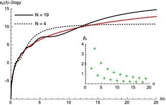
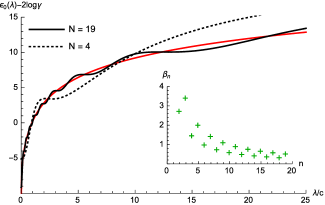
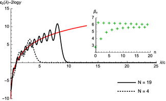
Figure 1: Approximations of $\epsilon_{0}(\lambda)$ (red line) using the transformed cosine (29) (top panel), Chebyshev (31) (middle panel) and Hermite (34) (bottom panel) charges where we have truncated the GGEs to 5 and 20 charges and assuming a finite $c$. For the Chebyshev polynomials the vanishing odd charges are not counted. In the insets of the three panels, the attendant generalized temperatures are plotted.

V.0.1 Alternate Determination of Generalized Temperatures

In Sec. 3 we described a straightforward method of finding the generalized temperatures in the GGE once a system of charges is defined: we expanded the source term, $\epsilon_{0}(\lambda)$, of the generalized free energy on the functions describing the charges in some well defined space of square integrable functions. This process requires knowledge of $\epsilon_{0}(\lambda)$, which may not always be available. In this subsection we will therefore consider an alternative method of finding the generalized temperatures: comparing the expectation values of the charges in the initial state and in a truncated GGE.

In this alternate procedure to determine the generalized temperatures, we suppose that we are given as input the expectation values post-quench of the conserved charges. To then find the generalized temperatures $\beta_{i}$ in $\epsilon_{0}(\lambda)=\sum_{i}\beta_{i}q_{i}(\lambda)$, we will solve the following set of nonlinear equations:

$$\langle\hat{Q}_{i}\rangle=\int\frac{d\lambda}{2\pi}q_{i}(\lambda)\frac{1}{1+e^{\sum_{n=0}^{N}\beta_{n}q_{n}(\lambda)}},\quad i=0,\ldots,N.$$ (93)

Note that solving such a system of nonlinear equations, especially for a large number of generalized temperatures, can be challenging. In fact, we found that the solution is in general not unique and to get the right one we had to use some information available through expanding $\epsilon_{0}(\lambda)$ on $q_{i}(\lambda)$ to set the initial values of the iterative solution scheme. An alternative, more stable method based on exploiting fluctuation-dissipation relations to obtain the generalized temperatures was proposed in Ref. Foini et al. (2017); De Nardis et al. (2017). Assuming for now that we can find the right solution for (93), then to get $\rho_{p}(\lambda)$ we solve Eqs. (20) and (13) consecutively.

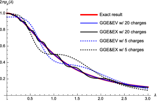
Figure 2: Here are given reconstructions of the mode occupation number density in the $c=\infty$ limit using two different means to determine the generalized temperatures. In the first, labeled GGE&EV, we find the temperatures by performing a fit using Eqn. 93 to the known expectation values of the charges. In the second, labeled GGE&EX, we read off the temperatures by expanding $\epsilon_{0}(\lambda)$ in the basis of charges. Here we compare both methods for two different truncated GGEs: one where we keep the first 5 charges and one where we keep 20. We work with a density of the gas of $n=1/2$ and so the exact rapidity density is given by $\rho_{p}(\lambda)=\frac{1}{2\pi}\frac{1}{1+\lambda^{2}}$ and only $\hat{Q}_{0}$ has a non-vanishing expectation value.

In Fig. 2 we compare reconstructions of the mode occupation density $2\pi\rho_{p}(\lambda)$ in the BEC-to-TG protocol obtained from the two different methods to determine the generalized temperatures for the transformed cosine charges. These two methods are i) truncated expansions of $\epsilon_{0}(\lambda)$ (denoted by ’GGE&EX’) and ii) fitting the parameters of the GGE to the expectation values of charges via Eqn. 93 (termed GGE&EV). We see that when we perform the reconstruction with a small number (5) of charges, the two reconstructions agree (roughly) equally well with the exact form of $\rho_{p}(\lambda)$. However when we expand the number of charges to 20, we see that the GGE&EV method for determining the temperatures leads to almost perfect agreement between $\rho_{p}(\lambda)$ and its reconstruction. However for the GGE&EX method, 20 charges still leads to noticeable deviations.

An important question here is how the temperatures as determined in the GGE&EV method converge to their GGE&EX counterparts as the number of charges in the (truncated) GGE is increased (or whether they converge at all). In Fig. 3 we show the dependence of the first four generalized temperatures on the truncation $N$ obtained in the GGE&EV scheme relative to their GGE&EX values: $\beta_{0}=\beta_{2}=0$, $\beta_{1}=4$, $\beta_{3}=4/3$. The two schemes to determine the generalized temperatures give different reconstructions using the same number of charges, however in the $N\to\infty$ limit the GGE&EV should converge to the GGE&EX values. We however see from Fig. 3 that after a certain $N$ the approach of the two values cease. This happens because when we are solving the nonlinear equations, we have truncated the integral to a finite domain $-50<\lambda<50$ and $-100<\lambda<100$, respectively. We verified that increasing this cutoff starts to slowly decrease the $N\to\infty$ differences between the two methods.

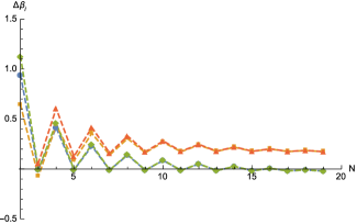
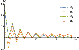
Figure 3: Differences between the GGE&EV values of the first four generalized temperatures for the transformed cosine charges and their GGE&EX values as a function of the truncation $N$. The cutoff in the integral (93) was set $\Lambda=50$ (upper panel) and $\Lambda=100$ (lower panel).

V.0.2 Density-density correlation function from the truncated GGE

As we have indicated, an important measure of how efficient a truncated GGE is its efficacy in describing physical quantities in the post-quench system. To this end we consider the density-density correlation function, both its time independent and time dependent variants.

We begin by looking at the time independent case in the TG limit:

$$G(x)=\langle\rho_{p}|\Phi^{\dagger}(x)\Phi(x)\Phi^{\dagger}(0)\Phi(0)|\rho_{p}\rangle\\ =n^{2}-\left(\int d\lambda e^{ix\lambda}\rho_{p}(\lambda)\right)^{2},$$ (94)

and compare its reconstructions using different truncations of the charges (29). The above formula can easily be proved using (42) De Nardis et al. (2014); Imambekov et al. (2009). (The density-density correlation function can also be obtained in the low energy limit, see Eriksson and Korepin (2013)). In Fig. 4 we show results for the reconstruction of $G(x)$ using 5 and 20 charges whose temperatures are determined in the GGE&EX scheme. In addition to the well-behaving transformed cosine charges (29), we also display results using the Hermite function charges (34) in Fig. 5. Reconstructions in the latter case are far inferior to the former one, as expected.

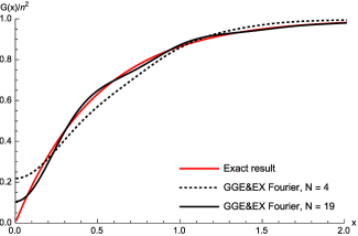
Figure 4: Density-density correlation function in the TG limit at $n=1/2$ from the truncated GGE using 5 and 20 transformed cosine charges.

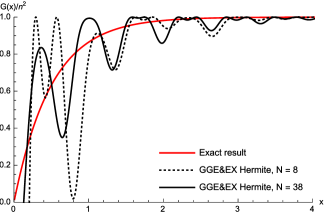
Figure 5: Density-density correlation function in the TG limit at $n=1/2$ from the truncated GGE using 5 and 20 transformed Hermite function charges. (The odd charges with vanishing temperatures are not counted.)

We now turn to the time dependent density-density correlation function or dynamic structure factor (DSF),

$$S(q,\omega)=\int dxdte^{iqx-i\omega t}\langle\rho_{p}|\hat{\rho}(x,t)\hat{\rho}(0,0)|\rho_{p}\rangle,$$ (95)

as obtained from different reconstructions of the representative state. A formula is available for the DSF in the $c\gg 1$ limit (taking here $n=1$) De Nardis and Panfil (2015),

$$S(q,\omega)=\left(\frac{1+6/c}{2q}+\frac{1}{\pi c}\fint d\lambda\frac{n(\lambda+p)-n(\lambda+h)}{\lambda}\right)\\ \times n(h)(1-n(p)),$$ (96)

where $n(\lambda)$ is the filling function, $n(\lambda)=\rho_{p}(\lambda)/(\rho_{p}(\lambda)+\rho_{h}(\lambda))$ and the rapidities $\lambda=p$ and $\lambda=h$ describe the corresponding particle-hole excitation, $q=(1+2/c)(p-h)$ and $\omega=p^{2}-h^{2}$ to first order in $1/c$ or

$$p= \frac{q}{2(1+2/c)}+\frac{\omega(1+2/c)}{2q};$$ (97)

$$h= -\frac{q}{2(1+2/c)}+\frac{\omega(1+2/c)}{2q}.$$ (98)

To exploit the DSF formula at $c$ large, we need to determine the filling function $n(\lambda)$ that corresponds to a truncated GGE. This can be done numerically by expanding $\epsilon_{0}(\lambda)$ in terms of the charges and then solving (20) for $\epsilon=\log(\rho_{h}/\rho_{p})$ – here $\epsilon_{0}(\lambda)$ serves as a source term. Solving this equation is done easily by iteration in Fourier space. The principal value integral in the above expression for $S(q,\omega)$ can easily been evaluated after subtracting the pole contribution at $\lambda=0$, which in any case we found to be heavily suppressed for small $q$. Results of these calculations are shown in Fig. 6.

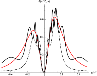
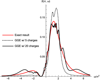
Figure 6: DSF to first order in $1/c$ at $q=\pi/10$ (top panel) and $q=\pi$ (bottom panel) for the representative state after the interaction quench $c=0$ to $c=16$ (red lines) and their approximations using 5 (dotted lines) and 20 charges (black lines) of the transformed cosine charges, $q_{m}(\lambda)=\cos(2m\arctan(\lambda))$.

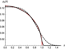
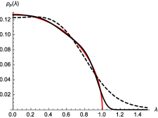
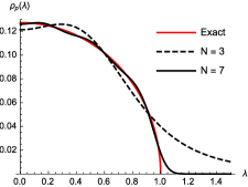
Figure 7: Reconstructions of $\rho_{p}(\lambda)$ for the trap release quench using the ultra-local (left panel), quasi-local Hermite (middle panel) and cosine (right panel) charges using the GGE&EX method at truncations $N=3$ and 7. The parameters of this quench were taken as $n=0.2$ and $\nu=1$.

VI Trap release

While the ultra-local charges are ill-defined for the interaction quench, there are, of course quench protocols where they can be sensibly used. It is interesting in such cases to compare the ultra-local charges with the quasi-local ones to see which perform better. (This is a question that animated Ref. Essler et al. (2017).) We will consider this question in the context of the release of the Lieb-Liniger gas from a harmonic trap. The initial state is the ground state of the Hamiltonian

$$H=-\sum_{j=1}^{N}\frac{\partial^{2}}{\partial x_{j}^{2}}+\frac{1}{4}\sum_{j=1}^{N}\omega^{2}x_{j}^{2}+2c\sum_{i\neq j}\delta(x_{i}-x_{j})$$ (99)

and the dynamics is governed by the Lieb-Liniger Hamiltonian (8), i.e. the above with $\omega=0$. For this quench we will compare the performance of truncated GGEs based on the ultra-local and quasi-local charges.

In Collura et al. (2013a, b) the equilibration of the Tonk-Girardeau gas released from a trap was studied. There the gas was studied in the thermodynamic limit, i.e. $N,L\rightarrow\infty$, with particle density $n=N/L$ fixed, but with the condition that $\nu=\omega N$ was kept constant. They found that $\rho_{p}(\lambda)$ for this quench is given by

$$\rho_{p}(\lambda)=\frac{2n}{\pi\nu}\sqrt{1-(\lambda/\nu)^{2}}$$ (100)

The true tail of $\rho_{p}(\lambda)$ is a Gaussian instead of the sharp cutoff at $\lambda=\nu$ for finite but small $n$. It is clear that this expression only makes sense for $\nu>2^{3/2}n$ (otherwise the filling $2\pi\rho_{p}(\lambda)$ would be greater than 1 near $\lambda=0$). This condition amounts to insisting the size of the gas in its trapped initial state is smaller than the size of the system so that there is an actual expansion of the gas once released.

In order to test which set of charges form a better truncated GGE using the same number of charges, we used the GGE&EX method and solved Eqs. (93) for the transformed cosine, the Hermite, and the ultra-local charges at different truncations. The recovery of the root density is shown in Fig. 7. In this case it is the truncated sets of ultra-local charges that best reproduce the exact $\rho_{p}$.

VII Discussion

We have presented herein a discussion of how one can construct arbitrary bases of conserved charges in integrable models. These bases can be tailored so as to allow them to describe in an efficient manner particular quantum quenches (in the sense that one can write down a GGE density matrix for the post-quench state of the system). One example that we have focused on in this paper is the interaction quench in the Lieb-Liniger model. As we have already discussed, in this quench the standard ultra-local charges fail to describe the quench Kormos et al. (2013); De Nardis et al. (2014). In this quench, excitations are created at arbitrarily high momenta and so only the first three of the ultra-local charges have a finite value after the quench. We however have shown how to construct quasi-local charges that have finite expectation values for this particular quench.

In constructing these quasi-local charges, we do not work directly with operatorial expressions for the charges. Rather we work with the quantity $\epsilon_{0}(\lambda)$, the source term of the pseudo-energy equation in Eqn. 20 (and for the interaction quench given explicitly in Eqn. 25). For our purposes this quantity is primary as it describes the action of the GGE density matrix on a Bethe state $|\{\lambda_{i}\}\rangle$ (where the $\lambda_{i}$’s are solutions to the Bethe equations) via

$$\hat{\rho}_{\text{GGE}}|\{\lambda_{i}\}\rangle=e^{-\sum_{i}\epsilon_{0}(\lambda_{i})}|\{\lambda_{i}\}\rangle.$$ (101)

Thus by expanding the function $\epsilon_{0}(\lambda)$ in terms of a complete set of functions $\{q_{i}(\lambda)\}$, i.e.

$$\epsilon_{0}(\lambda)=\sum_{i}\beta_{i}q_{i}(\lambda),$$ (102)

one can arrive at different sets of charges where the $\beta_{i}$’s are the different inverse temperatures and the $q_{i}(\lambda)$ describe the action of the charges $\hat{Q}_{i}$ on the Bethe states:

$$\hat{Q}_{j}|\{\lambda_{i}\}\rangle=(\sum_{i}q_{j}(\lambda_{i}))|\{\lambda_{i}\}\rangle.$$ (103)

And as we showed in Sections IV, the quasi-locality of the charges is directly correlated with the support of the Fourier transform of $q_{i}(\lambda)$.

The locality property of the sum of all the operators defined in this way, i.e. that of the log of the GGE operator, is controlled however by the locality of $\epsilon_{0}$’s Fourier transform. Equivalently we could inquire about the locality of the charge defined by $\epsilon_{0}$ itself. In case of the interaction quench, the Fourier transform of such a charge has a $1/|x|$ tail, signaling non locality. So while the individual charges that we utilize are always quasi-local, we are actually trying to approximate a non-local operator here. This has been discussed in the context of the different quench, for the XXZ spin-chain model already, in Ilievski et al. (2017); Pozsgay et al. (2017). We note that the non-locality of $\epsilon_{0}$ might have implications for the thermalization of local observables, as we expect that local observables might only thermalize via local GGEs.

One practical advantage of our construction of quasi-local charges over the original ultra-local charges is that we can employ bases of charges, $\{\hat{Q}_{i}\}$ whose action on the Bethe states $\{q_{i}(\lambda)\}$ is bounded in value as the value of $\lambda\rightarrow\infty$. While of course this is necessary if one is to construct a GGE for the interaction quench in Lieb-Liniger, it makes one’s life numerically easier in studying arbitrary quenches. As one example, in Ref. Brandino et al. (2015) a quench of a 1D Bose gas prepared in a parabolic potential and then released into a cosine potential was considered. The aim here was to demonstrate that even though the post-quench Hamiltonian broke integrability, a remnant of the conserved charges survived (at finite particle number). Doing so however was made more difficult by the use of the ultra-local charges. Because the construction used ultra-local charges $Q_{n}$ whose action on a Bethe state was

$$Q_{n}|\{\lambda_{i}\}\rangle=\sum_{i}\lambda^{n}_{i}|\{\lambda_{i}\}\rangle,$$ (104)

one had to deal with charges that took large numerical values. This construction would have been easier if a quasi-local set of operators whose action on the Bethe states was finite had been available at the time.

This work extends the notion of quasi-local charges discussed in Refs. Doyon (2004); Essler et al. (2015, 2017) in the context of the free fermionic field theoretic representation of the quantum Ising model. The discussion here took a different tack than taken there. In Doyon (2004); Essler et al. (2015, 2017), the operatorial expressions of the charges, $I(\alpha)$, were written down first and the corresponding action of the charges then determined. These charges were parameterized by a single positive real variable $\alpha$ controlling their locality (the range of the associated charge density operator equals $\alpha$). Equivalents to these charges do exist in our case for $c=\infty$, the analog being

$$\hat{Q}_{\cos\alpha}|\{\lambda_{i}\}\rangle = \sum_{i}\lambda_{i}^{2}\cos(\alpha\lambda_{i});$$ (105)

$$\hat{Q}_{\sin\alpha}|\{\lambda_{i}\}\rangle = \sum_{i}\sin(\alpha\lambda_{i}).$$ (107)

This is perhaps the most natural basis of expansion of $\epsilon_{0}(\lambda)$, that of a Fourier integral. And these charges have finite expectation values for the interaction quench. Perhaps their only drawback is that this basis is not discrete ($\alpha$ is a continuous variable) and one thus needs a strategy to choose a finite number of them in implementing a truncated GGE (but see Essler et al. (2017) for such a procedure).

Our approach to forming different GGEs includes the particular GGE presented in Ref. Ilievski et al. (2017). In this work the authors advocate forming a GGE density matrix which takes the form (in the context of the Lieb-Liniger model),

$$\hat{\rho}_{\text{GGE}}|\{\lambda_{i}\}\rangle=\frac{1}{\cal Z}\exp\bigg{[}{\int d\lambda\epsilon_{0}(\lambda)\hat{\rho}_{p}(\lambda)}\bigg{]}|\{\lambda_{i}\}\rangle,$$ (108)

exactly the starting point of this paper. Having written $\hat{\rho}_{\text{GGE}}$ in this form, the differences between Ref. Ilievski et al. (2017) and our work begin to appear however. The authors consider their conserved charges in the theory as coming from the operator $\hat{\rho}_{p}(\lambda)$ which acts, in the thermodynamic limit, on a Bethe state, $|\{\lambda_{i}\}\rangle$, via

$$\hat{\rho}_{p}(\lambda)|\{\lambda_{i}\}\rangle=\rho_{p}(\lambda)|\{\lambda_{i}\}\rangle,$$ (109)

i.e. this operator has as its eigenvalues the density of excitations at $\lambda$. This differs from our approach in two ways. We instead treat $\epsilon_{0}\equiv\hat{\epsilon}_{0}$ as an operator, or more precisely a linear combination of quasi-local operators whose coefficients of expansion are the generalized inverse temperatures. The underlying motivation is also different. For Ref. Ilievski et al. (2017), the introduction of $\hat{\rho}_{p}(\lambda)$ as a continuum set of conserved charges is done in the context of a specific model, the XXZ Heisenberg spin chain. There it is known that one needs, in general, to employ not just the ultra-local charges, but an infinite set of families of charges $\{X_{s}(\lambda)\}$, that can be found from a set of generalized transfer matrices built using higher spins, $s$, in the framework of the algebraic Bethe Ansatz. In Ref. Ilievski et al. (2017) it was shown that it was not possible generically to write down a GGE in terms of these charges and so they proposed as an alternative the family of charges, $\{\hat{\rho}_{p}(\lambda)\}$, which while non-local (at least for the case of the Lieb-Liniger – for the XXZ Heisenberg spin chain see the discussion in Ilievski et al. (2017); Pozsgay et al. (2017)), do enable one to write down a GGE for the XXZ Heisenberg model. (We do note parenthetically that if one is willing to represent the GGE as the limit of a set of truncated GGEs, the technical difficulty identified by Ref.Ilievski et al. (2017) is avoided, a fact established in Ref. Pozsgay et al. (2017).) Our motivation is however different. We are interested in finding bases of quasi-local charges that are optimized for different quenches. This is where the practical aspects of our work differs from what was done in Ref. Pozsgay et al. (2017), where $\epsilon_{0}(\lambda)$ was expanded on specific orthogonal linear combinations of a truncated set of specific charges, including the ultra-local ones.

Despite these differences, the finding of Ref. Ilievski et al. (2017) is interesting – namely that there exists complete bases of conserved charges where it is not possible to write down a density matrix involving those charges for an arbitrary quantum quench. It is thus worthwhile asking whether this is the case for Lieb-Liniger model. Here the answer would seem to be no. The problem identified by Ref. Ilievski et al. (2017) could then most likely be associated with a more complicated particle content as the Lieb-Liniger model admits a single particle species. Where such difficulties might show up is any model with string solutions to the Bethe equations (e.g. Piroli et al. (2016a); Vernier and Cubero (2017); Mestyan et al. (2017)), including quenches that involve multi-component Lieb-Liniger systems such as Robinson et al. (2016); Mathy et al. (2012); Gamayun (2014); Burovski et al. (2014).

As we have discussed the findings of Ref. Ilievski et al. (2017), it is worthwhile also to consider a related construction of a set of conserved charges. In the $c=\infty$ limit, an oft used set of charges are associated with the occupation numbers Rigol et al. (2007). The occupation number charges, $\hat{n}_{I}$, have expectation values between 0 and 1 and mark when there is a particle with momentum,

$$\lambda=\frac{2\pi I}{L},$$

where the quantum number $I$ is a half-integer/integer (see Eqn. 11). Using $\epsilon_{0}(\lambda)$ and Eqn. 14 we can generalize this notion away from $c=\infty$. At $c=\infty$ there is a simple relationship between the momenta, $\lambda_{I}$, and the quantum numbers $I$. While at finite $c$, this relationship becomes more complex, it is still possible to write it down as we have done in Eqns. 14 and 15. If $\lambda(I)$ is the momentum determined by the quantum number $I$ as determined by Eqn. 14, the expectation value of the occupation number operator is

$$\langle\hat{n}_{I}\rangle=\frac{1}{1+e^{\epsilon(\lambda(I))}}.$$ (110)

We can easily write the GGE associated with these charges by writing the action of the density matrix on a Bethe state

$$\hat{\rho}_{\text{GGE}}|\{\lambda(I)\}\rangle = \frac{1}{\cal Z}\exp\bigg{[}\sum_{I}\epsilon_{0}(\lambda(I))\bigg{]}|\{\lambda(I)\}\rangle$$ (111)

$$= \frac{1}{\cal Z}\exp\bigg{[}\int dI\frac{\epsilon_{0}(\lambda(I))}{1+e^{\epsilon(\lambda(I))}}\bigg{]}|\{\lambda(I)\}\rangle$$ (113)

$$= \frac{1}{\cal Z}\exp\bigg{[}\int dI\langle\hat{n}_{I}\rangle\epsilon_{0}(\lambda(I))\bigg{]}|\{\lambda(I)\}\rangle.$$ (115)

And so we see that Lagrange multiplier associated with the occupation number operator $\hat{n}_{I}$ is $\epsilon(\lambda(I))$.

While our view of the GGE differs from Ref. Ilievski et al. (2017) with its emphasis on $\rho_{p}(\lambda)$ as the fundamental object, it also differs from one where a microcanonical viewpoint is adopted De Nardis et al. (2017). In the microcanonical viewpoint one often invokes the generalized eigenstate thermalization (gETH) hypothesis. This hypothesis argues that one can employ a representative quantum state, $|s_{\text{rep}}\rangle$, in lieu of performing a trace over a density matrix in computing the expectation value of any reasonable observable O, i.e.

$$\langle s_{\text{rep}}|{\cal O}|s_{\text{rep}}\rangle={\rm Tr}\hat{\rho}_{\text{GGE}}{\cal O}.$$ (117)

In this viewpoint what is important is simply finding a representative state $|s_{\text{rep}}\rangle$. By the gETH, any state that is characterized by an occupation number of excitations given by

$$\frac{\rho_{p}(\lambda)}{\rho_{p}(\lambda)+\rho_{h}(\lambda)}=\frac{1}{1+e^{\epsilon(\lambda)}}$$ (118)

is equally good. And so we see that in this picture it is $\epsilon(\lambda)$ (and not $\epsilon_{0}(\lambda)$) that becomes the primary quantity of interest. Putting aside specific instances where the gETH is known to fail Pozsgay (2014); Goldstein and Andrei (2014), our interest in finding quasi-local bases of charges for quenches mandates that we follow an approach to quantum quenches using a canonical density matrix.

Appendix A

In this appendix we show how to arrive at Eqn. 88 demonstrating that the charges we are constructing are quasi-local at $1/c$. The spatial dependence of the charges is encoded in $F(x_{1},x_{2},x_{3},x_{4})$, defined as:

$$F(x_{1},x_{2},x_{3},x_{4}) =$$ (121)

$$\hskip-101.17755pt\int\frac{d\lambda_{1}}{2\pi}\int\frac{d\lambda_{2}}{2\pi}\int\frac{d\lambda_{3}}{2\pi}C_{\lambda_{1}\lambda_{2}\lambda_{3}}e^{i\lambda_{1}x_{41}}e^{i\lambda_{2}x_{42}}e^{i\lambda_{3}x_{34}}.$$

To evaluate this, we first rewrite $C_{\lambda_{1}\lambda_{2}\lambda_{3}}$ as

$$C_{\lambda_{1}\lambda_{2}\lambda_{3}} = \frac{1}{2}\left[\frac{\lambda_{2}-\lambda_{3}}{\lambda_{1}-\lambda_{3}}-\frac{\lambda_{1}-\lambda_{3}}{\lambda_{2}-\lambda_{3}}\right]$$ (124)

$$\hskip-50.58878pt\times(q(\lambda_{1})+q(\lambda_{2})-q(\lambda_{3})-q(\lambda_{1}+\lambda_{2}-\lambda_{3})).$$

Performing a change of variables, $\{\lambda_{1},\lambda_{2},\lambda_{3}\}\to\{\alpha,\beta,\gamma\}$, with $\alpha=\lambda_{1}-\lambda_{3}$, $\beta=\lambda_{2}-\lambda_{3}$ and $\gamma$ set as the argument of $q$, we can easily evaluate this integral term by term,

$$\frac{1}{2}\int\frac{d\alpha}{2\pi}\int\frac{d\beta}{2\pi}\int\frac{d\gamma}{2\pi}\left(\frac{\beta}{\alpha}-\frac{\alpha}{\beta}\right)q(\gamma)\sum_{i=1}^{4}X_{i}(\alpha,\beta,\gamma).$$ (125)

The exponents $X_{i}$ in the new variables read

$$X_{1}=e^{-i(\alpha x_{32}+\beta x_{24}+\gamma(x_{1}+x_{2}-x_{3}-x_{4}))};$$ (126)

$$X_{2}=e^{-i(\alpha x_{14}+\beta x_{31}+\gamma(x_{1}+x_{2}-x_{3}-x_{4}))};$$ (127)

$$X_{3}=-e^{-i(\alpha x_{14}+\beta x_{24}+\gamma(x_{1}+x_{2}-x_{3}-x_{4}))};$$ (128)

$$X_{4}=-e^{-i(\alpha x_{32}+\beta x_{31}+\gamma(x_{1}+x_{2}-x_{3}-x_{4}))}.$$ (129)

Using

$$\int\frac{d\alpha}{2\pi}\int\frac{d\beta}{2\pi}\frac{\alpha}{\beta}e^{-i\alpha x}e^{-i\beta y}=\frac{1}{2}\delta^{\prime}(x)\text{sgn}(y),$$ (130)

we then obtain our final expression for $F$:

$$F(x_{1},x_{2},x_{3},x_{4}) = \frac{1}{4}\tilde{q}(x_{1}+x_{2}-x_{3}-x_{4})$$ (139)

$$\hskip-57.81621pt\times\bigg{[}(\delta^{\prime}(x_{24})\text{sgn}(x_{32})-\delta^{\prime}(x_{32})\text{sgn}(x_{24}))$$

$$\hskip-50.58878pt+(\delta^{\prime}(x_{31})\text{sgn}(x_{14})-\delta^{\prime}(x_{14})\text{sgn}(x_{31}))$$

$$\hskip-50.58878pt-(\delta^{\prime}(x_{24})\text{sgn}(x_{14})-\delta^{\prime}(x_{14})\text{sgn}(x_{24}))$$

$$\hskip-50.58878pt-(\delta^{\prime}(x_{31})\text{sgn}(x_{32})-\delta^{\prime}(x_{32})\text{sgn}(x_{31}))\bigg{]}.$$

References

- Polkovnikov et al. (2011) A. Polkovnikov, K. Sengupta, A. Silva, and M. Vengalattore, “Colloquium: Nonequilibrium dynamics of closed interacting quantum systems,” Reviews of Modern Physics 83, 863–883 (2011), arXiv:1007.5331 .
- Gogolin and Eisert (2016) C. Gogolin and J. Eisert, “Equilibration, thermalisation, and the emergence of statistical mechanics in closed quantum systems.” Reports on Progress in Physics 79, 056001 (2016), arXiv:1503.07538 .
- Deutsch (1991) J. M. Deutsch, “Quantum statistical mechanics in a closed system,” Physical Review A - Atomic, Molecular, and Optical Physics 43, 2046–2049 (1991), arXiv:1011.1669 .
- Srednicki (1994) M. Srednicki, “Chaos and quantum thermalization,” Physical Review E - Statistical, Nonlinear, and Soft Matter Physics 50, 888–901 (1994), arXiv:cond-mat/9403051 .
- Srednicki (1996) M. Srednicki, “Thermal fluctuations in quantized chaotic systems,” Journal of Physics A: Mathematical and General 29, L75–L79 (1996), arXiv:chao-dyn/9511001 .
- Srednicki (1999) M. Srednicki, “The approach to thermal equilibrium in quantized chaotic systems,” Journal of Physics A: Mathematical and General 32, 1163–1175 (1999), arXiv:cond-mat/9809360 .
- Rigol et al. (2008) M. Rigol, V. Dunjko, and M. Olshanii, “Thermalization and its mechanism for generic isolated quantum systems,” Nature 452, 854–858 (2008), arXiv:0708.1324 .
- Moeckel and Kehrein (2008) M. Moeckel and S. Kehrein, “Interaction Quench in the Hubbard Model,” Physical Review Letters 100, 175702 (2008), arXiv:0802.3202 .
- Rigol and Santos (2010) M. Rigol and L. F. Santos, “Quantum chaos and thermalization in gapped systems,” Physical Review A - Atomic, Molecular, and Optical Physics 82, 011604 (2010), arXiv:1003.1403 .
- Bañuls et al. (2011) M. C. Bañuls, J. I. Cirac, and M. B. Hastings, “Strong and weak thermalization of infinite nonintegrable quantum systems,” Physical Review Letters 106, 050405 (2011), arXiv:1007.3957 .
- Rigol (2014) M. Rigol, “Quantum quenches in the thermodynamic limit,” Physical Review Letters 112, 170601 (2014), arXiv:1401.2160 .
- Rigol et al. (2007) M. Rigol, V. Dunjko, V. Yurovsky, and M. Olshanii, “Relaxation in a completely integrable many-body Quantum system: An Ab initio study of the dynamics of the highly excited states of 1D lattice hard-core bosons,” Physical Review Letters 98, 050405 (2007), arXiv:0604476 .
- Rossini et al. (2009) D. Rossini, A. Silva, G. Mussardo, and G. E. Santoro, “Effective thermal dynamics following a quantum quench in a spin chain,” Physical Review Letters 102, 127204 (2009), arXiv:0810.5508 .
- Rossini et al. (2010) D. Rossini, S. Suzuki, G. Mussardo, G. E. Santoro, and A. Silva, “Long time dynamics following a quench in an integrable quantum spin chain: Local versus nonlocal operators and effective thermal behavior,” Physical Review B - Condensed Matter and Materials Physics 82, 144302 (2010), arXiv:1002.2842 .
- Calabrese et al. (2011) P. Calabrese, F. H. L. Essler, and M. Fagotti, “Quantum Quench in the Transverse Field Ising Chain,” Physical Review Letters 106, 227203 (2011), arXiv:1104.0154 .
- Calabrese et al. (2012a) P. Calabrese, F. H. L. Essler, and M. Fagotti, “Quantum quenches in the transverse field Ising chain: II. Stationary state properties,” Journal of Statistical Mechanics: Theory and Experiment 2012, P07022 (2012a), arXiv:1205.2211 .
- Calabrese et al. (2012b) P. Calabrese, F. H. L. Essler, and M. Fagotti, “Quantum quench in the transverse field Ising chain: I. Time evolution of order parameter correlators,” Journal of Statistical Mechanics: Theory and Experiment 2012, P07016 (2012b), arXiv:1204.3911 .
- Essler et al. (2012) F. H. L. Essler, S. Evangelisti, and M. Fagotti, “Dynamical correlations after a quantum quench,” Physical Review Letters 109, 247206 (2012), arXiv:1208.1961 .
- Mossel and Caux (2010) J. Mossel and J-S. Caux, “Relaxation dynamics in the gapped XXZ spin-1/2 chain,” New Journal of Physics 12, 55028 (2010), arXiv:1002.3988 .
- Mossel and Caux (2012) J. Mossel and J-S. Caux, “Exact time evolution of space- and time-dependent correlation functions after an interaction quench in the one-dimensional Bose gas,” New Journal of Physics 14, 075006 (2012), arXiv:1201.1885 .
- Iucci and Cazalilla (2009) A. Iucci and M. A. Cazalilla, “Quantum quench dynamics of the Luttinger model,” Physical Review A - Atomic, Molecular, and Optical Physics 80, 063619 (2009), arXiv:1003.5170 .
- Dóra et al. (2012) B. Dóra, Á. Bácsi, and G. Zaránd, “Generalized Gibbs ensemble and work statistics of a quenched Luttinger liquid,” Physical Review B - Condensed Matter and Materials Physics 86, 161109 (2012), arXiv:1203.0914 .
- Fioretto and Mussardo (2010) D. Fioretto and G. Mussardo, “Quantum quenches in integrable field theories,” New Journal of Physics 12, 055015 (2010), arXiv:0911.3345 .
- Sotiriadis et al. (2012) S. Sotiriadis, D. Fioretto, and G. Mussardo, “Zamolodchikov-Faddeev algebra and quantum quenches in integrable field theories,” Journal of Statistical Mechanics: Theory and Experiment 2012, P02017 (2012), arXiv:1112.2963 .
- Mussardo (2013) G. Mussardo, “Infinite-Time Average of Local Fields in an Integrable Quantum Field Theory After a Quantum Quench,” Physical Review Letters 111, 100401 (2013), arXiv:1304.7599 .
- Caux and Konik (2012) J-S. Caux and R. M. Konik, “Constructing the Generalized Gibbs Ensemble after a Quantum Quench,” Physical Review Letters 109, 175301 (2012), arXiv:1203.0901 .
- Fagotti et al. (2014) M. Fagotti, M. Collura, F. H.L. Essler, and P. Calabrese, “Relaxation after quantum quenches in the spin-1/2 Heisenberg XXZ chain,” Physical Review B - Condensed Matter and Materials Physics 89, 125101 (2014), arXiv:1311.5216 .
- Pozsgay (2013) B. Pozsgay, “The generalized Gibbs ensemble for Heisenberg spin chains,” Journal of Statistical Mechanics: Theory and Experiment 2013, P07003 (2013), arXiv:1304.5374 .
- Ilievski et al. (2015a) E. Ilievski, J. De Nardis, B. Wouters, J-S. Caux, F. H. L. Essler, and T. Prosen, “Complete Generalized Gibbs Ensembles in an Interacting Theory,” Physical Review Letters 115, 157201 (2015a), arXiv:1507.02993 .
- Essler and Fagotti (2016) F. H. L. Essler and M. Fagotti, “Quench dynamics and relaxation in isolated integrable quantum spin chains,” Journal of Statistical Mechanics: Theory and Experiment 2016, 064002 (2016), arXiv:1603.06452 .
- Vidmar and Rigol (2016) L. Vidmar and M. Rigol, “Generalized Gibbs ensemble in integrable lattice models,” Journal of Statistical Mechanics: Theory and Experiment 2016, 064007 (2016), arXiv:1604.03990 .
- Kormos et al. (2014) M. Kormos, M. Collura, and P. Calabrese, “Analytic results for a quantum quench from free to hard-core one-dimensional bosons,” Physical Review A - Atomic, Molecular, and Optical Physics 89, 013609 (2014), arXiv:1307.2142 .
- Biroli et al. (2010) G. Biroli, C. Kollath, and A. M. Läuchli, “Effect of rare fluctuations on the thermalization of isolated quantum systems,” Physical Review Letters 105, 250401 (2010), arXiv:0907.3731 .
- Gogolin et al. (2011) C. Gogolin, M. P. Muller, and J. Eisert, “Absence of thermalization in nonintegrable systems,” Physical Review Letters 106, 040401 (2011), arXiv:1009.2493 .
- Cazalilla et al. (2012) M. A. Cazalilla, A. Iucci, and M. C. Chung, “Thermalization and quantum correlations in exactly solvable models,” Physical Review E - Statistical, Nonlinear, and Soft Matter Physics 85, 011133 (2012), arXiv:1106.5206 .
- Foini et al. (2012) L. Foini, L. F. Cugliandolo, and A. Gambassi, “Dynamic correlations, fluctuation-dissipation relations, and effective temperatures after a quantum quench of the transverse field Ising chain,” Journal of Statistical Mechanics: Theory and Experiment 2012, P09011 (2012), arXiv:1207.1650 .
- Cassidy et al. (2011) A. C. Cassidy, C. W. Clark, and M. Rigol, “Generalized thermalization in an integrable lattice system,” Physical Review Letters 106, 140405 (2011), arXiv:1008.4794 .
- Pozsgay (2011) B. Pozsgay, “Mean values of local operators in highly excited Bethe states,” Journal of Statistical Mechanics: Theory and Experiment 2011, P01011 (2011), arXiv:1009.4662 .
- Sotiriadis and Calabrese (2014) S. Sotiriadis and P. Calabrese, “Validity of the GGE for quantum quenches from interacting to noninteracting models,” Journal of Statistical Mechanics: Theory and Experiment 2014, 16 (2014), arXiv:1403.7431 .
- Goldstein and Andrei (2014) G. Goldstein and N. Andrei, “Failure of the local generalized Gibbs ensemble for integrable models with bound states,” Physical Review A - Atomic, Molecular, and Optical Physics 90, 043625 (2014), arXiv:1405.4224 .
- Pozsgay et al. (2014) B. Pozsgay, M. Mestyán, M. A. Werner, M. Kormos, G. Zaránd, and G. Takács, “Correlations after Quantum Quenches in the XXZ Spin Chain: Failure of the Generalized Gibbs Ensemble,” Physical Review Letters 113, 117203 (2014), arXiv:1405.2843 .
- Essler et al. (2015) F. H. L. Essler, G. Mussardo, and M. Panfil, “Generalized Gibbs ensembles for quantum field theories,” Physical Review A - Atomic, Molecular, and Optical Physics 91, 051602 (2015), arXiv:1411.5352 .
- Piroli et al. (2016a) L. Piroli, P. Calabrese, and F. H. L. Essler, “Multiparticle Bound-State Formation following a Quantum Quench to the One-Dimensional Bose Gas with Attractive Interactions,” Physical Review Letters 116, 070408 (2016a), arXiv:1509.08234 .
- Bastianello and Sotiriadis (2017) A. Bastianello and S. Sotiriadis, “Quasi locality of the GGE in interacting-to-free quenches in relativistic field theories,” Journal of Statistical Mechanics: Theory and Experiment 2017, P023105 (2017), arXiv:1608.00924 .
- Kormos et al. (2013) M. Kormos, A. Shashi, Y. Zh. Chou, J-S. Caux, and A. Imambekov, “Interaction quenches in the one-dimensional Bose gas,” Physical Review B - Condensed Matter and Materials Physics 88, 205131 (2013), arXiv:1305.7202 .
- Langen et al. (2015) T. Langen, S. Erne, B. Rauer, T. Schweigler, M. Kuhnert, W. Rohringer, T. Gasenzer, and J. Schmiedmayer, “Experimental observation of a generalized Gibbs ensemble,” Science 348, 207–211 (2015), arXiv:1411.7185 .
- Caux and Essler (2013) J-S. Caux and F. H. L. Essler, “Time evolution of local observables after quenching to an integrable model,” Physical Review Letters 110, 257203 (2013), arXiv:1301.3806 .
- Caux (2016) J-S. Caux, “The Quench Action,” Journal of Statistical Mechanics: Theory and Experiment 2016, 064006 (2016), arXiv:1603.04689 .
- De Nardis et al. (2014) J. De Nardis, B. Wouters, M. Brockmann, and J-S. Caux, “Solution for an interaction quench in the Lieb-Liniger Bose gas,” Physical Review A - Atomic, Molecular, and Optical Physics 89, 033601 (2014), arXiv:1308.4310 .
- Wouters et al. (2014) B. Wouters, J. De Nardis, M. Brockmann, D. Fioretto, M. Rigol, and J-S. Caux, “Quenching the anisotropic Heisenberg chain: Exact solution and generalized gibbs ensemble predictions,” Physical Review Letters 113, 117202 (2014), arXiv:1405.0172 .
- Brockmann et al. (2014) M. Brockmann, B. Wouters, D. Fioretto, J. De Nardis, R. Vlijm, and J-S. Caux, “Quench action approach for releasing the Néel state into the spin-1/2 XXZ chain,” Journal of Statistical Mechanics: Theory and Experiment 2014, P12009 (2014), arXiv:1408.5075 .
- Mestyan et al. (2015) M. Mestyan, B. Pozsgay, G. Takacs, and M. A. Werner, “Quenching the XXZ spin chain: quench action approach versus generalized Gibbs ensemble,” Journal of Statistical Mechanics: Theory and Experiment 2015, P04001 (2015), arXiv:1412.4787 .
- Bertini et al. (2017) B. Bertini, E. Tartaglia, and P. Calabrese, “Quantum Quench in the Infinitely Repulsive Hubbard Model: The Stationary State,” Journal of Statistical Mechanics: Theory and Experiment 2017, 103107 (2017), arXiv:1707.01073 .
- Piroli et al. (2016b) L. Piroli, P. Calabrese, and F. H. L. Essler, “Quantum quenches to the attractive one-dimensional Bose gas: exact results,” SciPost Physics 1, 001 (2016b), arXiv:1604.08141 .
- Mestyan et al. (2017) M. Mestyan, B. Bertini, L. Piroli, and P. Calabrese, “Exact solution for the quench dynamics of a nested integrable system,” Journal of Statistical Mechanics: Theory and Experiment 2017, 083103 (2017), arXiv:1705.00851 .
- Bertini et al. (2016) B. Bertini, L. Piroli, and P. Calabrese, “Quantum quenches in the sinh-gordon model: steady state and one-point correlation functions,” Journal of Statistical Mechanics: Theory and Experiment 2016, 063102 (2016), arXiv:1602.08269 .
- D’Alessio et al. (2016) L. D’Alessio, Y. Kafri, A. Polkovnikov, and M. Rigol, “From Quantum Chaos and Eigenstate Thermalization to Statistical Mechanics and Thermodynamics,” Advances in Physics 65, 239 (2016), arXiv:1509.06411 .
- Alba and Calabrese (2017) V. Alba and P. Calabrese, “Quench action and Renyi entropies in integrable systems,” Physical Review B - Condensed Matter and Materials Physics 96, 115421 (2017), arXiv:1705.10765 .
- Piroli et al. (2016c) L. Piroli, E. Vernier, and P. Calabrese, “Exact steady states for quantum quenches in integrable heisenberg spin chains,” Physical Review B - Condensed Matter and Materials Physics 94, 054313 (2016c), arXiv:1606.00383 .
- Ilievski et al. (2016a) E. Ilievski, E. Quinn, J. De Nardis, and M. Brockmann, “String-charge duality in integrable lattice models,” Journal of Statistical Mechanics: Theory and Experiment 2016, 063101 (2016a), arXiv:1512.04454 .
- Essler et al. (2017) F. H. L. Essler, G. Mussardo, and M. Panfil, “On truncated generalized Gibbs ensembles in the Ising field theory,” Journal of Statistical Mechanics: Theory and Experiment 2017, 013103 (2017), arXiv:1610.02495 .
- Lieb and Liniger (1963) E. H. Lieb and W. Liniger, “Exact Analysis of an Interacting Bose Gas. I. The General Solution and the Ground State,” Physical Review 130, 1605 (1963).
- Lieb (1963) E. H. Lieb, “Exact Analysis of an Interacting Bose Gas. II. The Excitation Spectrum,” Physical Review 130, 1616 (1963).
- Ilievski et al. (2015b) E. Ilievski, M. Medenjak, and T. Prosen, “Quasilocal conserved operators in the isotropic heisenberg spin- chain,” Phys. Rev. Lett. 115, 120601 (2015b), arXiv:1506.05049 .
- Ilievski et al. (2016b) E. Ilievski, M. Medenjak, T. Prosen, and L. Zadnik, “Quasilocal charges in integrable lattice systems,” Journal of Statistical Mechanics: Theory and Experiment 2016, 064008 (2016b), arXiv:1603.00440 .
- Ilievski et al. (2017) E. Ilievski, E. Quinn, and J-S. Caux, “From interacting particles to equilibrium statistical ensembles,” Physical Review B - Condensed Matter and Materials Physics 95, 115128 (2017), arXiv:1610.06911 .
- Pozsgay et al. (2017) B. Pozsgay, E. Vernier, and M. Werner, “On Generalized Gibbs Ensembles with an infinite set of conserved charges,” Journal of Statistical Physics: Theory and Experiment 2017, 093103 (2017), arXiv:1703.09516 .
- Korepin et al. (1993) V. E. Korepin, N. M. Bogoliubov, and A. G. Izergin, Quantum inverse scattering method and correlation functions (Cambridge University Press, Cambridge, 1993).
- James et al. (2017) A. J. A. James, R. M. Konik, P. Lecheminant, N. J. Robinson, and A. M. Tsvelik, “Non-perturbative methodologies for low-dimensional strongly-correlated systems: From non-Abelian bosonization to truncated spectrum methods,” Reports on Progress in Physics (2017), arXiv:1703.08421 .
- Fagotti (2016) M. Fagotti, “Local conservation laws in spin-1/2 XY chains with open boundary conditions,” Journal of Statistical Mechanics: Theory and Experiment 2016, P063105 (2016), arXiv:1601.02011 .
- Erdelyi (1955) A. Erdelyi, “Asymptotic Representations of Fourier Integrals and the Method of Stationary Phase,” Journal of the Society for Industrial and Applied Mathematics 3, 17–27 (1955).
- Davies (1990) B. Davies, “Higher conservation laws for the quantum non-linear Schrodinger equation,” Physica A: Statistical Mechanics and its Applications 167, 433–456 (1990), arXiv:1109.6604 .
- Davies and Korepin (2011) B. Davies and V. E. Korepin, “Higher conservation laws for the quantum non-linear Schroedinger equation,” ArXiv e-prints (2011), arXiv:1109.6604 .
- Cheon and Shigehara (1999) T. Cheon and T. Shigehara, “Fermion-Boson Duality of One-Dimensional Quantum Particles with Generalized Contact Interactions,” Physical Review Letters 82, 2536–2539 (1999), arXiv:quant-ph/9806041 .
- Yukalov and Girardeau (2005) V. I. Yukalov and M. D. Girardeau, “Fermi-Bose mapping for one-dimensional Bose gases,” Laser Physics Letters 2, 375–382 (2005), arXiv:cond-mat/0507409 .
- Khodas et al. (2007) M. Khodas, M. Pustilnik, A. Kamenev, and L. I. Glazman, “Dynamics of excitations in a one-dimensional bose liquid,” Physical Review Letters 99, 110405 (2007), arXiv:0705.2015 .
- Brand and Cherny (2005) J. Brand and A. Yu. Cherny, “Dynamic structure factor of the one-dimensional Bose gas near the Tonks-Girardeau limit,” Physical Review A - Atomic, Molecular, and Optical Physics 72, 033619 (2005), arXiv:0410311 .
- Cherny and Brand (2006) A. Yu. Cherny and J. Brand, “Polarizability and dynamic structure factor of the one-dimensional Bose gas near the Tonks-Girardeau limit at finite temperatures,” Physical Review A - Atomic, Molecular, and Optical Physics 73, 023612 (2006), arXiv:0507086 .
- Foini et al. (2017) L. Foini, A. Gambassi, R. Konik, and L. F. Cugliandolo, “Measuring effective temperatures in a generalized Gibbs ensemble,” Physical Review E - Statistical, Nonlinear, and Soft Matter Physics 95, 052116 (2017), arXiv:1610.00101 .
- De Nardis et al. (2017) J. De Nardis, M. Panfil, A. Gambassi, L. F. Cugliandolo, R. Konik, and L. Foini, “Probing non-thermal density fluctuations in the one-dimensional Bose gas,” SciPost Physics 3, 023 (2017), arXiv:1704.06649 .
- Imambekov et al. (2009) A. Imambekov, I. E. Mazets, D. S. Petrov, V. Gritsev, S. Manz, S. Hofferberth, T. Schumm, E. Demler, and J. Schmiedmayer, “Density ripples in expanding low-dimensional gases as a probe of correlations,” Physical Review A - Atomic, Molecular, and Optical Physics 80, 033604 (2009), arXiv:0904.1723 .
- Eriksson and Korepin (2013) Erik Eriksson and Vladimir Korepin, “Finite-size effects from higher conservation laws for the one-dimensional bose gas,” Journal of Physics A: Mathematical and Theoretical 46, 235002 (2013).
- De Nardis and Panfil (2015) J. De Nardis and M. Panfil, “Density form factors of the 1D Bose gas for finite entropy states,” Journal of Statistical Mechanics: Theory and Experiment 2015, P02019 (2015), arXiv:1411.4537 .
- Collura et al. (2013a) M. Collura, S. Sotiriadis, and P. Calabrese, “Equilibration of a Tonks-Girardeau gas following a trap release,” Physical Review Letters 110, 245301 (2013a), arXiv:1303.3795 .
- Collura et al. (2013b) M. Collura, S. Sotiriadis, and P. Calabrese, “Quench dynamics of a Tonks-Girardeau gas released from a harmonic trap,” Journal of Statistical Mechanics: Theory and Experiment 2013, 52 (2013b), arXiv:1306.5604 .
- Brandino et al. (2015) G. P. Brandino, J.-S. Caux, and R. M. Konik, “Glimmers of a Quantum KAM Theorem: Insights from Quantum Quenches in One-Dimensional Bose Gases,” Physical Review X 5, 041043 (2015), arXiv:1407.7167 .
- Doyon (2004) B. Doyon, Correlation Functions in Integrable Quantum Field Theory, Ph.D. thesis, Rutgers University (2004).
- Vernier and Cubero (2017) E. Vernier and A. C. Cubero, “Quasilocal charges and progress towards the complete GGE for field theories with nondiagonal scattering,” Journal of Statistical Mechanics: Theory and Experiment 2017, 023101 (2017), arXiv:1609.03220 .
- Robinson et al. (2016) N. J. Robinson, J-S. Caux, and R. M. Konik, “Motion of a Distinguishable Impurity in the Bose Gas: Arrested Expansion Without a Lattice and Impurity Snaking,” Physical Review Letters 116, 145302 (2016), arXiv:1506.03502 .
- Mathy et al. (2012) C. J. M. Mathy, M. B. Zvonarev, and E. Demler, “Quantum flutter of supersonic particles in one-dimensional quantum liquids,” Nature Physics 8, 881–886 (2012), arXiv:1203.4819 .
- Gamayun (2014) O. Gamayun, “Quantum Boltzmann equation for a mobile impurity in a degenerate Tonks-Girardeau gas,” Physical Review A - Atomic, Molecular, and Optical Physics 89, 063627 (2014), arXiv:1402.7064 .
- Burovski et al. (2014) E. Burovski, V. Cheianov, O. Gamayun, and O. Lychkovskiy, “Momentum relaxation of a mobile impurity in a one-dimensional quantum gas,” Physical Review A - Atomic, Molecular, and Optical Physics 89, 041601 (2014), arXiv:1308.6147 .
- Pozsgay (2014) B. Pozsgay, “Failure of the generalized eigenstate thermalization hypothesis in integrable models with multiple particle species,” Journal of Statistical Mechanics: Theory and Experiment 2014, P09026 (2014), arXiv:1406.4613 .