Uniform analytic approximation of Wigner rotation matrices

Abstract

We derive the leading asymptotic approximation, for low angle $\theta$, of the Wigner rotation matrix elements $d_{m_{1}m_{2}}^{j}(\theta)$, uniform in $j,m_{1}$ and $m_{2}.$ The result is in terms of a Bessel function of integer order. We numerically investigate the error for a variety of cases and find that the approximation can be useful over a significant range of angles. This approximation has application in the partial wave analysis of wavepacket scattering.

I Introduction

The purpose of this paper is to derive an approximation for the Wigner rotation matrices, $d_{m_{1}m_{2}}^{j}(\theta)$, as a function of the angle $\theta$ and uniform in $j,m_{1}$ and $m_{2},$ for use in analytic calculations.

There are several methods available for computing individual Wigner rotation matrix elements to high precision. Wigner’s series for the matrix elements (equivalent to the terminating hypergeometric series in Eq. (II.1) below) becomes, for large indices, a sum of very large terms with alternating signs, exceeding the floating-point precision. One of the alternative methods involves using recurrence relations obeyed by the matrix elements Dachsel (2006); Choi et al. (1999). A precision of 15 significant figures can be obtained. Another method involves converting the sum into a Fourier series, which is better behaved Feng et al. (2015); Tajima (2015). Fukushima Fukushima (2016) presents a method, using recurrence relations and extension of floating-point exponents that can achieve 16 significant figures for very large values of the indices.

The approximation presented here cannot obtain the very high precisions of the methods just mentioned, as we will see below. However, it has the advantage of giving the approximation as a function of the angle, which can then be used in integrals.

The motivation for this work came from a recent paper by the author Hoffmann (2017) on the scattering theory of wavepackets in a Coulomb potential. The system considered was a single, nonrelativistic, spinless particle, but the results presented here should have wider applicability: to multiple particles, nonvanishing spins and relativistic treatments Jacob and Wick (1959); Macfarlane (1962).

It was necessary to transform the wavefunction from a basis of momentum eigenvectors (with wavefunction $\Psi_{\mathrm{0}}(\boldsymbol{k})$) to a basis of free eigenvectors of the magnitude of momentum, $k$, and the familiar angular momentum quantum numbers, $l$ and $m$, taking only integer values in this case (with wavefunction $\Psi(k,l,m)$). The transformation is

$$\Psi(k,l,m)=k\int_{0}^{\pi}\sin\theta\,d\theta\int_{0}^{2\pi}d\varphi\,Y_{lm}^{*}(\theta,\varphi)\Psi_{\mathrm{0}}(\boldsymbol{k}),$$ (I.1)

where $k=|\boldsymbol{k}|$ and $\hat{k}$ has spherical polar coordinates $(\theta,\varphi)$.

To illustrate the method and avoid complications regarding wavepacket spreading, we choose the simple, normalized momentum wavefunction

$$\Psi_{0}(\boldsymbol{k})=\frac{e^{-|\boldsymbol{k}-p\hat{\boldsymbol{z}}|^{2}/4\sigma_{p}^{2}}}{(2\pi\sigma_{p}^{2})^{\frac{3}{4}}}.$$ (I.2)

The following calculation is simplest if the average momentum is chosen in the $z$ direction. The standard deviation of each momentum component is $\sigma_{p}.$

In a scattering experiment, we want the initial momentum to be well resolved, so we choose

$$\epsilon\equiv\frac{\sigma_{p}}{p}\ll 1.$$ (I.3)

The results we derive below will be to lowest order in $\epsilon.$ It is the small magnitude of this parameter that will allow us to construct an approximation method for which the leading term will be sufficient for our purposes.

The spherical harmonic can be expressed in terms of a Wigner rotation matrix as

$$Y_{lm}^{*}(\theta,\varphi)=\sqrt{\frac{2l+1}{4\pi}}e^{-im\varphi}d_{m0}^{l}(\theta),$$ (I.4)

so

$$\int_{0}^{2\pi}d\varphi\,e^{-im\varphi}=2\pi\,\delta_{m0}.$$ (I.5)

Then we use

$$|\boldsymbol{k}-p\hat{\boldsymbol{z}}|^{2}=(k-p)^{2}+2kp(1-\cos\theta).$$ (I.6)

So the remaining integral for the wavefunction becomes

$$\Psi(k,l,m)=\delta_{m0}\sqrt{2\pi}\,k\,e^{-(k-p)^{2}/4\sigma_{p}^{2}}\sqrt{l+\frac{1}{2}}\int_{0}^{\pi}\sin\theta\,d\theta\,e^{-kp(1-\cos\theta)/2\sigma_{p}^{2}}d_{00}^{l}(\theta).$$ (I.7)

It was intended to find an analytic approximation to this integral, so that we could make contact with results from partial wave analysis and to minimize the amount of numerical computation needed. The final calculation of the differential cross section then requires only a numerical evaluation of a sum over $l$ Hoffmann (2017).

In Eq. (I.7) the Gaussian in $k$ is only significant for $k=p+\mathcal{O}(\sigma_{p})$. Then the exponential function of $\theta$ is sharply peaked at $\theta=0$ with a width of order $\epsilon.$ To evaluate this integral, we cannot use a Taylor series for the rotation matrix, as for large $l$ it oscillates many times within the peak of the exponential. Instead, we need an approximation valid for low $\theta$ that is uniform in $l$. We use the method of Olver Olver (1974) for obtaining such expansions from the differential equation for the function.

The Wigner rotation matrices are matrix elements of unitary rotations about the $y$ axis,

$$d_{m_{1}m_{2}}^{j}(\theta)=\langle\,j,m_{1}\,|\,e^{-i\theta J_{y}}\,|\,j,m_{2}\,\rangle,$$ (I.8)

and with the Condon-Shortley phase convention Messiah (1961) the matrix elements are all real.

The Wigner rotation matrices are predefined functions in MATHEMATICA (WignerD) Mat (2017). Note that the MATHEMATICA sign convention is

$$\mathtt{WignerD}[\{j,m_{1},m_{2}\},\theta]=d_{-m_{1},-m_{2}}^{j}(\theta).$$ (I.9)

Note that in other cases of interest Jacob and Wick (1959); Macfarlane (1962), more general rotation matrices $d_{m_{1}m_{2}}^{j}(\theta)$ will appear in place of

$$d_{00}^{l}(\theta)=P_{l}(\cos\theta),$$ (I.10)

including for half-integral angular momentum. We will derive a result valid for the general case.

II Asymptotic approximation from the differential equation

Wigner’s series for the rotation matrix elements $d_{m_{1}m_{2}}^{j}(\theta)$ can be written in terms of a terminating hypergeometric series as Rose (1957)

$$d_{m_{1}m_{2}}^{j}(\theta)=\left[\frac{(j+m_{1})!(j-m_{2})!}{(j-m_{1})!(j+m_{2})!}\right]^{\frac{1}{2}}\frac{(-)^{m_{1}-m_{2}}}{(m_{1}-m_{2})!}(\sin\frac{\theta}{2})^{m_{1}-m_{2}}(\cos\frac{\theta}{2})^{2j+m_{2}-m_{1}}\times\\ \times\phantom{|}_{2}F_{1}(-(j-m_{1}),-(j+m_{2});m_{1}-m_{2}+1;-\tan^{2}\frac{\theta}{2})$$ (II.1)

for $m_{1}\geq m_{2}.$ We consider this regime first, then, for $m_{1}\leq m_{2},$ we use the symmetry relation Messiah (1961)

$$d_{m_{1}m_{2}}^{j}(\theta)=(-)^{m_{1}-m_{2}}d_{m_{2}m_{1}}^{j}(\theta).$$ (II.2)

This form gives us the small $\theta$ behaviour (again for $m_{1}\geq m_{2}$)

$$d_{m_{1}m_{2}}^{j}(\theta)\sim\left[\frac{(j+m_{1})!(j-m_{2})!}{(j-m_{1})!(j+m_{2})!}\right]^{\frac{1}{2}}\frac{(-)^{m_{1}-m_{2}}}{(m_{1}-m_{2})!}(\frac{\theta}{2})^{m_{1}-m_{2}},$$ (II.3)

which we will use shortly.

An equivalent form is in terms of a Jacobi polynomial Szegö (1939)

$$d_{m_{1}m_{2}}^{j}(\theta)=(-)^{m_{1}-m_{2}}\left[\frac{(j+m_{1})!(j-m_{1})!}{(j+m_{2})!(j-m_{2})!}\right]^{\frac{1}{2}}(\sin\frac{\theta}{2})^{m_{1}-m_{2}}(\cos\frac{\theta}{2})^{m_{1}+m_{2}}\times\\ \times P_{j-m_{1}}^{(m_{1}-m_{2},m_{1}+m_{2})}(\cos\theta).$$ (II.4)

The function

$$w(\theta)=(\sin\frac{\theta}{2}\cos\frac{\theta}{2})^{\frac{1}{2}}d_{m_{1}m_{2}}^{j}(\theta)$$ (II.5)

obeys the particularly simple differential equation Abramowitz and Stegun (1972)

$$\{\frac{d^{2}}{d\theta^{2}}+(j+\frac{1}{2})^{2}-\frac{\alpha^{2}-\frac{1}{4}}{4\sin^{2}\frac{\theta}{2}}-\frac{\beta^{2}-\frac{1}{4}}{4\cos^{2}\frac{\theta}{2}}\}w=0,$$ (II.6)

with

$$\alpha \equiv m_{1}-m_{2},$$ (II.7)

$$\beta \equiv m_{1}+m_{2}.$$ (II.8)

Since we are looking for a low angle approximation, we expand the trigonometric factors in powers of $\theta,$ keeping terms of order $\theta^{2}$ in the differential equation. This gives the approximate equation

$$\{\frac{d^{2}}{d\theta^{2}}+\Delta^{2}-\frac{\alpha^{2}-\frac{1}{4}}{\theta^{2}}+\psi(\theta)\}w=0,$$ (II.9)

where

$$\Delta(j,m_{1},m_{2})\equiv\sqrt{j(j+1)-\frac{1}{3}(m_{1}^{2}+m_{2}^{2}+m_{1}m_{2}-1)}$$ (II.10)

and

$$\psi(\theta)\sim\frac{(\alpha^{2}-\frac{1}{4})}{\Delta^{2}}\frac{\theta^{2}}{160}-\frac{(\beta^{2}-\frac{1}{4})}{\Delta^{2}}\frac{\theta^{2}}{16}$$ (II.11)

for small $\theta.$ Note that

$$j(j+1)-\frac{1}{3}(m_{1}^{2}+m_{2}^{2}+m_{1}m_{2}-1)\geq j+\frac{1}{3}$$ (II.12)

for given $j,$ so is always strictly positive.

Now we define

$$z\equiv\Delta\theta$$ (II.13)

and use the transformation

$$w=\sqrt{z}\,y(z).$$ (II.14)

Then the differential equation becomes

$$\{\frac{d^{2}}{dz^{2}}+\frac{1}{z}\frac{d}{dz}+1-\frac{\alpha^{2}}{z^{2}}+\psi(\frac{z}{\Delta})\}y=0.$$ (II.15)

If the correction factor, $\psi(\theta),$ is sufficiently small and can be neglected, this becomes the differential equation for the Bessel function Gradsteyn and Ryzhik (1980) (the solution finite at the origin)

$$y(z)=J_{\alpha}(z).$$ (II.16)

Instead of analytically calculating bounds on the error in our approximation, we use numerical methods in Section III.

Now we have

$$w(\theta)\sim C\,\theta^{\frac{1}{2}}J_{m_{1}-m_{2}}(\Delta\theta),$$ (II.17)

which then gives

$$d_{m_{1}m_{2}}^{j}(\theta)\sim D(\frac{\theta}{\sin\theta})^{\frac{1}{2}}J_{m_{1}-m_{2}}(\Delta\theta)$$ (II.18)

for $m_{1}\geq m_{2}.$

To normalize the solutions, we note

$$J_{m_{1}-m_{2}}(\Delta\theta)\cong\frac{1}{(m_{1}-m_{2})!}(\Delta\frac{\theta}{2})^{m_{1}-m_{2}}$$ (II.19)

for small $\theta.$ Comparing with Eq. (II.3), we find

$$D(j,m_{1},m_{2})=(-)^{m_{1}-m_{2}}\left[\frac{(j+m_{1})!(j-m_{2})!}{(j-m_{1})!(j+m_{2})!}\right]^{\frac{1}{2}}\frac{1}{\Delta^{m_{1}-m_{2}}}.$$ (II.20)

Finally

$$d_{m_{1}m_{2}}^{j}(\theta)=(-)^{m_{1}-m_{2}}\left[\frac{(j+m_{1})!(j-m_{2})!}{(j-m_{1})!(j+m_{2})!}\right]^{\frac{1}{2}}\frac{1}{\Delta(j,m_{1},m_{2})^{m_{1}-m_{2}}}\times\\ \times(\frac{\theta}{\sin\theta})^{\frac{1}{2}}J_{m_{1}-m_{2}}(\Delta(j,m_{1},m_{2})\theta)+\mathcal{E}(j,m_{1},m_{2},\theta).$$ (II.21)

for $m_{1}\geq m_{2}.$ We will find numerical bounds on the absolute error, $|\mathcal{E}(j,m_{1},m_{2},\theta)|$, in the next section. Note that

$$|d_{m_{1}m_{2}}^{j}(\theta)|\leq 1$$ (II.22)

from unitarity.

Note also that in typical applications we have

$$j\gg|m_{1}|,|m_{2}|,$$ (II.23)

in which case

$$\left[\frac{(j+m_{1})!(j-m_{2})!}{(j-m_{1})!(j+m_{2})!}\right]^{\frac{1}{2}}\frac{1}{\Delta(j,m_{1},m_{2})^{m_{1}-m_{2}}}=1+\mathcal{O}(\frac{m_{i}}{j})\quad i=1,2.$$ (II.24)

III Numerical calculation of error bounds

In the applications we envision, for example the scattering of two particles, $m_{2}$ will be a difference of helicities, not a large number. For an impact parameter of, say, $10\,\sigma_{x}$, where $\sigma_{x}=1/2\sigma_{p},$ we expect the wavefunction to only be significant for $m_{1}\apprle 10.$ Furthermore, for a typical choice, $\epsilon=0.001$, the wavefunction will only be significant for $j\apprle 2\,000.$

We first try a simple example that will be relevant to our original problem, finding the error bound for

$$d_{00}^{j}(\theta)=P_{j}(\cos\theta)=(\frac{\theta}{\sin\theta})^{\frac{1}{2}}J_{0}(\sqrt{j(j+1)+\frac{1}{3}}\,\theta)+\mathcal{E}(j,\theta).$$ (III.1)

We plot the absolute error, $|\mathcal{E}(j,\theta)|$, and $|P_{j}(\cos\theta)|$ (as calculated by MATHEMATICA) against $\theta$ on log-log plots for (a) $j=10$ and (b) $j=2\,000$ in Figure 1.

As expected, we see the absolute and relative errors rising with angle. For the small angles, $\theta\sim\epsilon$ that dominate the integral Eq. (I.7), the relative error remains less than about $10^{-6}$ over the range of physical $j$ values. We plot the dependence on $j$ for $\theta=0.001$ explicitly in Figure 2, confirming these conclusions.

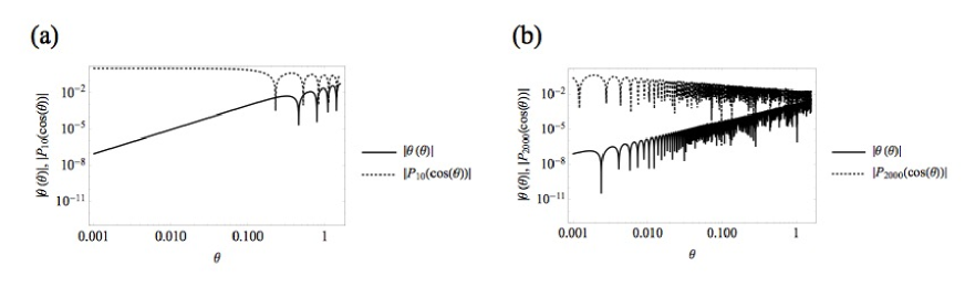
Figure 1: Absolute errors for our approximation of $d_{00}^{j}(\theta)$, compared to $|P_{j}(\cos\theta)|$ for (a) $j=10$ and (b) $j=2\,000.$

Figure 2: Absolute errors for our approximation of $d_{00}^{j}(0.001)$, compared to $|P_{j}(\cos 0.001)|$ for the physical range of $j.$

At another extreme, to see a case where our approximation may be less valid, we investigate

$$d_{jj}^{j}(\theta)=(\frac{\theta}{\sin\theta})^{\frac{1}{2}}J_{0}(\sqrt{j+\frac{1}{3}}\,\theta)\{1+\mathcal{R}(j,\theta)\},$$ (III.2)

using MATHEMATICA for the exact Wigner matrices. For this example we plot the relative errors, defined by

$$\mathcal{R}(j,\theta)=\{d_{jj}^{j}(\theta)-(\frac{\theta}{\sin\theta})^{\frac{1}{2}}J_{0}(\sqrt{j+\frac{1}{3}}\,\theta)\}/d_{jj}^{j}(\theta),$$ (III.3)

in Figure 3. We see again that the error rises with angle, and it also increases with $j.$ For the low angle $\theta=\epsilon$, the relative error is less than $10^{-7}$ for $j=2000.$

Figure 3: Relative errors for our approximation of $d_{jj}^{j}(\theta)$, for $j=0,20,200,2000.$

We conclude with an example using half-integer spins,

$$d_{\frac{5}{2},\frac{1}{2}}^{j}(\theta)=\left[\frac{(j+\frac{5}{2})!(j-\frac{1}{2})!}{(j-\frac{5}{2})!(j+\frac{1}{2})!}\right]^{\frac{1}{2}}\frac{1}{j(j+1)-\frac{9}{4}}(\frac{\theta}{\sin\theta})^{\frac{1}{2}}J_{2}(\sqrt{j(j+1)-\frac{9}{4}}\,\theta)+\mathcal{E}(j,\theta)$$ (III.4)

for $j\geq\frac{5}{2}$. The absolute error and $|d_{\frac{5}{2},\frac{1}{2}}^{j}(\theta)|$ (MATHEMATICA) are plotted in Figure 4 for $j=2000.5$. Again we find very small relative errors at low angles, rising with angle.

Figure 4: Absolute error for our approximation of $d_{\frac{5}{2},\frac{1}{2}}^{2000.5}(\theta)$.

IV Approximation of the integral

Returning to our original problem, we consider the factor from Eq. (I.7) (with $\rho=k/p$)

$$I(\rho,l)=\frac{1}{2\epsilon^{2}}\int_{0}^{\pi}\sin\theta\,d\theta\,e^{-\rho(1-\cos\theta)/2\epsilon^{2}}P_{l}(\cos\theta).$$ (IV.1)

We make the further approximations $\sin\theta=\theta(1+\mathcal{O}(\theta^{2}))$ and $1-\cos\theta=\frac{\theta^{2}}{2}(1+\mathcal{O}(\theta^{2}))$ in the exponent and extend the upper limit of the integral to infinity to find Gradsteyn and Ryzhik (1980)

$$I(\rho,l) \sim \frac{1}{2\epsilon^{2}}\int_{0}^{\infty}\theta\,d\theta\,e^{-\rho\theta^{2}/4\epsilon^{2}}J_{0}(\sqrt{l(l+1)+\frac{1}{3}}\,\theta)$$ (IV.2)

$$= \frac{1}{\rho}e^{-\epsilon^{2}(l(l+1)+\frac{1}{3})/\rho}$$

to lowest order in $\epsilon=\sigma_{p}/p$. A narrow distribution in angle produces a wide distribution in angular momentum.

We define the relative error in this approximation as

$$\mathcal{R}(\rho,l)=\{I(\rho,l)-\frac{1}{\rho}e^{-\epsilon^{2}(l(l+1)+\frac{1}{3})/\rho}\}/I(\rho,l).$$ (IV.3)

In Figure 5 we plot the magnitude of this relative error for $\rho=1$ as a function of $l,$ up to three standard deviations. We see that the relative error is $\apprle 10^{-5}.$ The dependence on $\rho$ is very gradual, with the relative error changing by only $7\,\%$ of its $\rho=1$ value over $|\rho-1|\leq 10\,\epsilon$ for $l=3000.$

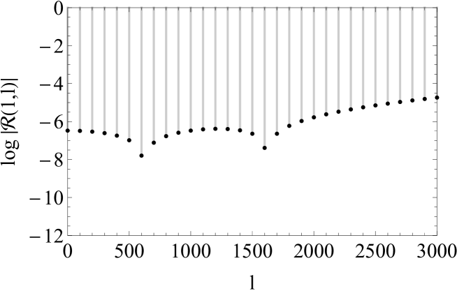
Figure 5: Relative error for $\rho=1.$

V Conclusions

We have found a low angle approximation of the Wigner rotation matrix elements, $d_{m_{1}m_{2}}^{j}(\theta)$, uniform in $j,m_{1}$ and $m_{2}.$ Numerical determinations of errors in this approximation have been given for a variety of cases. The relative error is reduced if $j\gg|m_{1}|,|m_{2}|,$ which is the case in the applications we envision. For our original problem of approximating a change of basis, our method gives a relative error of $10^{-5}.$ We expect that this approximation will have applications in the partial wave analysis of wavepacket scattering.

The approximation presented here is merely the leading approximate solution of a differential equation in the low angle region. It is possible that an approximation with greater precision can be produced by calculating additional terms.

References

• Dachsel (2006) H. Dachsel, J. Chem. Phys. 124, 144115 (2006).
• Choi et al. (1999) C. H. Choi, J. Ivanic, M. S. Gordon,  and K. Ruedenberg, J. Chem. Phys. 111, 8825 (1999).
• Feng et al. (2015) X. M. Feng, P. Wang, W. Yang,  and G. R. Jin, Phys. Rev. E 92, 043307 (2015).
• Tajima (2015) N. Tajima, Phys. Rev. C 91, 014320 (2015).
• Fukushima (2016) T. Fukushima, Numerical computation of Wigner’s d-function of arbitrary high degree and orders by extending exponent of floating point numbers, Tech. Rep. (National Astronomical Observatory of Japan, 2016).
• Hoffmann (2017) S. E. Hoffmann, J. Phys. B: At. Mol. Opt. Phys. 50, 215302 (2017).
• Jacob and Wick (1959) M. Jacob and G. C. Wick, Ann. of Phys. (N.Y.) 7, 404 (1959).
• Macfarlane (1962) A. J. Macfarlane, Rev. Mod. Phys. 34, 41 (1962).
• Olver (1974) F. W. J. Olver, Asymptotics and Special Functions (Academic Press, N.Y., 1974).
• Messiah (1961) A. Messiah, Quantum Mechanics, Vol. 1 and 2 (North-Holland, Amsterdam and John Wiley and Sons, N.Y., 1961).
• Mat (2017) “Wolfram Research Inc. Mathematica,” https://www.wolfram.com (2017).
• Rose (1957) M. E. Rose, Elementary Theory of Angular Momentum (John Wiley and Sons, Inc., N. Y., 1957).
• Szegö (1939) G. Szegö, Orthogonal Polynomials (A.M.S., Providence, R.I., 1939).
• Abramowitz and Stegun (1972) M. Abramowitz and I. A. Stegun, Handbook of Mathematical Functions, 9th ed. (Dover, N. Y., 1972).
• Gradsteyn and Ryzhik (1980) I. S. Gradsteyn and I. M. Ryzhik, Tables of Integrals, Series and Products, corrected and enlarged ed. (Academic Press, Inc., San Diego, CA, 1980).