Spectrum and normal modes of non-hermitian quadratic boson operators

Abstract

We analyze the spectrum and normal mode representation of general quadratic bosonic forms $H$ not necessarily hermitian. It is shown that in the one-dimensional case such forms exhibit either an harmonic regime where both $H$ and $H^{\dagger}$ have a discrete spectrum with biorthogonal eigenstates, and a coherent-like regime where either $H$ or $H^{\dagger}$ have a continuous complex two-fold degenerate spectrum, while its adjoint has no convergent eigenstates. These regimes reflect the nature of the pertinent normal boson operators. Non-diagonalizable cases as well critical boundary sectors separating these regimes are also analyzed. The extension to $N$-dimensional quadratic systems is as well discussed.

I Introduction

The introduction of parity-time ($\mathcal{PT}$)-symmetric Quantum Mechanics Bender and Boettcher (1998); Bender (2007) has significantly enhanced the interest in non-hermitian Hamiltonians. When possessing $\mathcal{PT}$ symmetry, such Hamiltonians can still exhibit a real spectrum if the symmetry is unbroken in all eigenstates, undergoing a transition to a regime with complex eigenvalues when the symmetry becomes broken Bender and Boettcher (1998); Bender (2007). A generalization based on the concept of pseudohermiticity was then developed Mostafazadeh (2002a); *mostafazadeh:2002:jmp_b; *mostafazadeh:2002:jmp_c; Mostafazadeh (2010); Bagarello et al. (2015), which provides a complete characterization of diagonalizable Hamiltonians with real discrete spectrum and is equivalent to the presence of an antilinear symmetry. A similar approach had been already put forward in Scholtz et al. (1992) in connection with the non-hermitian bosonization of angular-momentum and fermion operators introduced by Dyson Dyson (1956a); *dyson:1956b:pr; Janssen et al. (1971). An equivalent formulation of the general formalism based on biorthogonal states can also be made Mostafazadeh (2010); Brody (2013, 2016).

Non-hermitian Hamiltonians were first introduced as effective Hamiltonians for describing open quantum systems Feshbach (1958). Non-hermitian Hamiltonians with ${\cal PT}$ symmetry have recently provided successful effective descriptions of diverse systems and processes, specially in open regimes with balanced gain and loss. Examples are laser absorbers Longhi (2010), ultralow threshold phonon lasers Jing et al. (2014), defect states and special beam dynamics in optical lattices Regensburger et al. (2013); *makris:2008:prl and other related optical systems Guo et al. (2009); Rüter et al. (2010); *lin:2011:prl; *feng:2011:science; *schnabel:2017:pra. $\mathcal{PT}$-symmetric properties have been also observed and investigated in simulations of quantum circuits based on nuclear magnetic resonance Zheng et al. (2013), superconductivity experiments Rubinstein et al. (2007); Chtchelkatchev et al. (2012), microwave cavities Bittner et al. (2012), Bose-Einstein condensates Kreibich et al. (2016); *schwarz:2017:pra, spin systems Zhang and Song (2013); *zhang:2017:pra; *li:2016:pra, and vacuum fluctuations Pendharker et al. (2017). Evolution under time-dependent non-hermitian Hamiltonians has also been discussed in Znojil (2008); *znojil:2009:sigma; Znojil (2017); *fring:2017:pra.

Of particular interest are non-hermitian Hamiltonians which are quadratic in coordinates and momenta, or equivalently, boson creation and annihilation operators. They include the so-called Swanson models Swanson (2004); Jones (2005), based on one-dimensional $\mathcal{PT}$-symmetric Hamiltonians with real spectra, which have been examined and extended in different ways Scholtz and Geyer (2006); *musumbu:2007:pra; Sinha and Roy (2007); *sinha:2009:jpa; Bagarello (2010); *fring:2015:jmp; *fring:2017:ijmp; Fring and Moussa (2016). Effective quadratic non-hermitian Hamiltonians have also arisen in the description of LRC circuits with balanced gain and loss Ramezani et al. (2012); *fernandez:2016:aop_0; *schindler:2011:pra, coupled optical resonators Bender et al. (2013, 2013), optical trimers Xue et al. (2017) and the interpretation of the electromagnetic self-force Bender and Gianfreda (2015).

The aim of this article is to examine the normal modes, spectrum and eigenstates of general, not necessarily hermitian, quadratic bosonic forms in greater detail, extending the methodology of Rossignoli and Kowalski (2005, 2009) to the present general situation. Such quadratic forms can represent basic systems like a harmonic oscillator with a discrete spectrum, a free particle Hamiltonian with a continuous real spectrum, the square of an annihilation operator, in which case it has a continuous complex spectrum with coherent states Glauber (1963) as eigenvectors, and the square of a creation operator, in which case it has no convergent eigenstates. We will here show that a general quadratic one-dimensional form belongs essentially to one of these previous categories, as determined by the nature of the normal boson operators, i.e., as whether one, both or none of them possesses a convergent vacuum. Explicit expressions for eigenstates are provided, together with an analysis of border and “nondiagonalizable” regimes. The extension to $N$-dimensional quadratic systems is then also discussed.

II The one-dimensional case

II.1 Normal mode representation

We consider a general quadratic form in standard boson creation and annihilation operators $a,a^{\dagger}$ ($[a,a^{\dagger}]=1$),

$$H = A\left(a^{\dagger}a+\frac{1}{2}\right)+\frac{1}{2}\left(B_{+}a^{\dagger\,2}+B_{-}a^{2}\right)$$ (1)

$$= \frac{1}{2}\begin{pmatrix}a^{\dagger}&a\end{pmatrix}\mathcal{H}\begin{pmatrix}a\\ a^{\dagger}\end{pmatrix}\,,\quad\mathcal{H}=\begin{pmatrix}A&B_{+}\\ B_{-}&A\end{pmatrix}\,,$$ (2)

where $A$ and $B_{\pm}$ are in principle arbitrary complex numbers. By extracting a global phase we can always assume, nonetheless, $A$ real non-negative ($A\geq 0$), while by a phase transformation $a\rightarrow e^{i\phi}a$, $a^{\dagger}\rightarrow e^{-i\phi}a^{\dagger}$, we can set equal phases on $B_{\pm}$, such that $B_{\pm}=|B_{\pm}|e^{i\theta}$. The hermitian case corresponds to ${\cal H}$ hermitian and the original Swanson Hamiltonian to $B_{\pm}$ real Swanson (2004).

Our first aim is to write $H$ in the normal form

$$H=\lambda\left(\bar{b}^{\dagger}b+\frac{1}{2}\right)\,,$$ (3)

where $b$, $\bar{b}^{\dagger}$ are related to $a$ and $a^{\dagger}$ through a generalized Bogoliubov transformation

$$b=ua+va^{\dagger},\quad\bar{b}^{\dagger}=\bar{v}^{*}a+\bar{u}^{*}a^{\dagger}\,.$$ (4)

Here $\bar{b}^{\dagger}$ may differ from $b^{\dagger}$ although they still satisfy the bosonic commutation relation

$$[b,\bar{b}^{\dagger}]=1\,,$$ (5)

which implies

$$u\bar{u}^{*}-v\bar{v}^{*}=1\,.$$ (6)

If ${\cal H}$ is hermitian and positive definite ($|B_{\pm}|<A$), such that $H$ represents a stable bosonic mode, we can always choose $u,v,\bar{u}$ and $\bar{v}$ such that $\bar{b}^{\dagger}=b^{\dagger}$. This choice is no longer feasible in the general case.

The transformation (4) can be written as

$$\begin{pmatrix}b\\ {\bar{b}^{\dagger}}\end{pmatrix}={\cal W}\begin{pmatrix}a\\ a^{\dagger}\end{pmatrix}\,,\;\;{\cal W}=\begin{pmatrix}u&v\\ \bar{v}^{*}&\bar{u}^{*}\end{pmatrix}\,,$$ (7)

with ${\cal W}$ satisfying ${\rm Det}\,{\cal W}=1$. We can then rewrite $H$ as

$$H = \frac{1}{2}\begin{pmatrix}\bar{b}^{\dagger}&b\end{pmatrix}\mathcal{H}^{\prime}\begin{pmatrix}b\\ \bar{b}^{\dagger}\end{pmatrix}\,,$$ (8)

$$\mathcal{H}^{\prime} = {\cal M}{\cal W}{\cal M}{\cal H}{\cal W}^{-1}=\begin{pmatrix}A^{\prime}&B^{\prime}_{+}\\ B^{\prime}_{-}&A^{\prime}\end{pmatrix}\,,$$ (9)

where $A^{\prime}=A(u\bar{u}^{*}+v\bar{v}^{*})-B_{+}u\bar{v}^{*}-B_{-}\bar{u}^{*}v$, $B^{\prime}_{+}=B_{+}u^{2}+B_{-}v^{2}-2Auv$, $B^{\prime}_{-}=B_{-}{\bar{u}^{*}}\,^{2}+B_{+}\bar{v}^{*}\,{}^{2}-2A\bar{u}^{*}\bar{v}^{*}$ and

$${\cal M}=\begin{pmatrix}1&0\\ 0&-1\end{pmatrix}\,.$$ (10)

It is then seen from Eq. (9) that a diagonal $\mathcal{H}^{\prime}$ ($B^{\prime}_{\pm}=0$, $A=\lambda$) and hence a diagonal representation (4) can be obtained if and only if  i) the matrix

$${\cal M}{\cal H}=\begin{pmatrix}A&B_{+}\\ -B_{-}&-A\end{pmatrix},$$ (11)

whose eigenvalues are $\pm\lambda$ with

$$\lambda=\sqrt{A^{2}-B_{+}B_{-}}\,,$$ (12)

is diagonalizable, i.e. $\lambda\neq 0$ if ${\rm rank}({\cal H})>0$, and ii) ${\cal W}^{-1}$ is a matrix with unit determinant diagonalizing ${\cal M}{\cal H}$, such that ${\cal W}{\cal M}{\cal H}{\cal W}^{-1}=\lambda{\cal M}$ and ${\cal H}^{\prime}=\lambda\mathbbm{1}$. For instance, assuming $\lambda\neq 0$, we can set

$$u=\bar{u}^{*}=\sqrt{\frac{A+\lambda}{2\lambda}},\;\;$$ (13)

$$v=\sqrt{\frac{A-\lambda}{2\lambda}} \sqrt{\frac{B_{+}}{B_{-}}}\,,\;\;\bar{v}^{*}=\sqrt{\frac{A-\lambda}{2\lambda}}\sqrt{\frac{B_{-}}{B_{+}}}\,,\;\;$$

where signs of $v$, $\bar{v}^{*}$ are such that $2\lambda u\bar{v}^{*}=B_{-}$, $2\lambda\bar{u}^{*}v=B_{+}$. Any further rescaling $b\rightarrow\alpha b$, $\bar{b}^{\dagger}\rightarrow\alpha^{-1}\bar{b}^{\dagger}$, $\alpha\neq 0$, remains feasible, since it will not affect their commutator nor Eq.  (3), although the choice (13) directly leads to $\bar{b}^{\dagger}=b^{\dagger}$ when ${\cal H}$ is hermitian and positive definite (in which case $0<\lambda\leq A$). Eqs. (13) remain also valid for $B_{+}\rightarrow 0$ or $B_{-}\rightarrow 0$, in which case $\lambda\rightarrow A$, $u=\bar{u}^{*}\rightarrow 1$ and $(v,\bar{v}^{*})\rightarrow(0,\frac{B_{-}}{2A})$ or $(\frac{B_{+}}{2A},0)$.

If no further conditions are imposed on $b,\bar{b}^{\dagger}$, the sign chosen for $\lambda$ is irrelevant, since (3) can be rewritten as $-\lambda(\bar{b}^{{}^{\prime}\dagger}b^{\prime}+\frac{1}{2})$ for $\bar{b}^{{}^{\prime}\dagger}=-b$, $b^{\prime}=\bar{b}^{\dagger}$ (also satisfying $[b^{\prime},\bar{b}^{{}^{\prime}\dagger}]=1$). The sign can be fixed by imposing the condition that $b$ (rather than $\bar{b}^{\dagger}$) has a proper vacuum, as discussed in the next section, in which case the right choice for $A\geq 0$ is ${\rm Re}(\lambda)\geq 0$.

The matrix ${\cal M}{\cal H}$ determines the commutators of $H$ with $a$ and $a^{\dagger}$, $[H,a]=-Aa-B_{+}a^{\dagger}$, $[H,a^{\dagger}]=Aa^{\dagger}+B_{-}a$:

$$[H,\begin{pmatrix}a\\ a^{\dagger}\end{pmatrix}]=-{\cal M}{\cal H}\begin{pmatrix}a\\ a^{\dagger}\end{pmatrix}\,.$$ (14)

The normal boson operators $b,\bar{b}^{\dagger}$ satisfying (3) are then those diagonalizing this semialgebra:

$$[H,b]=-\lambda b,\;\;[H,\bar{b}^{\dagger}]=\lambda\bar{b}^{\dagger}\,.$$ (15)

Therefore, if $|\alpha\rangle$ is an eigenvector of $H$ with energy $E_{\alpha}$,

$$H|\alpha\rangle=E_{\alpha}|\alpha\rangle\,,$$ (16)

then $\bar{b}^{\dagger}|\alpha\rangle$ and $b|\alpha\rangle$ are, respectively, eigenvectors with eigenvalues $E_{\alpha}\pm\lambda$, provided $\bar{b}^{\dagger}|\alpha\rangle$ and $b|\alpha\rangle$ are non zero:

$$H\bar{b}^{\dagger}|\alpha\rangle = (\bar{b}^{\dagger}H+\lambda\bar{b}^{\dagger})|\alpha\rangle=(E_{\alpha}+\lambda)\bar{b}^{\dagger}|\alpha\rangle,$$ (17)

$$Hb|\alpha\rangle = (bH-\lambda b)|\alpha\rangle=(E_{\alpha}-\lambda)b|\alpha\rangle\,.$$ (18)

As in the standard case, these operators then allow one to move along the spectrum, even if it is continuous, as discussed in sec.  II.4.

The case where ${\cal M}{\cal H}$ is nondiagonalizable corresponds here to ${\cal H}$ of rank $1$, and hence to an operator $H$ which is just the square of a linear combination of $a$ and $a^{\dagger}$:

$$H_{nd}=(\sqrt{B_{-}}\,a\pm\sqrt{B_{+}}\,a^{\dagger})^{2}/2\,.$$ (19)

Such $H$ leads to $A=\pm\sqrt{B_{+}B_{-}}$ and $\lambda=0$. This case, which includes the free particle case $H\propto P^{2}$, will be discussed in sec.  II.6.

II.2 The harmonic case

Let $\Ket{0_{a}}$ be the vacuum of $a$, $a\Ket{0_{a}}=0$, and let us assume a vacuum $\Ket{0_{b}}$ exists such that $b\Ket{0_{b}}=0$. Then, $|0_{b}\rangle$ is necessarily a gaussian state of the form Ring and Schuck (1980); *blaizot:book

$$\Ket{0_{b}}\propto\exp\left(-\frac{v}{2u}a^{\dagger\,2}\right)\Ket{0_{a}}\\ =\sum_{n=0}^{\infty}\left(-\frac{v}{2u}\right)^{n}\frac{\sqrt{(2n)!}}{n!}\Ket{2n_{a}}\,.$$ (20)

Recalling that $\sum_{n=0}^{\infty}(\frac{z}{4})^{n}\frac{2n!}{(n!)^{2}}$ converges to $\frac{1}{\sqrt{1-z}}$ iff $|z|\leq 1$ and $z\neq 1$ we see that $|0_{b}\rangle$ has a finite standard norm $\langle 0_{b}|0_{b}\rangle$ only if $|v|<|u|$, implying

$$\frac{|B_{+}|}{|B_{-}|}<\left|\frac{A+\lambda}{A-\lambda}\right|\,.$$ (21)

Eq. (21) imposes an upper bound on $|B_{+}/B_{-}|$ for given values of $A$ and $B_{+}B_{-}$. Similarly, assuming a vacuum $|0_{\bar{b}}\rangle$ exists such that $\bar{b}\,|0_{\bar{b}}\rangle=0$, then

$$|0_{\bar{b}}\rangle\propto\exp\left(-\frac{\bar{v}}{2\bar{u}}a^{\dagger\,^{2}}\right)\,|0_{a}\rangle=\sum_{n=0}^{\infty}\left(-\frac{\bar{v}}{2\bar{u}}\right)^{n}\frac{\sqrt{(2n)!}}{n!}\Ket{2n_{a}}\,,$$ (22)

with $\langle\bar{0}_{b}|\bar{0}_{b}\rangle$ convergent only if $|\bar{v}|<|\bar{u}|$, i.e.,

$$\frac{|B_{-}|}{|B_{+}|}<\left|\frac{A+\lambda}{A-\lambda}\right|\,.$$ (23)

Eqs. (21)–(23) determine a common convergence window

$$\frac{|A-\lambda|}{|A+\lambda|}<\frac{|B_{+}|}{|B_{-}|}<\frac{|A+\lambda|}{|A-\lambda|}\,\,,$$ (24)

equivalent to $|A-\lambda|<|B_{\pm}|<|A+\lambda|$, within which both $|0_{b}\rangle$ and $|0_{\bar{b}}\rangle$ are well defined. For $A\geq 0$, such window can exist only if $A>0$ and ${\rm Re}(\lambda)>0$, which justifies our previous sign choice of $\lambda$. This window corresponds to region I in Figs. 1–2.

On the other hand, their overlap $\langle 0_{\bar{b}}|0_{b}\rangle$ converges iff

$$\left|\frac{v\bar{v}^{*}}{u\bar{u}^{*}}\right|=\left|\frac{A-\lambda}{A+\lambda}\right|\leq 1\,,$$ (25)

and $v\bar{v}^{*}\neq u\bar{u}^{*}$, but these conditions are always satisfied due to Eq. (6) and the choice ${\rm Re}(\lambda)\geq 0$ (for $A\geq 0$). In particular, if Eq. (24) holds, Eq. (25) is always fulfilled.

It is now natural to define, for $m,n\in{\mathbb{N}}$, the states

$$|n_{b}\rangle=\frac{(\bar{b}^{\dagger})^{n}}{\sqrt{n!}}|0_{b}\rangle\,,\;\;\;|m_{\bar{b}}\rangle=\frac{(b^{\dagger})^{m}}{\sqrt{m!}}|0_{\bar{b}}\rangle\,,$$ (26)

which, since $[\bar{b}^{\dagger}b,\bar{b}^{\dagger}]=\bar{b}^{\dagger}$ and $[b^{\dagger}\bar{b},b^{\dagger}]=b^{\dagger}$, satisfy

$$\bar{b}^{\dagger}b|n_{b}\rangle=n|n_{b}\rangle\,,\;\;\;b^{\dagger}\bar{b}|m_{\bar{b}}\rangle=m|m_{\bar{b}}\rangle\,,$$ (27)

with

$$\Braket{m_{\bar{b}}}{n_{b}}=\delta_{mn}\langle 0_{\bar{b}}|0_{b}\rangle,$$ (28)

implying that $\{|n_{b}\rangle\}$ and $\{\Ket{n_{\bar{b}}}\}$ form a biorthogonal set Brody (2013). Adding “normalization” factors $u^{-1/2}$ and $\bar{u}^{-1/2}$ in (20)–(22) directly leads to $\langle 0_{b}|0_{\bar{b}}\rangle=1$. Note, however, that the $|n_{b}\rangle$ are not orthogonal among themselves, nor are the $|m_{\bar{b}}\rangle$. Since $\bar{b}^{\dagger}=C^{-1}[b^{\dagger}+(u\bar{v}-v\bar{u})^{*}b]$, with $C=|u|^{2}-|v|^{2}=[b,b^{\dagger}]$, the $|n_{b}\rangle$ are linear combinations of standard Fock states $\propto(b^{\dagger})^{k}|0_{b}\rangle$ with $k=n,n-2\ldots$. Similar considerations hold for the $|m_{\bar{b}}\rangle$.

We can then write, in agreement with Eqs. (17)–(18),

$$H\Ket{n_{b}}=\lambda\left(n+\frac{1}{2}\right)\Ket{n_{b}},$$ (29)

and also,

$$H^{\dagger}\Ket{m_{\bar{b}}}=\lambda^{*}\left(m+\frac{1}{2}\right)\Ket{m_{\bar{b}}}\,,$$ (30)

where $H^{\dagger}=\lambda^{*}(b^{\dagger}\bar{b}+\frac{1}{2})$. Hence, in the interval (24) there is a lower-bounded discrete spectrum of both $H$ and $H^{\dagger}$, as corroborated in section II.4.

This discrete spectrum will be proportional to $\lambda$. Assuming $A$ real, $\lambda$ is real and nonzero iff $B_{+}B_{-}$ is real and satisfies

$$B_{+}B_{-}<A^{2}\,.$$ (31)

For equal phases of $B_{\pm}$, it then comprises two cases:
i) $B_{\pm}$ real ($\theta=0,\pi$) satisfying (31), in which case $\lambda=\sqrt{A^{2}-|B_{+}B_{-}|}<A$ and $u,v,\bar{v}$ in Eq. (13) are real. Here $H$ is invariant under time reversal, since $\mathcal{T}a\mathcal{T}=a$ and $\mathcal{T}a^{\dagger}\mathcal{T}=a^{\dagger}$. This is the Swanson case Swanson (2004).
ii) $B_{\pm}$ imaginary ($\theta=\pm\pi/2$), in which case $\lambda=\sqrt{A^{2}+|B_{+}B_{-}|}>A$, with $u$ real and $v,\bar{v}^{*}$ imaginary. Here $H$ has the antiunitary (or generalized ${\cal PT}$) symmetry Wigner (1960); Bender and Mannheim (2010); Fernández and Garcia (2014a); *amore:2014:ap; *amore:2015:ap; *fernandez:2015:ap $U\mathcal{T}$, with $U$ the phase transformation $(a,a^{\dagger})\rightarrow(-ia,ia^{\dagger})$.

For $\lambda$ real, Eq.  (24) implies $|B_{+}+B_{-}|<2A$ in case i) and $|B_{+}-B_{-}|<2A$ in case ii), which can be summarized, for any case with real $\lambda$, as

$$|B_{+}+B_{-}^{*}|<2A\,.$$ (32)

Eq. (32) is equivalent to ${\cal H}+{\cal H}^{\dagger}$ positive definite, i.e.,

$${\cal H}+{\cal H}^{\dagger}>0\,,$$ (33)

such that ${\rm Re}[Z^{\dagger}{\cal H}Z]>0$ $\forall$ $Z=(z_{1},z_{2})^{T}\neq 0$. Therefore, both $H$ and $H^{\dagger}$ will exhibit a discrete real positive spectrum iff Eq. (33) holds. Eq. (32) then leads to region I in Fig. 1, i.e., the stripe $|B_{+}+B_{-}|\leq 2A$ when $B_{\pm}$ are real.

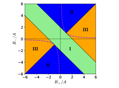
Figure 1: Regions of distinct spectrum for the operator (1) in the case of $B_{\pm}$ real (and $A>0$). I denotes the region with discrete positive spectrum (Eq. (32)), II that with continuous complex twofold degenerate spectrum (Eq. (46)) and III that with no convergent eigenfunctions (Eq. (60)). The dashed curves depict the set of points where ${\cal MH}$ is nondiagonalizable. The hermitian case corresponds to the line $B_{-}=B_{+}$.

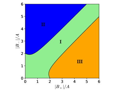
Figure 2: Regions of distinct spectrum for the operator (1) with complex $B_{\pm}=|B_{\pm}|e^{i\theta}$ and $\theta=\pi/6$. Same details as Fig. 1: In I, $H$ has a discrete complex spectrum, while in II it has a continuous complex spectrum and in III no convergent eigenfunctions. The dotted segment $|B_{+}|+|B_{-}|=2A$ indicates the upper limit of region I for $\theta=0$ ($B_{\pm}$ real and positive) whereas dotted lines $|B_{+}|-|B_{-}|=\pm 2A$ indicate the border of I for $\theta=\pi/2$ ($B_{\pm}$ imaginary); For general $\theta\in(0,\pi/2]$ and $|B_{\pm}|\gg A$, I is limited by lines $|B_{+}|-|B_{-}|=\pm 2A\sin\theta$.

On the other hand, when $\lambda$ is complex the spectrum of $H$ can be made real just by multiplying $H$ by a phase $\lambda^{*}/|\lambda|$, as seen from (29). The ensuing operator $H^{\prime}$ has the antiunitary symmetry $U{\cal T}$, with $U$ the Bogoliubov transformation $(^{a}_{a^{\dagger}})\rightarrow U(^{a}_{a^{\dagger}})U^{-1}=({\cal W}^{*})^{-1}{\cal W}(^{a}_{a^{\dagger}})$. For complex $\lambda$, the stable sector adopts the form depicted in Fig. 2 (sector I). For a common phase $\theta=0$ ($B_{\pm}$ real and positive) it is just the triangle $|B_{+}|+|B_{-}|<2A$, while for $\theta=\pi/2$ ($B_{\pm}$ imaginary, equivalent through a phase transformation to $B_{\pm}$ real with opposite signs) it corresponds to $||B_{+}|-|B_{-}||<2A$ (sectors delimited by dotted lines). The union of these two sectors leads to the stripe of Fig. 1 for $B_{\pm}$ arbitrary real numbers. For intermediate phases the stable region is essentially the union of the previous triangle with a narrower stripe, asymptotically delimited by the lines $||B_{+}|-|B_{-}||=2A\,\sin\theta$ for $|B_{\pm}|\gg A$. A similar type of diagram for a non-quadratic system was provided in Scholtz et al. (1992).

II.3 The coordinate representation

We now turn to the representation of $H$ and its eigenstates in terms of coordinate and momentum operators

$$Q=\frac{a+a^{\dagger}}{\sqrt{2}},\;\;P=\frac{a-a^{\dagger}}{i\sqrt{2}}\,,$$ (34)

satisfying $[Q,P]=i$. The Hamiltonian (2) becomes

$$H = \frac{1}{2}\left[\tilde{A}_{-}P^{2}+\tilde{A}_{+}Q^{2}+\tilde{B}\left(QP+PQ\right)\right]$$ (35)

$$= \begin{pmatrix}Q&P\end{pmatrix}\tilde{\cal H}\begin{pmatrix}Q\\ P\end{pmatrix},\;\tilde{\cal H}={\cal S}^{\dagger}{\cal H}{\cal S}=\begin{pmatrix}\tilde{A}_{+}&\tilde{B}\\ \tilde{B}&\tilde{A}_{-}\end{pmatrix},$$ (36)

where ${\cal S}=(^{1\;\;\;i}_{1\,-i})/\sqrt{2}$ and

$$\tilde{A}_{\pm}=A\pm\frac{B_{+}+B_{-}}{2},\quad\tilde{B}=\frac{B_{+}-B_{-}}{2i}\,.$$ (37)

The hermitian case corresponds to $\tilde{A}_{\pm}$ and $\tilde{B}$ real, while the generalized discrete positive spectrum case (33) to $\tilde{\cal H}+\tilde{\cal H}^{\dagger}>0$. Thus, for $B_{\pm}$ real the border $|B_{+}+B_{-}^{*}|=2A$ corresponds to $\tilde{A}_{-}=0$ or $\tilde{A}_{+}=0$, i.e. infinite mass or no quadratic potential, while for $B_{\pm}$ imaginary to $|\tilde{B}|=A$.

The diagonal form (3) can then be rewritten as

$$H=\frac{\lambda}{2}\left(P^{\prime\,2}+Q^{\prime\,2}\right),$$ (38)

where $Q^{\prime}=\frac{b+\bar{b}^{\dagger}}{\sqrt{2}}$ and $P^{\prime}=\frac{b-\bar{b}^{\dagger}}{i\sqrt{2}}$ satisfy $[Q^{\prime},P^{\prime}]=i$ but are in general no longer hermitian. They are related to $Q,P$ through a general canonical transformation

$$\begin{pmatrix}Q^{\prime}\\ P^{\prime}\end{pmatrix}=\tilde{\cal W}\begin{pmatrix}Q\\ P\end{pmatrix}\,,\;\;\;\tilde{\cal W}={\cal S}^{\dagger}{\cal W}{\cal S}=\begin{pmatrix}\frac{\alpha+\bar{\alpha}^{*}}{2}&-\frac{\beta-\bar{\beta}^{*}}{2i}\\ \frac{\alpha-\bar{\alpha}^{*}}{2i}&\frac{\beta+\bar{\beta}^{*}}{2}\end{pmatrix}\,,$$ (39)

where $(^{\alpha}_{\beta})=u\pm v$, $(^{\bar{\alpha}}_{\bar{\beta}})=\bar{u}\pm\bar{v}$ and ${\rm Det}(\tilde{\cal W})=1$. Here $\lambda$ can be expressed as

$$\lambda=\sqrt{\tilde{A}_{+}\tilde{A}_{-}-\tilde{B}^{2}}\,,$$ (40)

with $\pm\lambda$ the eigenvalues of $\tilde{\cal M}\tilde{\cal H}={\cal S}^{\dagger}{\cal M}{\cal H}{\cal S}$.

Setting $Q|x\rangle=x|x\rangle$, the coordinate representations $\psi_{0}^{b}(x)\equiv\langle x|0_{b}\rangle$, $\psi_{0}^{\bar{b}}(x)\equiv\langle x|0_{\bar{b}}\rangle$ of the vacua can be found from Eqs. (20) and (22). They can also be derived by solving the corresponding differential equations $\langle x|b|0_{b}\rangle=0$, $\langle x|\bar{b}|0_{\bar{b}}\rangle=0$, i.e.,

$$\left[\alpha x+\beta\partial_{x}\right]\psi_{0}^{b}(x)=0,\;\;\left[\bar{\alpha}x+\bar{\beta}\partial_{x}\right]\psi_{0}^{\bar{b}}(x)=0\,,$$ (41)

and read

$$\psi_{0}^{b}(x) \propto \exp\left[-\frac{\alpha}{2\beta}x^{2}\right],\;\;\psi_{0}^{\bar{b}}(x)\propto\exp\left[-\frac{\bar{\alpha}}{2\bar{\beta}}x^{2}\right]\,.$$ (42)

Since ${\rm Re}[\frac{z_{1}+z_{2}}{z_{1}-z_{2}}]=\frac{|z_{1}|^{2}-|z_{2}|^{2}}{|z_{1}-z_{2}|^{2}}$ $\forall$ $z_{1}\neq z_{2}\in\mathbb{C}$, it is verified that they have finite standard norms iff $|v|<|u|$ and $|\bar{v}|<|\bar{u}|$. The wave functions of the excited states $\Ket{n_{b}}$ and $\Ket{m_{\bar{b}}}$ can be similarly obtained by applying $\bar{b}^{\dagger}$ and $b^{\dagger}$ to the functions (42), according to Eq. (26):

$$\psi_{n}^{b}(x) = \frac{1}{\sqrt{n!}}\left[\sqrt{\frac{\bar{\beta}^{*}}{2\beta}}\right]^{n}H_{n}\left(\frac{x}{\gamma}\right)\psi_{0}^{b}(x),$$ (43)

$$\psi_{m}^{\bar{b}}(x) = \frac{1}{\sqrt{m!}}\left[\sqrt{\frac{\beta^{*}}{2\bar{\beta}}}\right]^{m}H_{m}\left(\frac{x}{\gamma^{*}}\right)\psi_{0}^{\bar{b}}(x),$$ (44)

where $\gamma=\sqrt{\beta\bar{\beta}^{*}}$ and $H_{n}(x)$ is the Hermite polynomial of degree $n$. These functions satisfy the biorthogonality relation (28), i.e., $\int_{-\infty}^{\infty}\psi_{m}^{\bar{b}*}(x)\psi_{n}^{b}(x)\mathrm{d}x=\delta_{mn}\Braket{0_{\bar{b}}}{0_{b}}$, with $\Braket{0_{\bar{b}}}{0_{b}}=1$ if normalization factors $(\sqrt{\pi}\beta)^{-1/2}$ and $(\sqrt{\pi}\bar{\beta})^{-1/2}$ are added in (42). They are verified to be the finite norm solutions to the Schrödinger equations associated with $H$ and $H^{\dagger}$ respectively. In the case of $\psi^{b}_{n}(x)$, the latter reads

$$-\frac{1}{2}\tilde{A}_{-}\psi^{\prime\prime}-i\tilde{B}\left[x\psi^{\prime}+\frac{\psi}{2}\right]+\frac{1}{2}\tilde{A}_{+}x^{2}\psi=E\psi\,,$$ (45)

with $E=\lambda(n+1/2)$, while in the case of $\psi_{m}^{\bar{b}}(x)$, $\tilde{A}_{\pm}$, $\tilde{B}$ are to be replaced by $\tilde{A}_{\pm}^{*}$ and $\tilde{B}^{*}$, with $E=\lambda^{*}(m+1/2)$.

II.4 The case of continuous spectrum

If $|v/u|<1$ but $|\bar{v}/\bar{u}|>1$, the vacuum $|0_{\bar{b}}\rangle$ of $\bar{b}$ is no longer well defined, since the coefficients of its expansion in the states $|n_{a}\rangle$, Eq. (22), become increasingly large for large $n$, and the associated eigenfunction $\psi_{0}^{\bar{b}}(x)$, Eq. (42), becomes divergent. This situation occurs whenever

$$\frac{|B_{+}|}{|B_{-}|}<\frac{|A-\lambda|}{|A+\lambda|}\,,$$ (46)

i.e.  below the window (24), and corresponds to regions II in Figs.  1 and 2. The same occurs with the excited states $\Ket{n_{\bar{b}}}$ defined in Eq.  (26).

Instead, it is now the operator $\bar{b}^{\dagger}$ which has a convergent vacuum, namely

$$\Ket{0_{\bar{b}^{\dagger}}}\propto\sum_{n=0}^{\infty}\left(-\frac{\bar{u}^{*}}{2\bar{v}^{*}}\right)^{n}\frac{\sqrt{2n!}}{n!}\Ket{2n_{a}},$$ (47)

satisfying $\bar{b}^{\dagger}\Ket{0_{\bar{b}^{\dagger}}}=0$. Since we can write $H$ as

$$H=-\lambda\,[(-b)\bar{b}^{\dagger}+1/2],$$ (48)

it becomes clear that $H\Ket{0_{\bar{b}^{\dagger}}}=-\lambda/2\,\Ket{0_{\bar{b}^{\dagger}}}$. Moreover, due to the commutation relation $[\bar{b}^{\dagger},-b]=1$, we may as well consider $-b$ as a creation operator and $\bar{b}^{\dagger}$ as an annihilation operator, and define the states

$$\Ket{n_{\bar{b}^{\dagger}}}=\frac{(-b)^{n}\Ket{0_{\bar{b}^{\dagger}}}}{\sqrt{n!}},$$ (49)

which then satisfy $-b\bar{b}^{\dagger}\Ket{n_{\bar{b}^{\dagger}}}=n\Ket{n_{\bar{b}^{\dagger}}}$, and hence

$$H\Ket{n_{\bar{b}^{\dagger}}}=-\lambda\left(n+\frac{1}{2}\right)\Ket{n_{\bar{b}^{\dagger}}}.$$ (50)

Since the previous states $|0_{b}\rangle$ and $\Ket{n_{b}}$ remain convergent, and Eq. (29) still holds, it is seen that $H$ posseses in this case two sets of discrete eigenstates constructed from the vacua of $b$ and $\bar{b}^{\dagger}$, with opposite energies. The wave functions of the “negative” band are given by

$$\psi_{0}^{\bar{b}^{\dagger}}(x) \propto\exp\left[\frac{\bar{\alpha}^{*}}{2\bar{\beta}^{*}}\,x^{2}\right],$$ (51)

$$\psi_{n}^{\bar{b}^{\dagger}}(x) \propto\frac{1}{\sqrt{n!}}\left[\sqrt{\frac{\beta}{2\bar{\beta}^{*}}}\right]^{n}H_{n}\left(\frac{ix}{\gamma}\right)\psi_{0}^{\bar{b}^{\dagger}}(x),$$

which are convergent since now $\mathrm{Re}(\bar{\alpha}^{*}/\bar{\beta}^{*})<0$.

However, these eigenvalues do not exhaust, remarkably, the entire spectrum. The Schrödinger equation (45) has in the present case two linearly independent bounded eigenstates $|\nu_{b}\rangle$ and $|\nu_{\bar{b}^{\dagger}}\rangle$, for any complex energy

$$E_{\nu}=\lambda\left(\nu+\frac{1}{2}\right),$$ (52)

with $\nu\in\mathbb{C}$. As demonstrated in the appendix, the associated eigenfunctions $\psi_{\nu}^{b}(x)=\Braket{x}{\nu_{b}}$ and $\psi_{\nu}^{\bar{b}^{\dagger}}(x)=\Braket{x}{\nu_{\bar{b}^{\dagger}}}$ are given explicitly by:

$$\psi_{\nu}^{b}(x) = \Xi(\nu)\left(\sqrt{\frac{\bar{\beta}^{*}}{2\beta}}\right)^{n}\exp\left(-\frac{i\tilde{B}+\lambda}{2\tilde{A}_{-}}\,x^{2}\right)\left[H_{\nu}\left(\frac{x}{\gamma}\right)+(-1)^{n}H_{\nu}\left(-\frac{x}{\gamma}\right)\right],$$ (53)

$$\psi_{\nu}^{\bar{b}^{\dagger}}(x) = \Xi(\nu)\left(\sqrt{\frac{\beta}{2\bar{\beta}^{*}}}\right)^{n}\exp\left(-\frac{i\tilde{B}-\lambda}{2\tilde{A}_{-}}\,x^{2}\right)\left[H_{\nu}\left(\frac{ix}{\gamma}\right)+(-1)^{n}H_{\nu}\left(-\frac{ix}{\gamma}\right)\right],$$ (54)

where $n=\lfloor\mathrm{Re}(\nu)\rfloor$, with $\lfloor x\rfloor$ the greatest integer lower than $x$ (floor function), and

$$\Xi(\nu)=\begin{cases}\sqrt{(|\nu|-1)!}&\quad\nu=-1,-2,\ldots\\ \frac{1}{\sqrt{\Gamma(\nu+1)}}&\quad\mbox{otherwise}\end{cases}\,.$$ (55)

For integer $\nu\geq 0$, these functions are proportional to the previous expressions (43) and (51). For general $\nu\in\mathbb{C}$, they satisfy

$$H\Ket{\nu_{b}} = \lambda\left(\nu+\frac{1}{2}\right)\Ket{\nu_{b}},$$ (56)

$$H\ket{\nu_{\bar{b}^{\dagger}}} = -\lambda\left(\nu+\frac{1}{2}\right)\Ket{\nu_{\bar{b}^{\dagger}}}\,,$$ (57)

with

$$b\Ket{\nu_{b}} \propto\sqrt{\nu}\Ket{\nu-1_{b}},$$ (58)

$$\bar{b}^{\dagger}\Ket{\nu_{b}} \propto\left\{\begin{array}[]{lcl}\sqrt{\nu+1}\Ket{\nu+1_{b}}&&(\nu\neq-1)\\ \Ket{0_{b}}&&(\nu=-1)\end{array}\right.\,,$$

$$\bar{b}^{\dagger}\Ket{\nu_{\bar{b}^{\dagger}}} \propto\sqrt{\nu}\Ket{\nu-1_{\bar{b}^{\dagger}}},$$ (59)

$$(-b)\Ket{\nu_{\bar{b}^{\dagger}}} \propto\left\{\begin{array}[]{lcl}\sqrt{\nu+1}\Ket{\nu+1_{\bar{b}^{\dagger}}}&&(\nu\neq-1)\\ \Ket{0_{\bar{b}^{\dagger}}}&&(\nu=-1)\end{array}\right.\,,$$

where the proportionality constant is a phase factor. Expressions (56)–(59) are in agreement with Eqs.  (17)–(18). They are valid in this region for both real or complex $\lambda$.

Note that if $\bar{b}^{\dagger}\Ket{\scalebox{0.6}[1.0]{$-$}1_{b}}$ would vanish, then $\Ket{\scalebox{0.6}[1.0]{$-$}1_{b}}$ would be proportional to $\Ket{0_{\bar{b}^{\dagger}}}$, which is not the case. A similar argument holds for $b\Ket{\scalebox{0.6}[1.0]{$-$}1_{\bar{b}^{\dagger}}}$. It is also verified that in the case of discrete spectrum (region I), such state $\Ket{\scalebox{0.6}[1.0]{$-$}1_{b}}$ does not exist, i.e., the solution of the first order differential equation $\Braket{x}{\bar{b}^{\dagger}}{\scalebox{0.6}[1.0]{$-$}1_{b}}=\Braket{x}{0_{b}}$ is divergent. In addition, we remark that Eqs. (53) and (54) are always linearly independent solutions of the Schrödinger equation (45), but in region I the function (54) is always divergent whereas (53) is divergent except for $\nu=n=0,1,2,\ldots$.

II.5 The case of no convergent eigenstates

If now $|\bar{v}/\bar{u}|<1$ but $|v/u|>1$, i.e.,

$$\frac{|B_{+}|}{|B_{-}|}>\frac{|A+\lambda|}{|A-\lambda|}\,,$$ (60)

neither $b$ nor $\bar{b}$ have a convergent vacuum, so that the eigenstates $\Ket{n_{b}}$ and $\Ket{n_{\bar{b}^{\dagger}}}$ of sec. II.2 are not well defined. In fact, Eqs. (53) and (54) become divergent for any $\nu$, so that $H$ has no convergent eigenfunctions for any value of $E$. This case corresponds to regions III in Figs. 1–2.

On the other hand, it is the operator $b^{\dagger}$ which now has a well defined vacuum $\Ket{0_{b^{\dagger}}}$, in addition to $\bar{b}$, which preserves its vacuum $|0_{\bar{b}}\rangle$. Therefore, one can define the states $\Ket{n_{b^{\dagger}}}$ and $\Ket{n_{\bar{b}}}$ in the same way as the treatment of previous section, and also $\Ket{\nu_{b^{\dagger}}}$ and $\Ket{\nu_{\bar{b}}}$ for any $\nu\in\mathbb{C}$, which will be eigenstates of $H^{\dagger}$. Hence, in this case $H^{\dagger}$, rather than $H$, has two linearly independent bounded eigenfunctions for every complex value of $E$. In contrast, in ${\bf II}$ $H^{\dagger}$ has no bounded eigenstate.

II.6 Non diagonalizable case

The matrix ${\cal MH}$ becomes non diagonalizable when $\lambda=0$, i.e. ${\rm rank}\,{\cal H}=1$. This case occurs whenever $B_{+}B_{-}=A^{2}$ and corresponds to the dashed curve in Fig. 1, which lies in regions II and III. The operator $H$ takes here the single square form (19).

We first analyze the sector lying in region II. In the limit $B_{+}\rightarrow 0$, with $B_{-}=A^{2}/B_{+}\rightarrow\infty$, $H$ becomes proportional to $a^{2}$. Its eigenstates then become the well known coherent states

$$|\alpha_{a}\rangle\propto\exp[\alpha a^{\dagger}]|0_{a}\rangle\,,$$ (61)

satisfying $a\Ket{\alpha_{a}}=\alpha\Ket{\alpha_{a}}$, $\alpha\in\mathbb{C}$, with $\frac{2B_{+}}{A^{2}}H\Ket{\pm\alpha_{a}}\rightarrow\alpha^{2}\Ket{\pm\alpha_{a}}$. This implies a continuous two-fold degenerate spectrum, as in the rest of region II. The spectrum of $H$ in II is then similar to that of $a^{2}$, reflecting the fact that here both $b$ and $\bar{b}^{\dagger}$ have a convergent vacuum and are then annihilation operators.

In fact, for $\lambda\rightarrow 0$ and $A>0$, the operators $b$ and $\bar{b}^{\dagger}$ of Eq. (4) become proportional, i.e. $\bar{b}^{\dagger}\rightarrow\sqrt{B_{-}/B_{+}}\,b$, such that $H\propto b^{2}$ at leading order. At the curve $\lambda=0$ and within region II, $H$ takes the exact form

$$H={\textstyle\frac{|B_{-}|-|B_{+}|}{2}\,\tilde{b}^{2},\;\;\;\;\tilde{b}=\frac{\sqrt{B_{-}}\,a+\sqrt{B_{+}}\,a^{\dagger}}{\sqrt{|B_{-}|-|B_{+}|}}},$$ (62)

where $\tilde{b}$ fulfills $[\tilde{b},\tilde{b}^{\dagger}]=1$ and has a convergent vacuum $\Ket{0_{\tilde{b}}}$ since here $|B_{+}|<|B_{-}|$. It then represents a proper annihilation operator. The eigenstates of $H$ become its coherent states $\Ket{\alpha_{\tilde{b}}}\propto\exp[\alpha\tilde{b}^{\dagger}]\Ket{0_{\tilde{b}}}$ satisfying $\tilde{b}\Ket{\alpha_{\tilde{b}}}=\alpha\Ket{\alpha_{\tilde{b}}}$, such that

$$H\Ket{\pm\,\alpha_{\tilde{b}}}={\textstyle\frac{|B_{-}|-|B_{+}|}{2}}\,\alpha^{2}\Ket{\pm\,\alpha_{\tilde{b}}}\,,$$ (63)

with $\alpha\in\mathbb{C}$. The spectrum is then complex continuous and two-fold degenerate, as in the rest of sector II. The eigenfunctions become

$$\psi_{\alpha}(x)=\Braket{x}{\alpha_{\tilde{b}}}\propto e^{-\frac{1}{2}\frac{\sqrt{B_{-}}+\sqrt{B_{+}}}{\sqrt{B_{-}}-\sqrt{B_{+}}}\left(x-\sqrt{2}\alpha\frac{\sqrt{|B_{-}|-|B_{+}|}}{\sqrt{B_{-}}+\sqrt{B_{+}}}\right)^{2}}.$$ (64)

On the other hand, in region III, $|B_{+}|>|B_{-}|$ and along the curve $\lambda=0$ we have instead

$$H={\textstyle\frac{|B_{+}|-|B_{-}|}{2}\,\tilde{b}^{\dagger\,2},\;\;\;\;\tilde{b}^{\dagger}=\frac{\sqrt{B_{-}}\,a+\sqrt{B_{+}}\,a^{\dagger}}{\sqrt{|B_{+}|-|B_{-}|}}},$$ (65)

with $\tilde{b}^{\dagger}$ a proper creation operator satisfying $[\tilde{b},\tilde{b}^{\dagger}]=1$ and having no bounded vacuum. Hence, here $H$ has no bounded eigenstates while $H^{\dagger}$ has has a continuous complex spectrum.

Finally, in the hermitian limit $|B_{+}|=|B_{-}|=A$, i.e. when the curve $\lambda=0$ crosses the border between II and III, $H\rightarrow\frac{A}{2}(e^{-i\phi}a+e^{i\phi}a^{\dagger})^{2}$, becoming proportional to $Q^{2}$ (or equivalently, to $P^{2}$ if $\phi=\pi/2$). It then possesses a continuous two-fold degenerate nonnegative real spectrum, although with non normalizable eigenstates ($\Ket{x}$ or $\Ket{p}$). This case corresponds in Fig. 1 to the two “critical” points where all three regions I, II, III merge, i.e., $|v/u|=|\bar{v}/\bar{u}|=1$. Thus, at the non-diagonalizable curve $\lambda=0$, $H$ is proportional to the square of: an annihilation operator inside region II, a creation operator inside region III, and a coordinate or momentum operator at the crossing with the Hermitian case.

II.7 Intermediate regions

We finally discuss the border between regions I and II or III. These intermediate lines have either $|v/u|=1$ or $|\bar{v}/\bar{u}|=1$. When crossing from I to II (III), $\bar{b}$ ($b$) undergoes an annihilation $\rightarrow$ creation transition, loosing its bounded vacuum and becoming at the crossing a coordinate or momentum.

As can be verified from Eqs. (53) and (54) when $\tilde{A}_{-}\neq 0$, at the border between I and II $H$ has still a discrete spectrum and satisfies Eq. (29), since (53) remains convergent just for $\nu=n$. On the other hand, (54) has no longer a finite norm since $(i\tilde{B}-\lambda)/(2\tilde{A}_{-})$ is an imaginary number. However, the dual states $\Ket{0_{\bar{b}}}$ and $\Ket{n_{\bar{b}}}$, while also lacking a finite norm $\Braket{n_{\bar{b}}}{n_{\bar{b}}}$, still have finite biorthogonal norms $\Braket{m_{\bar{b}}}{n_{b}}$, fulfilling Eq. (28). In contrast, at the border I-III $H$ ceases to have convergent eigenfunctions for any value of $\nu$, since $\Ket{n_{b}}$ stops being convergent, while dual states $\Ket{n_{\bar{b}}}$ remain convergent.

When $\tilde{A}_{-}=0$, which corresponds to the case $B_{\pm}$ real and $B_{+}+B_{-}=2A$ (the border between I and regions II–III in Fig. 1), we have $\bar{v}=\bar{u}$. In this case, and for $A\neq B_{-}$, Eq. (45) becomes of first order and has a unique solution given by

$$\psi_{\nu}^{b}(x)\propto e^{-\frac{Ax^{2}}{2(B_{-}-A)}}x^{\nu},$$ (66)

where we have set $E=\lambda(\nu+1/2)$, with $\lambda=B_{-}-A$, along this line. Hence, at the border with region III ($B_{-}<A$) Eq. (66) is always divergent for $|x|\rightarrow\infty$, while at the border with II it is always convergent for $|x|\rightarrow\infty$ yet regular at $x=0$ just for $\nu=n=0,1,2,\ldots$, as in the previous case. For these values, Eq. (66) becomes proportional to Eq. (43).

Regarding the dual states, at this line $\bar{b}=\bar{b}^{\dagger}=\sqrt{2}\bar{u}Q$, (since $\bar{u}$ is real) and as such $\Ket{0_{\bar{b}}}$ is the state with $Q=0$, i.e., $\Braket{x}{0_{\bar{b}}}\propto\delta(x)$. In fact, for $\bar{v}\rightarrow\bar{u}$ the coordinate representation of the state $\Ket{0_{\bar{b}}}$ in (22) becomes a delta function, as also seen from Eq. (42):

$$\Braket{x}{0_{\bar{b}}}\rightarrow\frac{e^{-x^{2}/2}}{\pi^{1/4}}\sum_{n=0}^{\infty}\frac{H_{2n}(x)H_{2n}(0)}{2^{2n}(2n)!}=\pi^{1/4}\delta(x),$$ (67)

where we have used $\delta(x)=\Braket{x}{0_{\bar{b}}}=\sum_{n=0}^{\infty}\langle x|n_{a}\rangle\langle n_{a}|0_{\bar{b}}\rangle$. It is then still verified that $\Braket{0_{\bar{b}}}{0_{b}}$ is a finite number. The same holds for the remaining states $\Ket{n_{\bar{b}}}$, with $\Braket{x}{n_{\bar{b}}}$ involving derivatives of the delta function, such that Eq. (28) still holds.

III The general $N$-dimensional case

We now discuss the main features of the $N$-dimensional case. We consider a general $N$-dimensional quadratic form in boson operators $a_{i}$, $a^{\dagger}_{j}$ satisfying $[a_{i},a^{\dagger}_{j}]=\delta_{ij}$, $[a_{i},a_{j}]=0$, $i,j=1,\ldots,N$:

$$H = \sum_{i,j}A_{ij}a^{\dagger}_{i}a_{j}+\frac{1}{2}(B^{+}_{ij}a^{\dagger}_{i}a^{\dagger}_{j}+B^{-}_{ij}a_{i}a_{j})$$ (68)

$$= \frac{1}{2}\begin{pmatrix}a^{\dagger}&a\end{pmatrix}{\cal H}\begin{pmatrix}a\\ a^{\dagger}\end{pmatrix}\,,\;\;{\cal H}=\begin{pmatrix}A&B_{+}\\ B_{-}&A^{T}\end{pmatrix}\,.$$ (69)

Here $B_{\pm}$ are symmetric $N\times N$ matrices of elements $B^{\pm}_{ij}$, such that ${\cal H}$ satisfies

$${\cal H}^{T}={\cal RHR}\,,\;\;{\cal R}=\begin{pmatrix}0&{\mathbbm{1}}\\ {\mathbbm{1}}&0\end{pmatrix}\,.$$ (70)

Following the treatment of Rossignoli and Kowalski (2005) for the general hermitian case, we define new operators $b_{i}$, $\bar{b}^{\dagger}_{i}$ through a generalized Bogoliubov transformation

$$\begin{pmatrix}b\\ \bar{b}^{\dagger}\end{pmatrix}={\cal W}\begin{pmatrix}a\\ a^{\dagger}\end{pmatrix},\;{\cal W}=\begin{pmatrix}U&V\\ \bar{V}^{*}&\bar{U}^{*}\end{pmatrix}\,,$$ (71)

where again $\bar{b}^{\dagger}_{i}$ may not coincide with $b^{\dagger}_{i}$ although the bosonic commutation relations are preserved:

$$[b_{i},\bar{b}^{\dagger}_{j}]=\delta_{ij},\;\;[b_{i},b_{j}]=[\tilde{b}_{i}^{\dagger},\tilde{b}_{j}^{\dagger}]=0.$$ (72)

These conditions imply Rossignoli and Kowalski (2005, 2009)

$${\cal WMRW}^{T}{\cal R}={\cal M}\,,$$ (73)

(${\cal M}$ is the matrix (10) extended to $2N\times 2N$) i.e.,

$$U(\bar{U}^{*})^{T}-V(\bar{V}^{*})^{T} = {\mathbbm{1}},$$ (74)

$$VU^{T}-UV^{T} = 0,\;\bar{V}\bar{U}^{T}-\bar{U}\bar{V}^{T}=0\,.$$ (75)

We can then rewrite $H$ exactly as in Eqs. (8)–(9):

$$H = \frac{1}{2}\begin{pmatrix}\bar{b}^{\dagger}&b\end{pmatrix}\mathcal{H}^{\prime}\begin{pmatrix}b\\ \bar{b}^{\dagger}\end{pmatrix}\,,\;\mathcal{H}^{\prime}={\cal M}{\cal W}{\cal M}{\cal H}{\cal W}^{-1}\,,$$ (76)

where ${\cal H}^{\prime}$ has again the form (69) and satisfies (70) due to Eq. (73). The problem of obtaining a normal mode representation

$$H=\sum_{i}\lambda_{i}(\bar{b}_{i}^{\dagger}b_{i}+\frac{1}{2})\,,$$ (77)

leads then to the diagonalization of the matrix

$${\cal MH}=\begin{pmatrix}A&B_{+}\\ -B_{-}&-A^{T}\end{pmatrix},$$ (78)

which is that representing the commutation relations of Eq. (14) in the present general case: $[H,(^{a}_{a^{\dagger}})]={\cal MH}(^{a}_{a^{\dagger}})$.

A basic result is that the eigenvalues of (78) always come in pairs of opposite sign, as in the hermitian case Rossignoli and Kowalski (2005) (see also Fernández (2016)): Noting that ${\cal RM}=-{\cal MR}$ and ${\cal M}^{2}={\cal R}^{2}={\mathbbm{1}}$, Eq. (70) implies

$$({\cal MH}-\lambda{\mathbbm{1}})^{T}={\cal RHRM}-\lambda{\mathbbm{1}}={\cal RM}({\cal MH}+\lambda{\mathbbm{1}}){\cal RM}$$

and hence ${\rm Det}[{\cal MH}-\lambda{\mathbbm{1}}]={\rm Det}[{\cal MH}+\lambda{\mathbbm{1}}]$, entailing that if $\lambda$ is an eigenvalue of ${\cal M}{\cal H}$, so is $-\lambda$.

From Eq. (70) we also see that if $Z_{i}$ are eigenvectors of ${\cal MH}$ satisfying ${\cal M}{\cal H}Z_{i}=\lambda_{i}Z_{i}$, then $Z_{i}^{T}{\cal RM}Z_{j}(\lambda_{i}+\lambda_{j})=0$, implying the orthogonality relations

$$Z_{i}^{T}{\cal RM}Z_{j}=0\;\;\;\;(\lambda_{i}\neq-\lambda_{j})\,.$$ (79)

The pairs $(b_{i},\bar{b}^{\dagger}_{i})$ emerge then from the eigenvectors $Z_{i},Z_{\bar{i}}$ associated to opposite eigenvalues $\pm\lambda_{i}$, which are to be scaled such that

$$Z_{i}^{T}{\cal RM}Z_{\bar{i}}=1\,.$$ (80)

Writing $Z_{i}=\begin{pmatrix}\bar{U}^{*}&-\bar{V}^{*}\end{pmatrix}^{T}_{i}$ and $Z_{\bar{i}}=\begin{pmatrix}-V&U\end{pmatrix}^{T}_{i}$, we can form with them the eigenvector matrix ${\cal W}^{-1}$, with Eqs. (79)–(80) ensuring that ${\cal W}$ will satisfy Eq. (73).

Therefore, if ${\cal MH}$ is diagonalizable, a diagonalizing matrix ${\cal W}$ satisfying (73) will exist such that $H$ can be written in the diagonal form (77). The $N$-dimensional $H$ can then be reduced to a sum of $N$ commuting one-dimensional systems (complex normal modes) described by operators $H_{i}=\lambda_{i}(\bar{b}^{\dagger}_{i}b_{i}+\frac{1}{2})$. The normal operators $b_{i}$, $\bar{b}^{\dagger}_{i}$, satisfy

$$[H,b_{i}]=-\lambda_{i}b_{i},\;\;[H,\bar{b}^{\dagger}_{i}]=\lambda_{i}\bar{b}^{\dagger}_{i}\,,$$ (81)

diagonalizing the commutator algebra with $H$ and satisfying then Eqs. (17)–(18) $\forall$ $b=b_{i}$.

Now, if a common vacuum $|0_{b}\rangle$ exists such that

$$b_{i}|0_{b}\rangle=0\,,$$ (82)

for $i=1,\ldots,N$, it must necessarily be of the form Ring and Schuck (1980)

$$|0_{b}\rangle\propto\exp[-\frac{1}{2}\sum_{i,j}(U^{-1}V)_{ij}a^{\dagger}_{i}a^{\dagger}_{j}]|0_{a}\rangle\,,$$ (83)

where $U^{-1}V$ is a symmetric matrix due to Eq. (75). Eq. (83) can be directly checked by application of $b_{i}$. Similarly, assuming a common vacuum $|0_{\bar{b}}\rangle$ exists such that

$$\bar{b}_{i}|0_{\bar{b}}\rangle=0\,,$$ (84)

for $i=1,\ldots,N$, it must be of the form

$$|0_{\bar{b}}\rangle\propto\exp[-\frac{1}{2}\sum_{i,j}(\bar{U}^{-1}\bar{V})_{ij}a^{\dagger}_{i}a^{\dagger}_{j}]|0_{a}\rangle\,.$$ (85)

Assuming these series are convergent, which implies that $U^{-1}V$ and $\bar{U}^{-1}\bar{V}$ have both all singular values $\sigma_{i}<1$, $\bar{\sigma}_{i}<1$, we can define the states

$$|n_{1},\ldots,n_{N}\,{}_{b}\rangle = \left(\prod_{i}\frac{(\bar{b}^{\dagger}_{i})^{n_{i}}}{\sqrt{n_{i}!}}\right)|0_{b}\rangle,$$ (86)

$$|m_{1},\ldots,m_{N}\,{}_{\bar{b}}\rangle = \left(\prod_{i}\frac{(b^{\dagger}_{i})^{m_{i}}}{\sqrt{m_{i}!}}\right)|0_{\bar{b}}\rangle\,.$$ (87)

Due to the commutation relations (72), these states form again a biorthogonal set,

$$\langle m_{1},\ldots,m_{N}\,{}_{\bar{b}}|n_{1},\ldots,n_{N}\,{}_{b}\rangle=\delta_{m_{1}n_{1}}\ldots\delta_{m_{N}n_{N}}\langle 0_{\bar{b}}|0_{b}\rangle\,,$$ (88)

and satisfy

$$H||n_{1},\ldots,n_{N}\,{}_{b}\rangle = \sum_{i}\lambda_{i}\left(n_{i}+\frac{1}{2}\right)|n_{1},\ldots,n_{N}\,{}_{b}\rangle,$$ (89)

$$H^{\dagger}|m_{1},\ldots,m_{N}\,{}_{\bar{b}}\rangle = \sum_{i}\lambda_{i}^{*}\left(m_{i}+\frac{1}{2}\right)|m_{1},\ldots,m_{N}\,{}_{\bar{b}}\rangle\,.$$ (90)

Thus, both $H$ and $H^{\dagger}$ possess in this case a discrete spectrum. Such spectrum can be real if $H$ has some antilinear (generalized ${\cal PT}$) symmetry (for instance, ${\cal H}$ real).

In a general situation, a common vacuum may exist just for a certain subset of operators $b_{i}$ and $\bar{b}_{i}$, leading to terms $H_{i}$ with behaviors similar to those encountered in the previous section. An important difference is to be found in the non-diagonalizable cases: The corresponding modes may not necessarily be of the form (19), and are not necessarily associated with vanishing eigenvalues $\lambda_{i}=0$, since Jordan forms of higher dimension can arise, as was already shown in two-dimensional systems Rossignoli and Kowalski (2009); Rebón et al. (2014), in the context of hermitian yet unstable Hamiltonians. Besides, ${\cal MH}$ may remain diagonalizable in the presence of vanishing eigenvalues Rossignoli and Kowalski (2009); Colpa (1986).

IV Conclusions

We have first analyzed the spectrum and normal modes of a general one-dimensional quadratic bosonic form, showing that it can exhibit three distinct regimes:
i) An harmonic phase characterized by a discrete spectrum of both $H$ and $H^{\dagger}$, with bounded eigenstates constructed from gaussian vacua, which form a biorthogonal set. Such phase, which comprises the cases considered in Swanson (2004); Jones (2005), arises when the deviation from the stable hermitian case is not “too large” (Eq. (24), equivalent to (32)–(33) for $\lambda>0$), in which case the generalized normal boson operators $\bar{b}^{\dagger}$, $b$ can be considered as creation and annihilation operators respectively. According to the phase of $\lambda$, the discrete spectrum can be real or complex, but in the latter it can be made real by applying a trivial phase factor (as opposed to discrete regimes in nonquadratic Hamiltonians Fernández and Garcia (2014b)).

ii) A coherent-like phase where $H$ exhibits a complex twofold degenerate continuous spectrum while $H^{\dagger}$ has no bounded eigenstates. It corresponds to large deviations from the hermitian harmonic case. The normal operators $\bar{b}^{\dagger}$, $b$ can be considered as a pair of annihilation operators, each with a convergent vacuum yet still satisfying a bosonic commutator. The spectrum is then similar to that of a square of a bosonic annihilation operator.

iii) An adjoint coherent phase where $H^{\dagger}$ has a continuous complex spectrum while $H$ has no bounded eigenstates. Here the normal modes are a pair of creation operators. While ii) and iii) might be considered as having no proper biorthogonal eigenstates, the convergent eigenstates (of $H$ or $H^{\dagger}$) constitute a generalization of the standard coherent states, which arise here in the particular case of a non-diagonalizable matrix ${\cal MH}$. These regimes may be considered to correspond to a broken generalized ${\cal PT}$ symmetry, since there are complex eigenvalues. Nonetheless, the latter do not emerge from the coalescence of two or more real eigenvalues Bender (2007) but from the onset of convergence of eigenstates with complex quantum number $\nu$.

We have also analyzed the transition curves between these previous regimes, where one of the operators changes from creation to annihilation (or viceversa). At these curves such operator is actually a coordinate (or momentum), and even though there is just a discrete spectrum (with bounded eigenstates) of either $H$ or $H^{\dagger}$, the biorthogonality relations are still preserved. Explicit expressions for eigenfunctions were provided in all regimes.

The normal mode decomposition of the $N$-dimensional non-hermitian case has also been discussed, together with the corresponding harmonic regime. It opens the way to investigate in detail along these lines the spectrum of more complex specific non-hermitian quadratic systems.

*

Appendix A Solutions of the Schrödinger equation in the case of continuous spectrum

The solutions to the Schrödinger equation (45) can be obtained by making the substitution

$$\psi(x)=\exp\left[-\frac{i\tilde{B}+\lambda}{2\tilde{A}_{-}}x^{2}\right]\phi\left(\frac{x}{\gamma}\right).$$ (91)

We obtain the Hermite equation Lebedev (1965):

$$\phi^{\prime\prime}(z)-2z\phi^{\prime}(z)+2\nu\phi(z)=0,$$ (92)

with $z=x/\gamma$ and $\nu=(2E-\lambda)/(2\lambda)$. For complex $\nu$, four solutions are:

$$\phi_{\nu}^{(1)}(z)=H_{\nu}(z), \quad\phi_{\nu}^{(2)}(z)=H_{\nu}(-z)$$ (93)

$$\phi_{\nu}^{(3)}(z)=e^{z^{2}}H_{-\nu-1}(iz), \quad\phi_{\nu}^{(4)}(z)=e^{z^{2}}H_{-\nu-1}(-iz),$$

where $H_{\nu}$ are the Hermite functions Lebedev (1965). Since the Hermite equation is of second order, any of these solutions can be written as a linear combination of two others. For instance, for real $A,B_{+},B_{-}>0$:

$$H_{\nu}(z) =\frac{2^{\nu}\Gamma(\nu+1)}{\sqrt{\pi}}e^{z^{2}}\left[e^{\nu\pi i/2}H_{-\nu-1}(iz)\right.$$ (94)

$$\left.+e^{-\nu\pi i/2}H_{-\nu-1}(-iz)\right].$$

Additionaly, note that for integer $\nu\geq 0$, $\phi_{1}=(-1)^{\nu}\phi_{2}$ whereas for integer $\nu<0$, $\phi_{3}=(-1)^{\nu+1}\phi_{4}$.

The asymptotic behaviour of the Hermite functions for $|\arg z|<3/4$ goes as follows:

$$H_{\nu}(z)\sim(2z)^{\nu}+O(|z|^{\nu-2}),$$ (95)

and for $\pi/4+\delta\leq\arg z\leq 5\pi/4-\delta$ (which includes $z$ on the real negative axis):

$$H_{\nu}(z) \sim(2z)^{\nu}\left[1+O(|z|^{-2})\right]-$$ (96)

$$\frac{\sqrt{\pi}e^{\nu\pi i}}{\Gamma(-\nu)}e^{z^{2}}z^{-\nu-1}\left[1+O(|z|^{-2})\right].$$

Note that:

$$e^{z^{2}}\exp\left[-\frac{i\tilde{B}+\lambda}{2\tilde{A}_{-}}x^{2}\right]=\exp\left[-\frac{i\tilde{B}-\lambda}{2\tilde{A}_{-}}x^{2}\right].$$ (97)

For hermitian $H$, $\tilde{B}$ is either a real number or zero, and $\lambda$ determines whether the eigenfunctions are bounded or not (i.e., if $\lambda$ is real and positive then there are some bounded eigenfunctions, whereas for $\lambda$ negative or imaginary every eigenfunction is divergent). In such case, for positive, integer $\nu$ only $\phi_{\nu}^{(1)}$ (and $\phi_{\nu}^{(2)}$, since they are linearly dependent) may be bounded (see Eq. (96)), and for other values of $\nu$ there are no bounded eigenfunctions. On the other hand, for non-Hermitian $H$, the convergence of both linearly independent eigenstates may be assured provided that $\mathrm{Re}[(i\tilde{B}-\lambda)/\tilde{A}_{-}]>0$, which is fulfilled in region II, i.e., when both $b$ and $\bar{b}^{\dagger}$ have convergent vacua. Moreover, both linearly independent eigenstates may be convergent even if $\lambda$ is an imaginary number or zero, which implies for real $A,B_{\pm}$, that region II extends into the imaginary part of the spectrum in Fig. 1.

The eigenfunctions of $H$ must then be constructed from (93) in such a way that they behave as the eigenstates $\Ket{n_{b}}$ and $\Ket{n_{\bar{b}^{\dagger}}}$, i.e., they satisfy Eqs. (26) and (27), and they must be even or odd with respect to coordinate inversion $x\rightarrow-x$ (since the Hamiltonian is parity invariant). These considerations lead to the eigenfunctions (53) and (54).