Boxy Orbital Structures in Rotating Bar Models

Abstract

We investigate regular and chaotic two-dimensional (2D) and three-dimensional (3D) orbits of stars in models of a galactic potential consisting in a disk, a halo and a bar, to find the origin of boxy components, which are part of the bar or (almost) the bar itself. Our models originate in snapshots of an $N$-body simulation, which develops a strong bar. We consider three snapshots of the simulation and for the orbital study we treat each snapshot independently, as an autonomous Hamiltonian system. The calculated corotation-to-bar-length ratios indicate that in all three cases the bar rotates slowly, while the orientation of the orbits of the main family of periodic orbits changes along its characteristic. We characterize the orbits as regular, sticky, or chaotic after integrating them for a 10 Gyr period by using the GALI₂ index. Boxiness in the equatorial plane is associated either with quasi-periodic orbits in the outer parts of stability islands, or with sticky orbits around them, which can be found in a large range of energies. We indicate the location of such orbits in diagrams, which include the characteristic of the main family. They are always found about the transition region from order to chaos. By perturbing such orbits in the vertical direction we find a class of 3D non-periodic orbits, which have boxy projections both in their face-on and side-on views.

1 INTRODUCTION

Strong bars are observed in optical images of almost half of all nearby disk galaxies (see e.g. Barazza et al., 2008; Marinova & Jogee, 2007; Reese et al., 2007). This percentage increases nearly to $70$ % when near-infrared images are considered (Knapen et al., 2000; Menéndez-Delmestre et al., 2007; Eskridge et al., 2000). Bars are characterized by three parameters: length, strength, and pattern speed. This last parameter is defined as the rotational frequency of the bar and determines to a large extent the dynamics of a barred galaxy. Bars are classified as fast or slow by means of the ratio $R=R_{CR}/a_{b}$, where $R_{CR}$ is the corotation radius, and $a_{b}$ is the length of the semi-major axis of the bar. The orbital theory shows that bars cannot extend beyond corotation (Contopoulos, 1980). In the case of fast rotators we have $1.0<R<1.4$, while for slow rotators $R>1.4$ (Athanassoula, 1992b; Debattista & Sellwood, 2000). By definition, in a slow rotator, corotation is located far from the end of the bar.

Structures in barred galaxies have to be supported by stellar orbits (Contopoulos, 2002; Binney & Tremaine, 2008). It is now known that not only regular, but chaotic, sticky orbits as well can be used for building the bars (Wozniak, 1994; Kaufmann & Contopoulos, 1996; Patsis et al., 1997; Wozniak & Pfenniger, 1999; Muzzio et al., 2005; Harsoula & Kalapotharakos, 2009; Harsoula et al., 2010; Patsis et al., 2010; Contopoulos & Harsoula, 2013; Patsis & Katsanikas, 2014b; Tsigaridi & Patsis, 2015). Sticky orbits are chaotic orbits which wander for relatively long times close to the outer borders of stability islands before eventually entering a well defined chaotic region in the system’s phase space. In some other cases there is also stickiness near unstable asymptotic curves in the chaotic sea, which is called “stickiness in chaos” (Contopoulos & Harsoula, 2008). In both cases, sticky orbits mimic the behaviour of quasi-periodic orbits in the configuration space during the time they remain confined in a region of phase space. However, ultimately, during their time evolution they will exhibit a change in their orbital morphology as they will at a certain time change their behavior from quasi-regular to completely chaotic.

Special features and deviations from the standard orbital dynamics (Contopoulos & Grosbol, 1989) have been encountered in several cases. For example, in Tsigaridi & Patsis (2015) the orbital stellar dynamics of a two-dimensional (2D), slowly rotating, barred-spiral model has been investigated. In this case, orbital families have been presented that support in the galactic plane an inner ring and an X feature embedded in the bar. However, the dynamics associated with this model is different from that of a typical bar ending close to corotation. The ring was a result of a folding of the characteristic (“S” shape), along which the orientation of the elliptical orbits of the main family, as well as their stability vary (bistable bifurcation). On the other hand the observed boxiness and the X feature reflected the presence of sticky orbits at energy levels corresponding to the middle of the barred-spiral potential. Folding of the characteristic curve of the main planar family has been found earlier in the work of Skokos et al. (2002b) in the case of a 3D bar rotating again slowly. A question that arises is how common this feature is in the backbone families of real bars and what are the implications for the observed morphologies.

The aim of this work is to study the underlying dynamics in three analytic models that have a common origin, being derived from snapshots of an $N$-body simulation reported in Machado & Athanassoula (2010). We want to examine the degree of chaoticity of the bar-supporting orbits. In that simulation the interaction between the dark matter halo and the disk develops a bar, which evolves in time. We consider for our study three snapshots at times 4.2, 7 and 11.2 Gyr. Each snapshot is modeled by a frozen potential and so we treat each one of them as a time independent model, i.e. we use in our work the formalism for autonomous Hamiltonian systems. The bar is modeled with a Ferrers potential (Ferrers, 1877), the disk is a Miyamoto-Nagai disk (Miyamoto & Nagai, 1975) and the dark matter halo is these snapshots have been taken from Manos & Machado (2014) (hereafter MM). Throughout the text, by referring to a “snapshot” we will refer to the corresponding model in MM.

In particular we want to examine the relation between morphological features of the bars and the degree of chaos of the orbits that support these features. Such features include a possible inner and/or outer boxiness of the bar and the formation of rings. In the 3D barred models in Patsis & Katsanikas (2014a, b) it has been suggested that inner boxy features can be built by means of quasi-periodic orbits at the edges of the stability islands of the x1 family, as well as with sticky orbits just beyond the last invariant torus around the stable x1 periodic orbit. It has been also proposed that such orbits support boxiness both in face-on, as well as in edge-on projections at the central region of the bar (about within half the way to the end of the bar). A similar dynamical phenomenon was leading to the boxy features on the galactic plane in the bars of 2D barred-spiral models in Tsigaridi & Patsis (2015).

In the present study we want to investigate what kind of orbits support double boxy morphologies in the successive snapshots, and how they evolve in time, i.e. from the model of the earlier snapshot to the model for the final one. We want to examine whether this dynamical mechanism is associated with orbits just beyond the vertical 2:1 resonance region, or can be applied in a large energy range in which we can find bar-supporting orbits. For this purpose we do not investigate in detail the structure of phase space in a large number of energies, but we investigate the systems’ global dynamics using chaos indicators.

Many techniques have been developed over the years for determining the regular or chaotic nature of orbits of dynamical systems. Review presentations of some of the most commonly used methods can be found in Skokos et al. (2016). Among these chaos indicators the Smaller Alignment Index (SALI) method (Skokos, 2001; Skokos et al., 2003, 2004) and its extension, the Generalized Alignment Index (GALI) technique (Skokos et al., 2007, 2008; Manos et al., 2012) proved to be quite efficient in revealing the chaotic nature of orbits of Hamiltonian systems in a fast and accurate way. The computation of these indices is based on the time evolution of more than one deviations from the studied orbits. The SALI/GALI methods have already been successfully applied to dynamical studies of astronomical problems (see e.g. Sándor et al., 2004; Capuzzo-Dolcetta et al., 2007; Soulis et al., 2007; Voglis et al., 2007; Manos et al., 2008; Voyatzis, 2008; Bountis & Papadakis, 2009; Harsoula & Kalapotharakos, 2009; Manos & Athanassoula, 2011; Manos et al., 2013; Carpintero et al., 2014; Machado & Manos, 2016). The reader is referred to Skokos & Manos (2016) for a recent review of the theory and applications of the SALI/GALI chaos indicators.

In order to study the degree of chaoticity of the orbits of our models we use the GALI₂ index, whose time evolution reveals quite efficiently the regular, sticky or chaotic nature of the studied orbit. It can also tell the time interval within which a sticky orbit behaves as a regular one, being able this way to support a given morphological structure. For these reasons the use of GALI₂ is an essential tool for the needs of our investigation. We also note here that the GALI₂ index is closely related to the SALI method (see for example Appendix B of Skokos et al., 2007).

The paper is organized as follows: In section 2 we explain the gravitational potentials that model the components of the $N$-body snapshots. In section 3 we present the numerical methods used in our study. In particular we introduce the Hamiltonian of the system. The GALI₂ index is introduced as well. In section 4 we present the results of our study. We describe the characteristic curves of the main planar family of periodic orbits in the models we study and we label the initial conditions of the integrated non-periodic orbits, according to the degree of their chaoticity. Finally in section 5 we summarize our findings and we present and discuss our conclusions.

2 Modelling the $N$-body snapshots

In our study we follow closely the approach of the work of MM. The models used for approximating the morphologies encountered in the studied snapshots of the $N$-body simulation consist of a bar embedded in an axisymmetric disk and halo environment. The bar is represented by a Ferrers model (Ferrers 1877), the disk is a typical Miyamoto-Nagai model (Miyamoto & Nagai, 1975) and the spherical dark mater halo surrounding the disk is represented by a Dehnen potential (Dehnen, 1993). The mathematical formulae for these potentials can be found in MM.

The structural and dynamical parameters of the bar, disk and halo of the models are adopted from the models in MM and are summarized in Table 1. In this table we include also an earlier snapshot presented in MM, at $t=1.4$ Gyr, which however has not developed yet a strong bar. We keep it in the table, but we will not present any orbital analysis for its small bar. Thus, the models in Table 1 correspond to four snapshots taken at times $t=1.4$ Gyr, $t=4.2$ Gyr, $t=7.0$ Gyr, and $t=11.2$ Gyr. We name them snapshot “1”, “2”, “3” and “4” respectively.

The scaling of units we used in our calculations, which corresponds also to the numbers that appear in the axes of the figures in this work, are: 1 kpc (length), $2\times 10^{11}M_{\odot}$ (mass), 1 kpc²/Myr² (energy), while G = 1.

Table 1: The parameters of the models fitting the snapshots of the $N$-body simulation of Manos & Machado (2014). Successively we give the number of the snapshot (s/s), the time of the snapshot, the semi-axes of the Ferrers bar $(a,b,c)$, the pattern speed of the bar $\Omega_{b}$, the mass of the bar $M_{B}$, the scale lengths of the Miyamoto disk $A$ and $B$, the disk mass $M_{D}$, the scale radius of the halo $a_{H}$, the dimensionless parameter $\gamma$ in the Dehnen halo potential and the mass of the halo $M_{H}$ (units as in the MM paper).

				Bar					Disk				Halo
s/s	time		$a$	$b$	$c$	$\Omega_{b}$	$M_{B}$		$A$	$B$	$M_{D}$		$a_{H}$	$\gamma$	$M_{H}$
	(Gyr)		(kpc)	(kpc)	(kpc)	(km s-1 kpc-1)	($10^{10}M_{\odot}$)		(kpc)	(kpc)	($10^{10}M_{\odot}$)		(kpc)		($10^{10}M_{\odot}$)
1	1.4		2.24	0.71	0.44	52	1.04		1.92	0.22	3.96		3.90	0.23	25
2	4.2		5.40	1.76	1.13	24	2.36		0.95	0.53	2.64		5.21	0.71	25
3	7.0		7.15	2.38	1.58	14	3.02		0.78	0.56	1.98		5.77	0.85	25
4	11.2		7.98	2.76	1.93	9	3.30		0.71	0.59	1.70		5.95	0.89	25

Having available the parameters of each model we consider as length of the bar the length of the semi-major axis of the Ferrers bar, $a$. Also, from the pattern speed of each model, $\Omega_{b}$, we compute the location of the Lagrangian points $L_{1}$ and $L_{2}$. We consider as corotation radius their distance from the center of the system. Then we calculated the ratio $R=R_{CR}/a_{b}=R_{L_{1}}/a$. For the three models we analyzed, the values we found are given in Table 2.

Table 2: Parameters associated with the pattern speed of the studied models. Each row gives successively name of the snapshot, the time after the beginning of the simulation it is taken, the radius of the Lagrangian point $L_{1}$ and the corotation-to-bar’s length ratio.

snapshot 2	$t=4.25$ Gyr	$R_{L_{1}}=10.83$	$R=2.0$
snapshot 3	$t=7.00$ Gyr	$R_{L_{1}}=16.46$	$R=2.3$
snapshot 4	$t=11.2$ Gyr	$R_{L_{1}}=22.88$	$R=2.87$

We note that the $R_{L_{4}}$ values are very close o the $R_{L_{1}}$ ones, being 10.75, 16.37 and 22.89 respectively. We realize that in all cases $R>1.4$, which places all models to the class of slow rotators.

3 Autonomous Hamiltonian system and the GALI₂ index

The Hamiltonian of the system is given by

$$H=\frac{1}{2}(p_{x}^{2}+p_{y}^{2}+p_{z}^{2})+\Phi(x,y,z)-\Omega_{b}(xp_{y}-yp_{x})=E_{J}$$ (1)

where $x,y,z$ are Cartesian coordinates, $p_{x},p_{y},p_{z}$ are the conjugate momenta in the inertial reference frame, and $\Omega_{b}$ is the pattern speed of the bar. $E_{J}$ is the energy of Jacobi and $\Phi=\Phi_{B}+\Phi_{D}+\Phi_{H}$. where $\Phi_{B}$ is the potential of the bar, $\Phi_{D}$ is the potential of the disk, and $\Phi_{H}$ is the potential of the halo.

The equations of motion and the variational equations we use in order to follow the evolution of the two deviation vectors from the studied orbit can be found in the MM paper. They are needed for computing the GALI₂ index.

The GALI₂ index is given by the absolute value of the wedge product of two normalized to unity deviation vectors $\mathbf{\hat{w}}_{1}(t)$ and $\mathbf{\hat{w}}_{2}(t)$:

$$\rm{GALI}_{2}(t)=|\mathbf{\hat{w}}_{1}(t)\wedge\mathbf{\hat{w}}_{2}(t)|.$$ (2)

(see MM for details).

Thus, in order to evaluate GALI₂ we integrate the equations of motion and the variational equations for two deviation vectors simultaneously. The GALI₂ index behaves as follows (see Skokos & Manos, 2016, and references therein):

• For chaotic orbits it falls exponentially to zero as:

  $$\mbox{GALI}_{2}(t)\propto\exp{(-(\lambda_{1}-\lambda_{2})t)}$$ (3)

  where $\lambda_{1}$ and $\lambda_{2}$ are the two largest Lyapunov exponents (for the computation of the Lyapunov exponents see: Benettin et al., 1980; Skokos, 2010).

• For regular orbits it oscillates around a positive value across the integration:

  $$\mbox{GALI}_{2}(t)\propto constant.$$ (4)

• In the case of sticky orbits we observe a transition from practically constant GALI₂ values, which correspond to the seemingly quasi-periodic epoch of the orbit, to an exponential decay to zero, which indicates the orbit’s transition to chaoticity.

4 The degree of chaoticity of the orbits

4.1 Planar orbits

In a rotating Ferrers bar the elliptical periodic orbits of the main families are characterized by a single non-zero initial condition along the minor axis of the bar, namely their position along the y-axis in our models. The curve of zero velocity (ZVC) in a $(E_{J},y_{0})$ diagram separates the region where orbital motion is allowed from the region where it is not. Since the main family consists of direct periodic orbits, only the $y_{0}>0$ part of such a diagram is of interest for us. An $(E_{J},y_{0})$ diagram is the projection of a complete $(E_{J},y_{0},p_{y_{0}})$ figure with all possible initial conditions. However, it is sufficient for describing the properties of the orbits we present below. The line that gives the $y_{0}$ initial condition of the main family of periodic orbits is the characteristic curve of the model. Since we want to study chaoticity in a large range of energies, we have created such $(E_{J},y_{0})$ diagrams for the potentials of the three snapshots we study. In order to calculate the degree of chaoticity of the planar orbits around the main family of periodic orbit as we move from the center of the system towards corotation, we use the GALI₂ index. We have used the GALI₂ index to color-code each point in the allowed region in the $(E_{J},y_{0})$ areas. The shade of the color indicates the GALI₂ index that a given orbit, i.e. a point in the $(E_{J},y_{0})$ diagram, has at the end of the integration. In other words, the color of an $(E_{J},y_{0})$ point indicates if the orbit with $y_{0}$ initial condition at $E_{J}$ will lead to regular (large $\log_{10}(\mbox{GALI}_{2})$ values) or chaotic (very small $\log_{10}(\mbox{GALI}_{2})$ values) motion. At the borders between these regions we find points with intermediate $\log_{10}(\mbox{GALI}_{2})$ values, which correspond to sticky chaotic orbits.

4.1.1 Snapshot 2, t=4.2 Gyr

For each model we sample the GALI₂ index at two time windows. First after time $t_{1}$, corresponding to 1 Gyr and then after time $t_{2}$, corresponding to 10 Gyr. In this way we investigate both the relatively short-term as well as the long-term behaviour of the orbits. The two color-coded $(E_{J},y_{0})$ diagrams for snapshot “2” are given in Fig. 1. Fig. 1a gives the index after $t_{1}=$ 1 Gyr and Fig. 1b after $t_{2}=$ 10 Gyr.

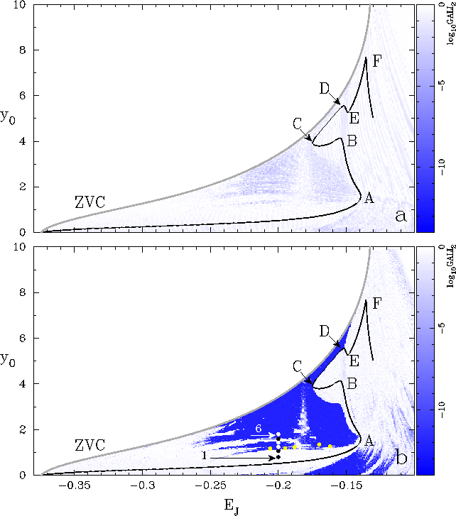
Figure 1: The chaoticity of the planar orbits on the equatorial plane of model “2” is given color coded in $(E_{J},y_{0})$ diagrams. The colour of each orbit (each point in the figures) corresponds to the value of the $\log_{10}$(GALI₂) quantity calculated for it and is taken from the color-bar on the right hand side of the figures. In (a) we calculate $\log_{10}$(GALI₂) for $t_{1}=$ 1 Gyr, while in (b) for $t_{2}=$ 10 Gyr. In both figures the zero velocity curve is indicated with “ZVC”. The continuous black line in the region where motion is allowed is the characteristic of the main family. Capital letters (A,B,…F) and arrows pointing to the points “C” and “D” are used for facilitating the description of the evolution of the curve in the text. We observe that in general the orbits with the smaller GALI₂ index in (a), which reach values $\log_{10}$(GALI₂)$\lessapprox-5$, become strongly chaotic in (b). However, in (b) appear also additional features indicating chaotic behavior, that are absent in (a). Such features are the dark blue tails above the characteristic for $-0.27\lessapprox E_{J}\lessapprox-0.17$. The six heavy dots at $E_{J}=-0.2$ indicate the initial conditions of the orbits we use to demonstrate the relation between GALI₂ and their morphology in Fig. 3. Arrows point to the 1st and 6th of them. The five heavy, light gray (yellow in the on-line version), dots at $E_{J}=-0.206,-0.195,-0.18798,-0.17$ and $-0.162$ indicate the initial conditions of the boxy orbits we present in Fig. 4.

Darker shades indicate more chaotic orbits. The color for each orbit is determined according to its $\log_{10}$(GALI₂) value and is taken from the colour bars given to the right of the figures.

In Fig. 1 and all similar subsequent figures, the curve of zero velocity is indicated with “ZVC”. As determined by Eq. 1, motion is allowed only to the right of the ZVC as drawn in Fig. 1. The local $E_{J}$ maximum of the ZVC to the right of the figure gives the location of the Lagrangian point $L_{4}$. The continuous heavy black curve in the region where motion is allowed is the characteristic of the main family of periodic orbits. We observe that it does not grow monotonically from the center towards corotation, but after reaching point A at $E_{J}\approx-0.139$ it turns backwards, towards lower energies. After reaching a local maximum in point B, it changes again direction at $E_{J}\approx-0.175$ building a conspicuous open loop in the energy range $-0.175\lessapprox E_{J}\lessapprox-0.152$. The loop becomes evident by following the points B, C, D and E. The turn back of the characteristic of the main family resembles the one encountered in the 2D model in Tsigaridi & Patsis (2015) as well as the one of model “A2” in Skokos et al. (2002b). The joining of x1-, x2- and x3-like morphologies in a single, continuous characteristic, has been called by Contopoulos & Grosbol (1989) a “type 4 gap”.

Following the morphological evolution of the periodic orbits along this characteristic we realize that along its lower branch, for $E_{J}\lessapprox-0.139$, as well as between A and B, i.e. from $E_{J}\approx-0.139$ to $E_{J}\approx-0.155$ they are elliptical, extending along the bar. However, only the orbits with $E_{J}\approx-0.139$ match the size of the bar of the model. Between A and B we find ellipses larger than the bar, as it is indicated in figure 1 of MM. This means that such orbits are not populated in the model. Then, along the open loop the ellipticity of the orbits decreases. They become circular and then again elliptical, but extending this time along the minor axis of the bar, i.e. they are x2-like. For $E_{J}\gtrapprox-0.152$, the periodic orbits of the main family are almost circular. We do not include in Fig. 1 the characteristics of $n:1$–resonance families with $n\geq 4$ beyond the gap at the radial 4:1 resonance. In this paper we are interested in orbits supporting boxiness and the bar supporting otbits close to corotation are practically planar (Skokos et al., 2002b) with circular projections on the equatorial plane.

In Fig. 1a color characterizes the chaoticity of the orbits after integrating them for $t_{1}=1$ Gyr. Within this time it is expected that not only regular but also weakly chaotic, sticky orbits will retain a regular character. Such orbits will be able to support a given structure during this time period. Keeping the same scale in the coloured bars on the right hand sides of the figures we can compare the evolution of the chaotic character of the orbits from Fig. 1a to Fig. 1b. The same shade indicates the same degree of chaoticity in the two figures.

Fig. 1b, gives the same information with the only difference that the time of integration is $t_{2}=10$ Gyr. There is an overall similarity between the two figures. The orbits with the larger GALI₂ values in Fig.1a (light blue areas) developed a clear chaotic character within $t_{2}$ (dark blue areas in Fig. 1b). We also observe that there is a white stripe surrounding the characteristic of the main family almost for all energies in both figures. This indicates that the periodic orbits of the main family are stable and thus small perturbations of their initial conditions lead to regular motion characterized by large $\log_{10}$(GALI₂). A notable exception is the region between the CD part of the characteristic and the ZVC in Fig. 1b. A very thin dark layer exists also just below this part of the characteristic. We remind that along the same characteristic curve of the main family of our models we encounter morphologies of periodic orbits that correspond to the stable families x1 and x2, but also to the unstable x3 family. In other models these three families have disconnected characteristics (see e.g. Contopoulos & Grosbol, 1989; Athanassoula, 1992a; Patsis & Katsanikas, 2014a). We also observe that in Fig. 1b there are clearly developed dark blue tails with chaotic orbits, absent in Fig. 1a, in the region above the characteristic of the main family for $-0.27\lessapprox E_{J}\lessapprox-0.17$. Another conspicuous white zone extends almost perpendicular to the $E_{j}$ axis at about $E_{J}\approx-0.18$. It shrinks when we integrate the orbits for $t_{2}=10$ Gyr (Fig. 1b).

We consider now orbits along a line of constant $E_{J}$ in Fig. 1b at which regular and chaotic regions alternate, in order to investigate the morphology-GALI₂ relation. Such an energy is for example $E_{J}=-0.2$. We observe that along the $E_{J}=-0.2$ axis we encounter both regular and chaotic regions, depicted as a succession of blue (chaotic) and white (regular) regions. We present the behavior of six planar orbits at this energy with initial conditions $y_{0}=0.80,1.07,1.24,1.43,1.60$ and $1.80$. In all cases $p_{y_{0}}=0$ (we remind that the major axis of the bar is along the x-axis of our system). We name these orbits “1”, “2”, …,“6” and denote their location in Fig. 1b with six heavy dots. We use black or white heavy dots depending on the background in order to make them as discernible as possible. Arrows point to the location of the first (“1”) and sixth (“6”) of these orbits. Moving along a line of constant energy we obtain some of the information a Poincaré surface of section provides. GALI₂ reveals the succession of regular and chaotic motion along the $p_{y_{0}}=0$ axis in the Poincaré section at this energy. The width of the white space on both sides of the characteristic of the main family at a given energy is associated with the size of the stability island around the stable periodic orbit. The crossing of white stripes by an axis of constant $E_{J}$ corresponds to other, smaller, islands of stability that exist on the surface of section $p_{y_{0}}=0$.

In Fig. 2 we present the Poincaré surface of section for $E_{J}=-0.2$.

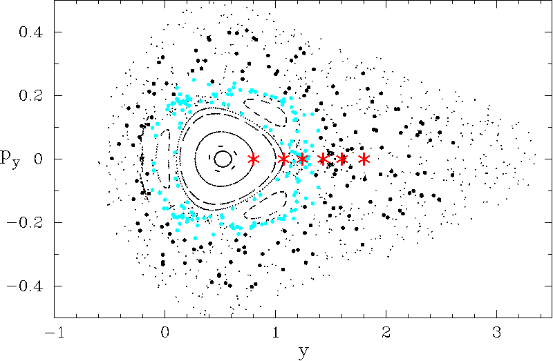
Figure 2: The Poincaré surface of section of model 2 for $E_{J}=-0.2$. The stable periodic orbit at $(y,p_{y})\approx(0.5,0)$ belongs to the main family of planar periodic orbits of the system. The 6 big asterisks indicate the initial conditions of the orbits labeled with “1” to “6” in Fig. 1b.

The six big asterisks along the $p_{y_{0}}=0$ axis with $0.8\leq y\leq 1.8$ are, from left to right, the initial conditions of the orbits “1” to “6” indicated in Fig. 1b. The evolution of the morphologies and of the quantity $\log_{10}$(GALI₂) for these orbits within $t_{1}=1$ Gyr and $t_{2}=10$ Gyr is given in Fig. 3.

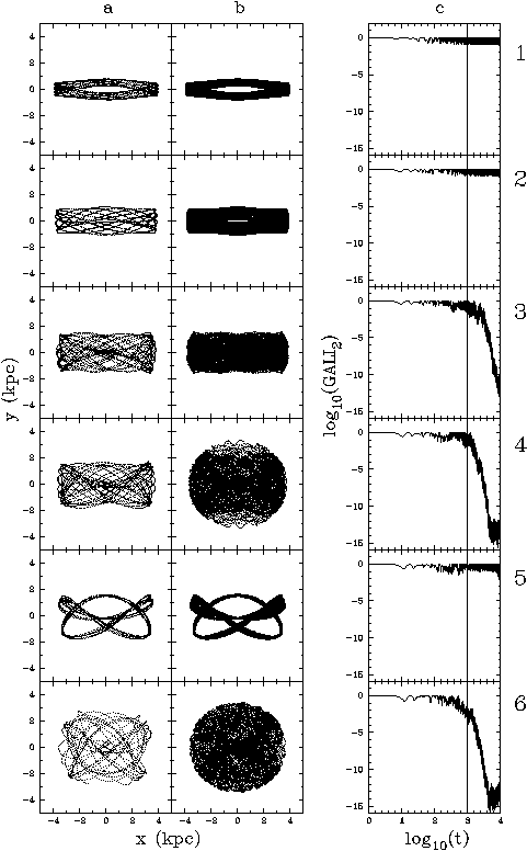
Figure 3: The six orbits with initial conditions indicated in Fig. 1b (“1” to “6”) and in Fig 2 (asterisks). Each row refers to the orbit mentioned at its right hand side. The columns (given above them) show: (a) The morphology of the orbit within $t_{1}=1$ Gyr, (b) The morphology of the orbit within $t_{2}=10$ Gyr, (c) The evolution of $\log_{10}$(GALI₂) within $t_{2}=10$ Gyr. The vertical line indicates the location of the 1st Gyr.

Orbit “1”, with $y_{0}=0.8$ (the lowest initial condition indicated with “1” in Fig. 1b) corresponds to the left asterisk in Fig 2. From its location in the surface of section we can see that it belongs to an invariant curve on the stability island around the stable representative of the main family of periodic orbits and close to it. At this energy the stable periodic orbit is a typical x1 ellipse. The quasi-periodic orbit we study has a morphology that can be vaguely described as a “thick” ellipse (panels a and b in row “1” in Fig. 3). Since it is a regular orbit $\log_{10}$(GALI₂) fluctuates close to 0 (panel c in row “1”) as expected.

Orbit “2” has $y_{0}=1.07$ and belongs also to an invariant curve. The invariant curve around orbit “2” is very close to the last KAM (Kolmogorov-Arnold-Moser) curve (see e.g. Contopoulos, 2002), of the main stability island of Fig 2. As we observe in panel (c) of the second row of Fig. 3, also in this case $\log_{10}$(GALI₂) fluctuates close to 0. The morphology of the orbit is boxy (panels a and b for “2”). However, we observe that even after integration time that corresponds to 10 Gyr there is a central region that is not visited by the orbit.

The next orbit, “3” (with $y_{0}=1.24$), gives the gray (light blue in the on-line version), heavy consequents in Fig 2. For most of the integration time these consequents are trapped around three stability islands located just beyond the invariant curve of orbit “2”. However, close to the end of the integration time, orbit “3” starts diffusing in the larger chaotic sea surrounding the region with the stability islands. Thus, it is a typical sticky orbit. The quantity $\log_{10}$(GALI₂) is very close to 0 during the first Gyr, reaching $-1$ close to the end of this time period (cf. location of vertical line in panel c in the third row in Fig. 3). Beyond that time and up to 10 Gyr it clearly decreases revealing the chaotic character of the orbit (panel c in the third row). The morphology of the orbit is boxy both for 1 as well as for 10 Gyr (panels a and b in row “3”). Diffusion in configuration space is observed only during the time the consequents start visiting all the available space in the surface of section. However, in Fig 2 we see that the light blue dots remain confined in a specific region. In panel (a) we observe that we have the formation of an X feature inside the box. The feature exists also in panel (b) of row “3”. We find that an orbit sticky to the stability island of an x1 periodic orbit has a boxy morphology with an X embedded in it. Thus, we have in this case the formation of a boxy orbit supporting an X feature on the galactic plane by means of the dynamical mechanism described by Tsigaridi & Patsis (2015).

The orbit with $y_{0}=1.43$ (4th asterisk from left in Fig 2) starts in the chaotic sea. Its consequents are drawn with heavy black dots in the surface of section. We observe that they are distributed in a larger region than the consequents of orbit “3”, while they almost do not visit the region occupied by the light blue/gray consequents. For 1 Gyr it also supports a boxy bar with an X feature as orbit “3” (panel a in the 4th row of Fig. 3) having also a rather regular behavior with $\log_{10}$(GALI₂) close to 0 (panel c, before the vertical line for “4”). However, for larger time, $\log_{10}$(GALI₂) decreases abruptly reaching smaller values than the case of orbit “3” (cf. panels c in 3rd and 4th row) and, contrarily to orbit “3”, has a chaotic morphology (panel b in “4”). We also observe that for orbit “3”, after 10 Gyr $\log_{10}$(GALI${}_{2}\approx-12$), while this happens already at $t\approx$ 5000 for orbit “4”.

Moving along the the $p_{y}=0$ axis towards larger $y$ in Fig 2, we enter a zone occupied by barely discernible stability islands. Without going into details for the periodic orbits we find there, we just mention that in the region there is a periodic orbit of multiplicity 6. This region corresponds to the white stripe below the arrow labeled with “6” in Fig. 1b. Orbit “5” ($y_{0}=1.6$) is almost on the invariant curves of the 6-ple orbit. The $\log_{10}$(GALI₂) index points to a regular orbit (panel c in row “5” of Fig. 3), which is in agreement with the morphologies after 1 and 10 Gyr as we can observe in panels a and b in “5” respectively. Actually this is also a sticky orbit whose chaotic nature will be revealed for $t>10$ Gyr, as towards the end of the integration we can observe a gradual decrease of the $\log_{10}$(GALI₂) quantity.

Finally, starting with $y_{0}=1.8$ (orbit “6”) we find a chaotic orbit (scattered small dots in Fig 2). The morphologies in panels (a) and (b) in the 6th row of Fig. 3 and the corresponding $\log_{10}$(GALI₂) index (panel c) are in agreement with the chaotic nature of the orbit.

As we observe in column a of Fig. 3, within $t_{1}=1$ Gyr the orbits “1” to “5” evidently support some structure. Only orbit “6” has a well developed chaotic character. For larger time, $t_{2}=10$ Gyr, besides orbit “6”, also orbit “4” has a chaotic morphology (panels b in “4” and “6” in Fig. 3). The boxy orbital structures that we are looking for are not encountered in all structure supporting orbits. The regular orbits “1” and essentially “5” belong to invariant curves close to the initial conditions of the periodic orbits and their morphology reflects to a large extent their morphology. Clear boxiness appears in orbits “2” and “3”. They are located in the outermost parts of the stability island of the main periodic orbit (orbit “2”) and in the sticky region around it (orbit “3”) respectively, as we can observe in Fig. 2. Their regular and sticky behavior is reflected also to their $\log_{10}$(GALI₂) index within $t_{2}=10$ Gyr (panels c of “2” and “3” in Fig. 3). The chaotic orbit “4” has a morphology similar to “3” only during the first Gyr of integration. This result is in agreement with the result of Tsigaridi & Patsis (2015), namely that boxiness in face-on views of bars at a given energy is introduced by orbits at the critical area close to the last KAM curve around the stable x1 orbit. They can be either on the regular or sticky side. In the latter case we have also the appearance of an embedded X feature.

In order to demonstrate the relation between boxiness of the orbits and their location close to the borderline between order and chaos, we considered five more orbits in this zone at various energies. These are the orbits presented in Fig. 4.

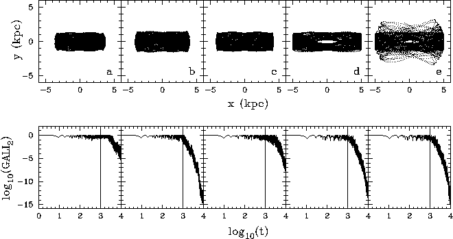
Figure 4: Five orbits with boxy character on the equatorial plane of the model of snapshot 2. Their location on the $(E_{J},y_{0})$ diagram are denoted with heavy light gray (yellow in the on-line version) dots in Fig. 1b. They are: (a) $(-0.206,1.17)$, (b) $(-0.195,1.19)$, (c) $(-0.18798,1.23)$, (d) $(-0.17,1.35)$ and (e) $(-0.162,1.27)$. All of them are sticky to the stability islands of the stable representative of the main family of periodic orbits of the system. Below its panel of the first row is given the corresponding GALI₂ index up to 10 Gyr. The vertical line indicates the location of the 1st Gyr.

All of them are sticky, located inside the dark area, but close to the borderline between white and dark (blue in the on-line version) regions in Fig. 1b. They are indicated with heavy light gray (yellow in the on-line version) dots at the energies: $E_{J}=-0.206,-0.195,-0.18798,-0.17$ and $-0.162$. Their initial $y_{0}$ values are respectively 1.17, 1.19, 1.23, 1.35 and 1.27 (always with $p_{y_{0}}$=0). In Fig. 4 we give them successively from left to right with increasing energy. Below each panel with the orbit in the $(x,y)$ plane we give its $\log_{10}$(GALI₂) index. As GALI₂ shows, all five orbits manifest their chaotic nature at times larger than 1 Gyr (indicated in all lower panels with a vertical line). Orbits in Fig. 4a to d, remain confined in the configuration space until the end of the integration time, i.e. for 10 Gyr. The orbit in Figs. 4e, at the largest energy, is more chaotic. It reaches a smaller $\log_{10}$(GALI₂) value at time 10 Gyr, while, close to the end of its integration time, it starts exploring larger regions in the configuration space. However it also has a boxy morphology within time corresponding to about 1 Gyr.

The above results point out that in order to find orbits on the equatorial plane that support boxy features in the bar of the model we have to consider initial conditions close to the borderline between order and chaos in Fig. 1. This happens not just close to a specific resonance. We find such orbits at all energies where exist x1 periodic orbits matching the size of the bar. The regions, where one should look for candidate orbits supporting boxy features in the models, are of those which still appear white after 1 Gyr of integration in Fig. 1a and are found being marginally inside the chaotic region in Fig. 1b, i.e. have developed a chaotic character in time $1<t<10$ Gyr.

4.1.2 Snapshot 3, t=7.0 Gyr

Then we repeat the same analysis for the model of snapshot 3. Figure 5, like Fig. 1, gives colour-coded the $\log_{10}$(GALI₂) quantity in a $(E_{J},y_{0})$ diagram, however this time only for $t_{2}=$ 10 Gyr. Boxy orbits are again found at the border line between order

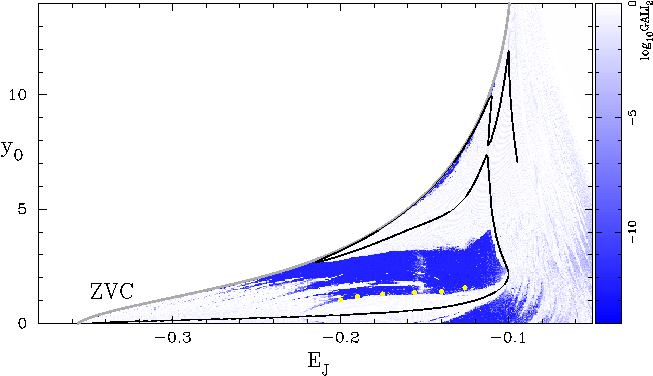
Figure 5: The chaoticity of the planar orbits on the equatorial plane of model “3”. The drawn lines and the given colors are as in Fig. 1, which is the corresponding figure for model “2”. Here we calculate $\log_{10}$(GALI₂) for $t_{2}=$ 10 Gyr. The six heavy, light gray (yellow in the online version), dots indicate the initial conditions of the boxy orbits we present in Fig. 6.

and chaos. We present six of them in Fig. 6. Their locations in Fig. 5 are at $(E_{J},y_{0})=(-0.2,1.03),(-0.19,1.19),(-0.175,1.3),(-0.156,1.35)$, $(-0.14,1.4)$ and $(-0.126,1.57)$. The time evolution of the quantity $\log_{10}$(GALI₂) below each panel with the morphology of the orbit in Fig. 6, implies that the presented orbits are sticky. them remain confined in the For $t<t_{1}=1$ Gyr these orbits can hardly be distinguished from regular orbits. We pay special attention to the orbits of panels (b) and (c) that we present in two different time windows and so they are labeled b1, b2 and c1, c2 respectively. In the first time window, which is larger than 1 Gyr, we plot the orbits for the time they are retaining its boxiness, while for the second one we plot the orbits as they appear after being integrated for $t_{2}=$10 Gyr. We observe that the orbit in b1 is boxy and harbors evidently an X structure. However, within 10 Gyr it shows a strongly chaotic character. Its morphology in the configuration space is chaotic (panel b2) and GALI₂, below it, has a steep gradient downwards reaching values close to $10^{-14}$. We encounter a similar evolution in the orbit described in panels c1 and c2. In this case the orbit remains confined in the configuration space for more than 3 Gyr and then expands into a larger region of the configuration space, without however visiting for time 10 Gyr all the allowed space.

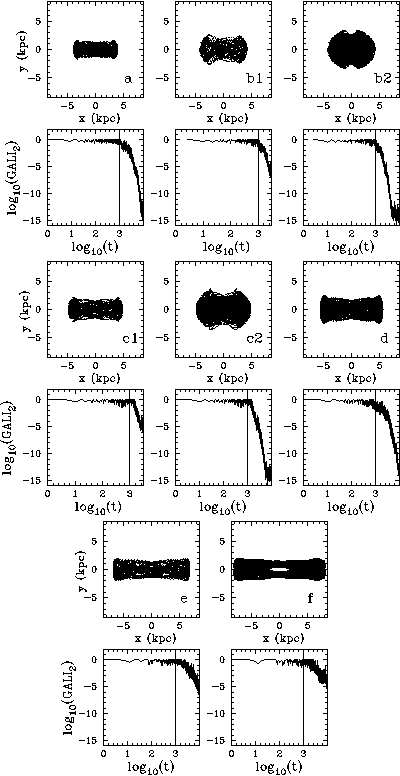
Figure 6: Six orbits with boxy character on the equatorial plane of the model of snapshot 3. Their location on the $(E_{J},y_{0})$ diagram are denoted with heavy light grey (yellow in the on-line version) dots in Fig. 5. They are: (a) $(-0.2,1.03)$, (b) $(-0.19,1.19)$, (c) $(-0.175,1.3)$, (d) $(-0.156,1.35)$, (e) $(-0.14,1.4)$ and (f) $(-0.126,1.57)$. For orbits in (b) and (c) we give their morphology in two different time windows (b1, b2 and c1, c2 respectively). All of them are sticky to the stability islands of the stable representative of the main family of periodic orbits of the system. Below each labeled panel is given the corresponding GALI₂ index up to 10 Gyr. The vertical line indicates the location of the 1st Gyr.

We also note that the boxy orbits presented in Fig. 6 have along the x=0 axis a clear $|y_{min}|$ value that gives them a bow-like shape, something that has its counterpart in the shape of the $N-$body bar in the MM models (cf. figure 1, third panel from left, in MM). This will be further discussed also in Sect. 5.

4.1.3 Snapshot 4, t=11.2 Gyr

Finally we repeat the same analysis for the last snapshot of the MM paper. The colour-coded $(E_{J},y_{0})$ diagram for this case is Fig. 7.

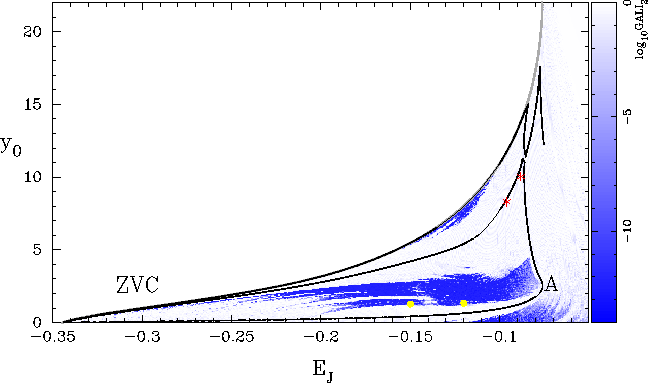
Figure 7: The chaoticity of the planar orbits on the equatorial plane of model “4”. The drawn lines and the given colors are as in Fig. 1. Here we calculate $\log_{10}$(GALI₂) for $t_{2}=$ 10 Gyr. The two heavy, light gray (yellow in the on-line version), dots indicate the positions of orbits (a) and (b) in Fig. 8, while the two asterisks, those of orbits (c) and (d) in the same figure.

This is a very slowly rotating model with $R=2.87$ and corotation at 22.89 kpc. As we can see, the loop of the characteristic of the central family is huge. The characteristic increases monotonically until point A and then turns backwards. The branch that goes back to the left reaches the minimum $E_{J}$ of the ZVC. Then it turns back again towards corotation, being essentially on the ZVC. The loop almost closes as the two parts of the characteristic come very close at about $E_{J}=-0.09$. Bar supporting orbits on the equatorial plane can be found only in the lowest branch of the characteristic, while there is a large amount of almost circular and stable orbits (practically white regions for $y_{0}>5$ in Fig. 7) that populate the extended disk region between the end of the bar and corotation (cf. figure 1, right panel, in MM). Four typical orbits for this model are given in Fig. 8. Their locations in the $(E_{J},y_{0})$ diagram are denoted with heavy light gray (yellow in the on-line version) dots and with asterisks in Fig. 7. They are at: (a) $(-0.15,1.27)$, (b) $(-0.12,1.33)$ (heavy dots), (c) $(-0.096,8.292)$, (d) $(-0.088,10.032)$ (asterisks).

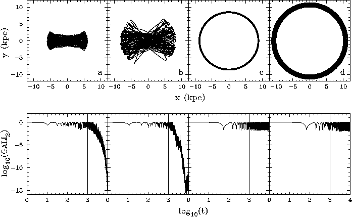
Figure 8: Four orbits on the equatorial plane of the model of snapshot 4. Their location on the $(E_{J},y_{0})$ diagram are denoted with heavy light grey (yellow in the on-line version) dots and asterisks in Fig. 7. They are: (a) and (b) the orbits with the heavy dots located at $(E_{J},y_{0})=(-0.15,1.27)$ and $(-0.12,1.33)$ respectively and (c) and (d) the orbits with the two asterisks at $(-0.096,8.292)$ and $(-0.088,10.032)$ in Fig. 7. Below each labeled panel is given the corresponding GALI₂ index up to 10 Gyr. The vertical line indicates the time corresponding to the 1st Gyr.

The accumulation of a large number of almost circular orbits for $y_{0}$ initial conditions beyond those of the bar supporting orbits and the shape of the characteristic with the almost closed loop, favor the formation of rings surrounding the bar by means of a dynamical mechanism similar to the one that led to the formation of the ring in the model of Tsigaridi & Patsis (2015).

4.2 Vertical perturbations

Until now we have seen that a set of planar orbits with boxy morphology can be found close to the border line between order and chaos above the characteristic of the central family of periodic orbits, as this is determined by the GALI₂ index in the $(E_{J},y_{0})$ diagrams. Now we will examine how the morphology of these orbits changes if we perturb them vertically by adding a $p_{z_{0}}\neq 0$ to their initial conditions. This means that the orbits we present in this section have initial conditions $y_{0}$ and $p_{z_{0}}\neq 0$, while $z_{0}$ and $p_{y_{0}}=0$. Hereafter, when we give the initial conditions of an orbit, we will mean the non-zero ones, if not otherwise indicated.

For 3D orbits their regular or chaotic character cannot be easily depicted on a single diagram, since we deal in general with four initial conditions. Considering an orbit, the monotonic variation of a single initial condition may lead to a non-monotonic succession of regular and sticky chaotic orbits. It is not easy to know in a 4D space whether the deviation from the initial condition of a torus will bring an orbit in a chaotic sea or closer to an invariant torus around another stable periodic orbit. However, we realized that for all planar boxy orbits we started increasing their $p_{z_{0}}$ coordinate, we could find a $\Delta p_{z}$ range for which the 3D orbits retained their boxy character. The variation of the GALI₂ index with time was similar to that of the boxy 2D orbits. This led to the conclusion that the building blocks not only for 2D, but also for 3D boxy structures in real galaxies can be either regular orbits on the most remote tori around stable periodic orbits, or orbits sticky to them. The latter orbits are strictly speaking chaotic, but their sticky character keeps them confined in particular regions of the phase space for sufficiently long times. This way they can support a given morphology.

Below we give some typical examples of 3D boxy orbits, or, in other words, orbits with three boxy projections in the configuration space. In Fig. 9 we present six orbits from the model of snapshot 2. The panels of each row refer to the same orbit. A number that refers to each orbit and helps us in the description, is given at the right hand side of each row. In column (a) we give the face-on views, in (b) the side-on view, in (c) the end-on one and finally in (d) the evolution of GALI₂ in a log-log plot as in the previous figures.

Figure 9: 3D orbits associated with 3D boxy structures in the model of snapshot 2. Orbit “4” has a side-on profile similar to x1v2 orbits, while all the rest have three boxy projections. Orbits “1”, “3”, “4” and “5” harbour an X feature in their face-on projections. The GALI₂ evolution indicates the sticky character of the orbits “2” to “6”, while “1” is regular. The units on the axes of the three first columns are in kpc.

In general, by starting from a planar orbit and adding $p_{z}$ we have the following possibilities: 1. We will either reach a torus around x1, or 2. a torus around a stable 3D family bifurcated from x1, or 3. a chaotic zone between the two sets of tori, or finally 4. we will enter a chaotic zone (see Patsis & Katsanikas, 2014a, and Patsis & Harsoula 2017 – in preparation). The result depends both on the energy of the orbit and the $p_{z}$ initial condition. The energy will determine the available resonant families of periodic orbit existing (their number increases with $E_{J}$), while $p_{z}$ will decide about the location of the orbit in the phase space. In the present paper we are interested just in pointing out that there are vertical perturbations that support the 3D boxy character. The planar orbits we start from have to be sought along the lines we find the 2D boxy orbits in the $(E_{J},y_{0})$ diagrams. In Fig. 9, the orbits in the four first rows are at the same energy we have the $(y,p_{y})$ surface of section in Fig. 2, i.e. for $E_{J}=-0.2$. The orbits “1” and “2” have $y_{0}=1.07$, which would be an initial condition on an invariant curve around x1 in the $(y,p_{y})$ Poincaré surface of section (Fig. 2) if we had $p_{z}=0$. However, orbit “1” is perturbed by $p_{z}=0.15$ and orbit “2” by $p_{z}=0.2$. In both cases the orbits form boxes in all three projections. The side-on and end-on morphologies clearly support peanut-shaped structures. The GALI₂ evolution of orbit “1” (panel d) indicates that it is a regular orbit, while that of orbit “2” points to a sticky one. The next orbit, perturbed by $p_{z}=0.085$, has $y_{0}=1.24$, i.e. in the $(y,p_{y})$ Poincaré surface of section in Fig. 2 corresponds to the sticky orbit plotted with the heavy gray/light blue consequents. Again in this case the 3D boxy character is retained, however this time the vertical perturbation is smaller. For the same energy we give an example of an orbit with $y_{0}=1.19$ and $p_{z}=0.165$, which is orbit “4” in Fig. 9. If $p_{z}=0$ the orbit would be a sticky to x1 orbit. Now it is sticky again, but its morphology clearly resembles the morphology of the x1v2 family, which is bifurcating, usually as unstable, at the vertical 2/1 resonance (Skokos et al., 2002a). This can be seen in panel (b) of row “4” in Fig. 9. Strictly speaking this side-on profile is not boxy. Nevertheless it has a shape similar to the one of the two main vertical bifurcations of x1. Considering several orbits like this in different energies will lead to a boxy profile. The orbits “5” and “6” are in nearby energies and have similar morphologies and evolution of GALI₂ as the previous ones. Orbit “5” is at $E_{J}=-0.206$ with $y_{0}=1.17$ and $p_{z}=0.162$, while orbit “6” at $E_{J}=-0.195$ with $y_{0}=1.19$ and $p_{z}=0.15$.

An interesting result is that the sticky 3D boxy orbits in many cases harbor an X feature in their face-on projections (column a). This is conspicuous in orbits “3”, “4” and “5”, as well as in the regular orbit “1”. This is in agreement with the result of Patsis & Katsanikas (2014b) who suggest that sticky boxy orbits at the immediate neighborhood of the vertical 2:1 resonance have embedded X features in their face-on projections. The property of stickiness was also the reason for the appearance of an X inside the bars of the 2D barred-spiral models in Tsigaridi & Patsis (2015). The same analysis led to similar results in the cases of the two other models considered here as well. In Fig. 10 we present some typical orbits for the model of snapshot 3. Again here, double boxiness with an X feature embedded in the boxy face-on projection is found by perturbing boxy planar orbits in the z direction by $p_{z}$. This is given in orbit “1”, which is for $E_{J}=-0.156$, $y_{0}=1.35$ and $p_{z}=0.09$. In Fig. 6d we have given the corresponding orbit with $p_{z}=0$. As the orbits “2” and “3” show, the stable 3D families (x1v1 and x1v1^′ in the notation of Skokos et al., 2002a) bifurcated from x1

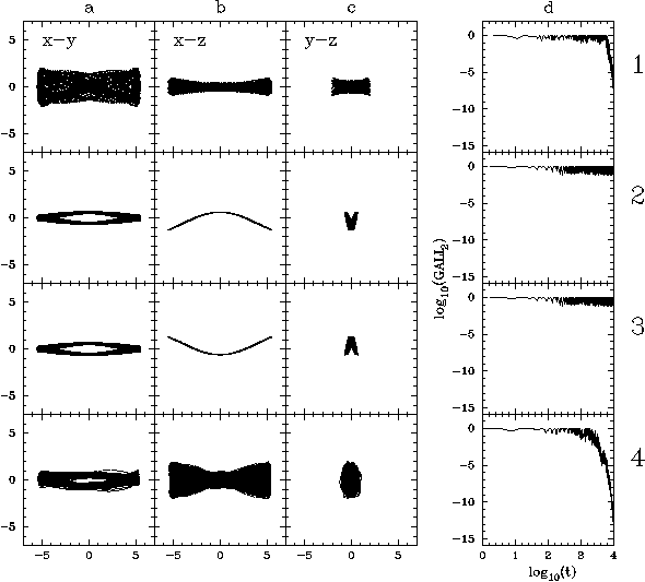
Figure 10: Orbits in the model of snapshot 3. “1” Sticky orbit with a boxy 3D structure and an X feature embedded in the face-on projection, “2” and “3” frown and smile regular 3D orbits on x1v1 tori, “4” a sticky orbit that changes its face-on elliptical morphology becoming boxy as soon as it abandons its regular behavior. The units on the axes of the three first columns are in kpc.

at the vertical 2/1 resonance, do exist in the model. In order to track them we perturbed in the vertical direction the z coordinate, while we put the initial condition $p_{z}=0$. The initial conditions of the two orbits are $E_{J}=-0.156$, $y_{0}=0.7$ and $z=0.63$ (orbit “2”) and $E_{J}=-0.156$, $y_{0}=0.7$ and $z=-0.63$ (orbit “3”) respectively. Their morphology indicates that they belong to invariant tori in the immediate neighborhood of x1v1 (Patsis & Katsanikas, 2014b). This is consistent with the evolution of their GALI₂ index in panels (d). By means of such orbits we can construct a sharp X-shaped side-on profile, having however an elliptical face-on morphology. A nice example is given with orbit “4” with non-zero initial conditions $E_{J}=-0.156$, $y_{0}=0.7$ and $p_{z}=0.303$. This is a sticky orbit (see panel d). As long as it has a regular character, the orbit supports an elliptical face-on morphology. However, when it starts diffusing in the configuration space it tends to obtain a boxy structure (panel a).

Finally in Fig. 11 we give an example of an orbit from the model of snapshot 4, that reproduces the main morphology we want to underline that exists in our models. Namely, it is a sticky orbit with all its projections boxy, while in its face-on projection it is discernible an X feature. The initial conditions of the orbit are: $E_{J}=-0.15$, $y_{0}=1.27$ and $p_{z}=0.07$.

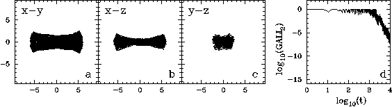
Figure 11: A 3D boxy orbit in the model of snapshot 4. It is sticky (panel d) and reproduces the X feature in its face-on projection (panel a). The units on the axes of the three first panels are in kpc.

The process for finding 3D double boxy orbits by perturbing 2D boxy ones can be applied at all energies, for which we could find x1 orbits supporting the size of the $N$-body bar in the models. However, as $E_{J}$ increases and we approach corotation, the structure of phase-space becomes more complicated, due to the presence of more families of periodic orbits introduced in the system at successive resonances (Skokos et al., 2002a). The monotonic variation of an initial condition (e.g. $p_{z}$) may lead either to quasi-periodic orbits around stable periodic orbits and to the sticky to them chaotic orbits, or to direct diffusion in the chaotic sea. This happens in general in a nonmonotonic way. As an example, we give in Fig. 12 the orbit of the model of snapshot 3 with $(E_{J},y_{0})=(-0.14,1.4)$, given in Fig. 6e, perturbed by $p_{z}=0.038,0.039$ and $0.040$.

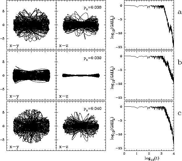
Figure 12: The planar orbit presented in Fig. 6e perturbed by $p_{z}=0.038$ (a), $0.039$ (b) and $0.040$ (c). In (a) and (c) the orbits diffuse in configuration space, while in (b) the orbit has for more than 3 Gyr a double boxy character.

We observe that for $p_{z}=0.038$ the orbit clearly diffuses in the configuration space, for $p_{z}=0.039$ has a double boxy character for more than 3 Gyr before starting diffusing in the chaotic sea (the quantity $\log_{10}$(GALI₂) $\lessapprox-10$ at $t=10$ Gyr) and for $p_{z}=0.040$ we have again a practically chaotic orbit.

In order to demonstrate the fact that at energies where several families of 3D periodic orbits co-exist, different perturbations of the planar orbits may lead us to different boxy configurations, we present in Fig. 13 the planar orbit of the model of snapshot 2, given in Fig. 4e. It has $(E_{J},y_{0})=(-0.162,1.27)$. In (a) $p_{z}=0.016$. The orbit, being initially boxy on the equatorial plane, has a narrow side-on profile. This morphology lasts for more than 3 Gyr. Then the orbit occupies a larger volume in phase space. However, it retains a less confined, but boxy, character in its face-on view, while in the side-on view its morphology resembles the one encountered in orbits close to the stable “frown” and “smiles” periodic orbits.

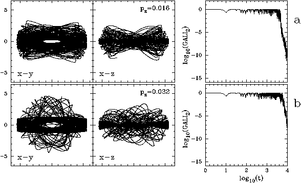
Figure 13: The planar orbit presented in Fig. 4e ($(E_{J},y_{0})=(-0.162,1.27)$) perturbed by $p_{z}=0.016$ (a) and $p_{z}=0.032$ (b). The orbit has initially a x1v3 side-on profile, while for longer times its morphology is different in each case.

For $p_{z}=0.032$ (Fig. 13b) the orbit remains boxy on its face-on view for even longer time than for $p_{z}=0.016$, but then diffuses in phase space and does not have any particular morphology in either projections. The side-on views of the orbits in both cases of Fig. 13, clearly indicate that they have been trapped close to a x1v3 periodic orbit, which is bifurcated at the 3:1 vertical resonance (Patsis et al., 2002). It is worth to underline that the side-on profiles of the double boxy orbits in which a morphology of a higher order $n:1$ resonance may be identified are in general narrower as we approach corotation, in agreement with the profile of the corresponding periodic orbits found in Patsis et al. (2002).

Before closing, we want to add a comment on the general morphology of the three models from the MM simulation and especially in the one that appears in snapshots 3 and 4 (cf. figure 1 in MM). This morphology is one of a bar surrounded by a ring, with the areas on the sides of the bar being rather depleted from particles. Beyond this central structure there is a disk without any special feature. The bar and ring morphology could easily correspond to that of a bar with an inner ring (Buta & Combes, 1996). However, in this particular case corotation is far away, so the question that arises is what is the orbital content behind this structure in the model. The orbits that we have presented so far support a bar of the size of the bars in the MM $N$-body snapshots. The folding of the characteristic provides appropriate round orbits with the right dimensions to support the ring.

Focusing on the model of snapshot 4, we can see that the sticky bar-supporting orbits have face-on projections that reinforce a bar structure with two minima along the minor axis, giving it a bow-like or peanut-like form, however on the equatorial plane of the model in this case (Fig. 11a). The planar, sticky, boxy orbits have a similar shape (Fig. 8a). The corresponding MM model has this morphological feature as well. At larger energies one can find in the plane some tumbling bar-supporting orbits (see Fig. 8b). However, even by considering these orbits to be among those that populate the model, the areas on the sides of the bar remain rather empty. Finally, not only the presence of the circular orbits with the right dimensions, but also the regression of the characteristic and the following continuation of the curve forwards, i.e. towards corotation, favors the accumulation of round orbits around the bar. This folding of the characteristic brings in the system twice as much stable circular periodic orbits as in the rest of the energies and this supports the formation of a circular ring at a certain distance. All these are summarized in Fig. 14, where we combine the orbits of Fig. 8 in order to reproduce the main morphology of the $N$-body MM model. We also plot two circular periodic orbits as a reference to the dimensions of the ring. The initial conditions for the two periodic orbits are: $E_{J}=-0.0961538$, $y_{0}=8.49173$ and $E_{J}=-0.0898683$, $y_{0}=10.0141$, respectively. Fig. 14 is by no means the result of a self-consistent Schwarzschild-type model. It just shows that in the snapshot “4” model, exist orbits that can reproduce the morphology of the corresponding MM $N$-body model.

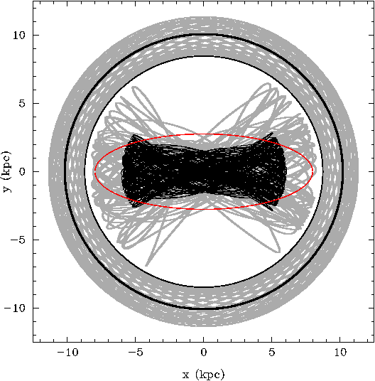
Figure 14: The set of the four non-periodic orbits of the model for snapshot 4 that are depicted in Fig. 8 reproduce the basic morphological features of the corresponding MM model. Two circular periodic orbits at close-by energies are also plotted. A ringed bar morphology is formed, however away from corotation, which in this case is at 22.89 kpc. The red ellipse indicates the bar in the MM snapshot.

4.3 Fast rotating bars

In the present paper we studied orbital boxiness in the MM models, all of which have slow rotating bars. We have found that boxiness is a property associated with the presence of x1 orbits supporting the bar. This is not related with the pattern speed of the model per se. However, in slow rotating models like the models of the MM simulations, there are a lot of non-bar-supporting orbits between the end of the bar and corotation. These are the circular orbits. Contrarily, in fast rotating bars one can find bar supporting elliptical x1 orbits almost all the way from the center of the system to corotation.

In order to examine the dependence of the results on the pattern speed a systematic study with models of bars rotating in a range of $\Omega_{b}$ is needed. This is not done in the present paper. Nevertheless, we considered the potential of one of the models (model of snapshot "3") with a higher pattern speed, so that we obtained a ratio $R_{CR}/\alpha_{b}=1.1$. This model is not the result of an N-body simulation. It has been used just for studying the orbital behavior of bar supporting orbits close to corotation.

We found again in this case that the 2D orbits at the borders of the stability islands of x1 were boxy and we could find 3D boxy orbits by perturbing them in the vertical directions within a certain $\Delta p_{z}$ range. So the rule in principle applies also in the case of bar supporting orbits close to corotation. However, we have to note that the planar boxy bar-supporting orbits we could find close to corotation on the plane were like the orbit "1" in Fig. 3 and not like orbit "3" of the same figure. In other words at their apocentra the segments that were parallel to the minor axis of the bar were relatively small. On the $(y,p_{y})$ Poincaré sections we found more islands of orbits of higher multiplicity than in Fig. 2. Many of them surround the stability islands of x1 and this affects the shape of the sticky orbits in the region. Also the $\Delta p_{z}$ range for which we could find double boxy orbits was much smaller. The 3D double boxy bar-supporting orbits remained confined close to the equatorial plane. We could find orbits with boxy edge-on profiles away from the equatorial plane, but their face-on projections did not support the bar.

In conclusion: The mechanism applies independently of the pattern speed value. However it applies more efficiently away from corotation. If a bar stops away from corotation (as in the slow rotating models) then almost all of it can be considered as a double boxy structure. In fast rotating models the 3D double boxy part can be found pronounced in the inner parts of the bar.

5 DISCUSSION AND CONCLUSIONS

The orbital analysis we present in this paper, suggests a recipe for building two- and three-dimensional boxy structures in rotating bars. The basic idea is the following: Let us start with the planar backbone of periodic orbits for building a bar, namely with the well known x1 family. However, instead of populating the model with regular quasi-periodic orbits encountered in the immediate neighborhood of the periodic orbit, we consider either periodic orbits close to the last KAM or, more efficiently, the sticky orbits that surround the islands of stability, as they appear in the surfaces of section. The selection of these orbits secure a boxy morphology on the plane.

In a 3D model, when we eject out of the plane particles that follow the 2D boxy orbits by adding a $p_{z}\neq 0$ perturbation, we find that there is always a $\Delta p_{z}$ range of perturbations for which all three projections of the 3D orbits are boxy. A remarkable property of these sticky boxy orbits is the formation of an X feature embedded in the bar in the face-on projections.

In several cases the side-on views had a peanut-shaped morphology. However, it is beyond the scope of the present paper to attribute specific orbits, or sets of orbits to the observed peanut shapes encountered in edge-on galaxies or snapshots of $N$-body models. This was investigated thoroughly in Patsis & Katsanikas (2014b). In this study we emphasize that as long as we have the usual ellipses of the x1 family (or the x1-tree in 3D models according to Skokos et al., 2002a) in a rotating bar, we can find a class of boxy 2D and 3D orbits. They are sticky chaotic orbits as their GALI₂ index indicates and they can support the bar, or a part of the bar, for many Gyr.

Observational features that can be reproduced by using such orbits as building blocks, can firstly be the boxy- or peanut-shaped bulges in the central parts of the bars. In these cases in the face-on views of the galaxies, we will observe boxy isophotes in their central parts, inside the bar, as in the sample of galaxies presented by Erwin & Debattista (2013). On the other hand, the present study indicates that in cases of slow rotating bars as in the MM models, the 3D boxy structure may constitute a major part of the bar. The presence of the X feature in the face-on views of the orbits, as well as the presence of a ring surrounding the bar, raises the question whether a dynamical mechanism as the one proposed by Tsigaridi & Patsis (2015), acts in galaxies like IC 5240 presented in Buta et al. (2007).

Closing, we enumerate below our conclusions:

1. In models where the family of x1 ellipses exists in the MM models we can find a class of sticky chaotic orbits with a 2D and/or 3D boxy structure. The shape of these orbits, after integrating them for 10 Gyr and the evolution of their GALI₂ index show that they can be used as building blocks for structures that last for several Gyr. They exist in a large range of $E_{J}$’s.

2. 2D non-periodic boxy orbits can be found on the outermost invariant curves around x1 on a surface of section, or in regions in the immediate neighbourhood of the stability islands. We found them in all $E_{J}$’s we encounter x1 periodic orbits that do not exceed the size of the $N$-body bar.

3. For finding 3D orbits with boxy morphology in both face-on and edge-on views, one has to perturb in the vertical direction the boxy planar orbits. There is always a $\Delta p_{z}$ interval in the initial conditions of the perturbed, initially planar, orbits in which the 3D orbits will have a boxy structure. These are 3D sticky chaotic orbits. Their face-on projections are different from those of the quasi-periodic orbits close to x1 and its 3D bifurcations, at all $E_{J}$’s we find them.

4. In the face-on projections of these sticky boxy orbits we find the formation of an X embedded in the boxy structure.

5. Such orbits can be used to construct models with boxy isophotes inside the face-on views of the bars. The areas of the boxy isophotes in these cases correspond to the extent of the edge-on boxy bulges, in agreement with the result of Patsis & Katsanikas (2014b).

6. According to our analysis, the degree of boxiness of a bar, or of a part of it, indicates which orbits are populated. If quasi-periodic orbits in the immediate neighbourhood of the periodic orbits of the central family prevail, the face-on projections will be elliptical. On the other hand if the majority of the non-periodic orbits building the bar, or its part, are at the edges of the stability islands and/or sticky chaotic orbits next to them, then the supported shape in the face-on views will be boxy. In both cases we can have boxy edge-on profiles.

7. In the case of slow rotation, our 3D sticky, boxy orbits can build boxy bars (not just boxy features embedded in the bars). In such cases almost the whole bar is boxy. The slow rotation of the models favours the appearance of a ringed bar morphology, despite the fact that corotation is at large distances.

   On the other hand, in a fast rotating case we examined, we found that boxy bar-supporting planar orbits close to corotation had small segments parallel to the minor axis of the bar at their apocentra. By perturbing them in the vertical direction we could find boxy orbits supporting the bar confined close to the equatorial plane. In such a case double boxy structures are found mainly embedded in the bar.

References

- Athanassoula (1992a) Athanassoula, E. 1992a, MNRAS, 259, 328
- Athanassoula (1992b) —. 1992b, MNRAS, 259, 345
- Barazza et al. (2008) Barazza, F. D., Jogee, S., & Marinova, I. 2008, ApJ, 675, 1194, 0710.4674
- Benettin et al. (1980) Benettin, G., Galgani, L., Giorgilli, A., & Strelcyn, J.-M. 1980, Meccanica, 15, 9
- Binney & Tremaine (2008) Binney, J., & Tremaine, S. 2008, Galactic Dynamics: Second Edition (Princeton University Press)
- Bountis & Papadakis (2009) Bountis, T., & Papadakis, K. E. 2009, Celestial Mechanics and Dynamical Astronomy, 104, 205
- Buta & Combes (1996) Buta, R., & Combes, F. 1996, Fund. Cosmic Phys., 17, 95
- Buta et al. (2007) Buta, R. J., Corwin, H. G., & Odewahn, S. C. 2007, The de Vaucouleurs Altlas of Galaxies (Cambridge University Press)
- Capuzzo-Dolcetta et al. (2007) Capuzzo-Dolcetta, R., Leccese, L., Merritt, D., & Vicari, A. 2007, ApJ, 666, 165, astro-ph/0611205
- Carpintero et al. (2014) Carpintero, D. D., Muzzio, J. C., & Navone, H. D. 2014, MNRAS, 438, 2871, 1312.3180
- Contopoulos (1980) Contopoulos, G. 1980, A&A, 81, 198
- Contopoulos (2002) —. 2002, Order and chaos in dynamical astronomy
- Contopoulos & Grosbol (1989) Contopoulos, G., & Grosbol, P. 1989, A&A Rev., 1, 261
- Contopoulos & Harsoula (2008) Contopoulos, G., & Harsoula, M. 2008, International Journal of Bifurcation and Chaos, 18, 2929, 0802.4208
- Contopoulos & Harsoula (2013) —. 2013, MNRAS, 436, 1201
- Debattista & Sellwood (2000) Debattista, V. P., & Sellwood, J. A. 2000, ApJ, 543, 704, astro-ph/0006275
- Dehnen (1993) Dehnen, W. 1993, MNRAS, 265, 250
- Erwin & Debattista (2013) Erwin, P., & Debattista, V. P. 2013, MNRAS, 431, 3060, 1301.0638
- Eskridge et al. (2000) Eskridge, P. B. et al. 2000, AJ, 119, 536, astro-ph/9910479
- Ferrers (1877) Ferrers, N. M. 1877, Quart.J.Pur.Appl.Math., 14, 1
- Harsoula & Kalapotharakos (2009) Harsoula, M., & Kalapotharakos, C. 2009, MNRAS, 394, 1605, 1008.0493
- Harsoula et al. (2010) Harsoula, M., Kalapotharakos, C., & Contopoulos, G. 2010, in Astronomical Society of the Pacific Conference Series, Vol. 424, 9th International Conference of the Hellenic Astronomical Society, ed. K. Tsinganos, D. Hatzidimitriou, & T. Matsakos, 377
- Kaufmann & Contopoulos (1996) Kaufmann, D. E., & Contopoulos, G. 1996, A&A, 309, 381
- Knapen et al. (2000) Knapen, J. H., Shlosman, I., & Peletier, R. F. 2000, ApJ, 529, 93, astro-ph/9907379
- Machado & Athanassoula (2010) Machado, R. E. G., & Athanassoula, E. 2010, MNRAS, 406, 2386, 1004.3874
- Machado & Manos (2016) Machado, R. E. G., & Manos, T. 2016, MNRAS, 458, 3578, 1603.02294
- Manos & Athanassoula (2011) Manos, T., & Athanassoula, E. 2011, MNRAS, 415, 629, 1102.1157
- Manos et al. (2013) Manos, T., Bountis, T., & Skokos, C. 2013, Journal of Physics A Mathematical General, 46, 254017, 1208.3551
- Manos & Machado (2014) Manos, T., & Machado, R. E. G. 2014, MNRAS, 438, 2201, ADS, 1311.3450
- Manos et al. (2012) Manos, T., Skokos, C., & Antonopoulos, C. 2012, International Journal of Bifurcation and Chaos, 22, 1250218, 1103.0700
- Manos et al. (2008) Manos, T., Skokos, C., Athanassoula, E., & Bountis, T. 2008, Nonlinear Phenomena in Complex Systems, vol. 11, p. 171-176, 11, 171, ADS, nlin/0703037
- Marinova & Jogee (2007) Marinova, I., & Jogee, S. 2007, ApJ, 659, 1176, astro-ph/0608039
- Menéndez-Delmestre et al. (2007) Menéndez-Delmestre, K., Sheth, K., Schinnerer, E., Jarrett, T. H., & Scoville, N. Z. 2007, ApJ, 657, 790, astro-ph/0611540
- Miyamoto & Nagai (1975) Miyamoto, M., & Nagai, R. 1975, PASJ, 27, 533
- Muzzio et al. (2005) Muzzio, J. C., Carpintero, D. D., & Wachlin, F. C. 2005, Celestial Mechanics and Dynamical Astronomy, 91, 173
- Patsis et al. (1997) Patsis, P. A., Athanassoula, E., & Quillen, A. C. 1997, ApJ, 483, 731
- Patsis et al. (2010) Patsis, P. A., Kalapotharakos, C., & Grosbøl, P. 2010, MNRAS, 408, 22, 1009.0403
- Patsis & Katsanikas (2014a) Patsis, P. A., & Katsanikas, M. 2014a, MNRAS, 445, 3525, 1410.4921
- Patsis & Katsanikas (2014b) —. 2014b, MNRAS, 445, 3546, 1410.4923
- Patsis et al. (2002) Patsis, P. A., Skokos, C., & Athanassoula, E. 2002, MNRAS, 337, 578, ADS
- Reese et al. (2007) Reese, A. S., Williams, T. B., Sellwood, J. A., Barnes, E. I., & Powell, B. A. 2007, AJ, 133, 2846, astro-ph/0702720
- Sándor et al. (2004) Sándor, Z., Érdi, B., Széll, A., & Funk, B. 2004, Celestial Mechanics and Dynamical Astronomy, 90, 127
- Skokos (2001) Skokos, C. 2001, Journal of Physics A Mathematical General, 34, 10029
- Skokos (2010) Skokos, C. 2010, in Lecture Notes in Physics, Berlin Springer Verlag, Vol. 790, Lecture Notes in Physics, Berlin Springer Verlag, ed. J. Souchay & R. Dvorak, 63–135, 0811.0882, ADS
- Skokos et al. (2016) Skokos, C. ., Gottwald, G. A., & Laskar, J. 2016, in Lecture Notes in Physics, Berlin Springer Verlag, Vol. 915, Chaos Detection and Predictability
- Skokos et al. (2003) Skokos, C., Antonopoulos, C., Bountis, T. C., & Vrahatis, M. N. 2003, Progress of Theoretical Physics Supplement, 150, 439, nlin/0301035
- Skokos et al. (2004) —. 2004, Journal of Physics A Mathematical General, 37, 6269, nlin/0404058
- Skokos et al. (2008) Skokos, C., Bountis, T., & Antonopoulos, C. 2008, European Physical Journal Special Topics, 165, 5, 0802.1646
- Skokos et al. (2007) Skokos, C., Bountis, T. C., & Antonopoulos, C. 2007, Physica D Nonlinear Phenomena, 231, 30, 0704.3155
- Skokos & Manos (2016) Skokos, C., & Manos, T. 2016, Lecture Notes in Physics, 915
- Skokos et al. (2002a) Skokos, C., Patsis, P. A., & Athanassoula, E. 2002a, MNRAS, 333, 847, astro-ph/0204077
- Skokos et al. (2002b) —. 2002b, MNRAS, 333, 861, astro-ph/0204078
- Soulis et al. (2007) Soulis, P., Bountis, T., & Dvorak, R. 2007, Celestial Mechanics and Dynamical Astronomy, 99, 129
- Tsigaridi & Patsis (2015) Tsigaridi, L., & Patsis, P. A. 2015, MNRAS, 448, 3081, 1502.00548
- Voglis et al. (2007) Voglis, N., Harsoula, M., & Contopoulos, G. 2007, MNRAS, 381, 757
- Voyatzis (2008) Voyatzis, G. 2008, ApJ, 675, 802, ADS
- Wozniak (1994) Wozniak, H. 1994, in Lecture Notes in Physics, Berlin Springer Verlag, Vol. 430, Ergodic Concepts in Stellar Dynamics, ed. V. G. Gurzadyan & D. Pfenniger, 264
- Wozniak & Pfenniger (1999) Wozniak, H., & Pfenniger, D. 1999, Celestial Mechanics and Dynamical Astronomy, 73, 149