Evolution with mass extinction on $\mathbb{T}_{d}^{+}$

Abstract.

We propose a stochastic model for evolution through mutation and natural selection of a population that evolves on a $\mathbb{T}_{d}^{+}$ tree. We think of this model as a way of describing the evolution fitness landscape of a population. We obtain sharp and distinct conditions on the set of parameters for extinction and survival.

1. Introduction

We propose a stochastic spatial model for evolution through mutation and natural selection. The proposed model is an interacting particle system evolving on $\mathbb{T}_{d}^{+}$ (an infinite rooted tree whose vertices have degree $d+1$, except the root that has degree $d$) whose state space is $\{0,1\}^{\mathbb{T}_{d}^{+}}$. That is, the status of a vertex can be either “0” (empty) or “1” (occupied by a particle). The set of vertices that are at a distance $i$ from the root is namely the level $i$ of the tree. At time $t=0$ there is only one particle in the system, located at the root of $\mathbb{T}_{d}^{+}$. This particle will have a deterministic lifetime of length 1. During its lifetime, following a Poisson process of rate $\lambda$, it generates offspring (new particles) which will be placed randomly, one by one, on its $d$ nearest neighbours up to the time it dies or up to the event that all its nearest neighbours are occupied. In general, each particle which are placed at level $i$ of ${\mathbb{T}_{d}^{+}}$ may generate offspring according to an independent Poisson process with rate $\lambda$. These offspring will be placed randomly, one by one, at one of the $d$ nearest neighbours ($(i+1)-th$ level) up to the time their progenitor dies or up to the event that all these $d$ nearest neighbours are occupied. With respect to the death time, all individuals placed at level $i$ follow the same clock. However, this clock (of length 1) does not start to tick until their progenitors (placed at level $(i-1)$) dies out. We call this the residual lifetime. Note that while individuals placed at a given level have different lifetimes they die (and are removed) at the same time. Besides that their residual lifetime starts and ends at the same moment. We call this a mass extinction event.

We think of our model as describing the fitness landscape of a population. We consider the offspring as beneficial mutations that occurs in the population and the level where they are placed, their fitness. Here $(i)$ a mutation is not at risk while its progenitor is alive and $(ii)$ a death event at a given time, kills all the least fit mutations (particles placed at the lower level) present in the process. It combines features that have been recently explored in population evolutionary dynamics as it assumes $(i)$ the occurrence of mass extinction events that may lead all individuals of certain type in the population to extinction as in Schinazi and Schweinsberg [9] and $(ii)$ that mass extinction events kill the least fit type of individuals in the population as in Guiol et al. [3]. Figure 1.1 shows an illustration of the model on $\mathbb{T}_{2}^{+}$.

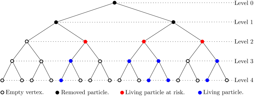
Figure 1.1. Illustration of the model on $\mathbb{T}_{2}^{+}$ with vertex depth up to 4.

Our model is a variation of the birth-and-assassination (BA) process introduced by Aldous and Krebs [1].The BA process is a variant the classical branching process. It was stated to investigate the scaling limit of a certain queuing system with blocking which appeared in database processing, see Tsitsiklis et al [7]. In the BA process the clocks that define the residual lifetime of each offspring of a particle start to tick as soon as the lifetime of that particle comes to an end, independently from each other. Another difference in BA process is that each particle which are placed at level $i$ may generate offspring according to an independent Poisson process with rate $\lambda$ and no restriction. Our model has a stronger dependence among particles lifetime, as all particles at the same level share the same clock as for the death time.

Our model is also related to spatial catastrophe models where large sets of individuals are simultaneously removed, see for example Lanchier [5] and Machado et al. [6]. We can also imagine the particles in this process as pathogens in such way that if the process dies out, the disease is defeated.

The aim of this paper is to establish the relationship between the birth and death rates in the survival or extinction of infectious process. Hence, we found conditions under which particles are eventually removed from $\mathbb{T}_{d}^{+}$.

Definition 1.1.

If all particles are eventually removed from $\mathbb{T}_{d}^{+}$ with probability 1, we say that the process dies out. Otherwise, we say that the process survives.

Let us introduce the notation $\eta_{t}\in\{0,1\}^{\mathbb{T}_{d}^{+}}$ for the status of the vertices in terms of occupation at time $t$ and $|\eta_{t}|$ for the amount of particles present at time $t$. By coupling arguments, one can see that the probability of survival is a non-decreasing function of $\lambda$. This is so because more births (greater $\lambda$) can only help survival. So we define

$$\lambda_{c}(d):=\inf\{\lambda:\mathbb{P}(|\eta_{t}|\geq 1\hbox{ for all }t\geq 0)>0\}.$$

2. Results

We prove phase transition (meaning that $0<\lambda_{c}(d)<\infty$) for this process.

Theorem 2.1.

For $d$ fixed

$$\lambda_{c}(d)=\inf\left\{\lambda:\inf_{u>0}\frac{\lambda e^{u}}{u}\left[1-\left(\frac{\lambda}{\lambda+u}\right)^{d}\right]>1\right\}.$$

If $\lambda<\lambda_{c}(d)$ then the process $\eta_{t}$ dies out. If $\lambda>\lambda_{c}(d)$ then the process $\eta_{t}$ survives.

Remark 2.2.

Let us define

$$f_{d}(\lambda):=\inf_{u>0}\frac{\lambda e^{u}}{u}\left[1-\left(\frac{\lambda}{\lambda+u}\right)^{d}\right].$$

The function $f_{d}(\lambda)$ is continuous and strictly monotone in $(0,1)$, $f_{d}(0)=0$ and $f_{d}(1)>1$. Thus, by Theorem 2.1, we have that $\lambda_{c}(d)$ is the unique solution for $f_{d}(\lambda)=1$.

Table 1 shows some numerical approximations for $\lambda_{c}(d)$.

$d$	2	3	4	5	6	7
$\lambda_{c}(d)$	0.40564	0.37596	0.36990	0.36839	0.36800	0.36792

Table 1. Numerical approximations for $\lambda_{c}(d)$.

From the fact that $\lim_{d\to\infty}f_{d}(\lambda)=e\lambda$ and adapting the proof of Proposition 3.1 in Junior et al. [4] one can see that

$$\lambda_{c}(d)\rightarrow 1/e.$$ (2.1)

3. Proofs

The proof below adapts a strategy presented in Aldous and Krebs [1] for the survival and extinction of the birth-and-assassination (BA) process. We nevertheless include all the details here for completeness.

Proof Theorem 2.1.

First, we show that, the process goes extinct with probability 1, if $\inf_{u>0}\left\{\frac{\lambda e^{u}}{u}\left[1-\left(\frac{\lambda}{\lambda+u}\right)^{d}\right]\right\}<1$.
Let $X_{i}$, $i=1,\ldots,d$, denote independent Gamma random variables with parameters $i$ and $\lambda$, respectively, and consider a random variable $W$ with probability distribution given by

$$\mathbb{P}(W\leq w)=\frac{1}{d}\left[\sum_{i=1}^{d}\mathbb{P}(X_{i}\leq w)\right],~{}w\geq 0.$$

Note that, for $u>0$,

$$\mathbb{E}\left[e^{-uW}\right] = \frac{1}{d}\left[\frac{\lambda}{\lambda+u}+\left(\frac{\lambda}{\lambda+u}\right)^{2}+\cdots+\left(\frac{\lambda}{\lambda+u}\right)^{d}\right]$$

$$= \frac{\lambda}{ud}\left[1-\left(\frac{\lambda}{\lambda+u}\right)^{d}\right].$$

In our model, each time a particle occupying a vertex at the $k$-th level of $\mathbb{T}_{d}^{+}$ has an offspring, it chooses uniformly at random a position to place its offspring among its empty neighboring vertices at the $(k+1)$-th level of $\mathbb{T}_{d}^{+}$; once no empty vertex is left all incoming particles are ignored. In the absence of any information on these births and the ordering of the occupancy of the neighboring vertices at the $(k+1)$-th level, the time which is necessary for a fixed vertex at the $(k+1)$-th level to receive an offspring of a particle on its neighboring vertex at the $k$-th level has the same distribution of a random variable $W$. To see this, note that the fixed vertex at $(k+1)$-th level is occupied by the $i$-th offspring of its neighbor at $k$-th level with probability $1/d$. The time for this to occur has Gamma distribution with parameters $(i,\lambda)$. Of course, such ‘virtual’ births only become ‘real’ ones, if the particle at the $k$-th level has these births before the killing event that removes all particles at the $k$-th level.
Let $\{W_{i}\}$ be independent copies of the random variable $W$. Suppose that no information is known on the genealogy of a vertex at the $k$-th level in a given lineage of $\mathbb{T}_{d}^{+}$. Then, the probability that a particle is born at a given vertex at the $k$-th level of $\mathbb{T}_{d}^{+}$ is equal to

$$\mathbb{P}\left(\sum_{i=1}^{j}W_{i}<{\color[rgb]{0,0,1}j},~{}j=1,...,k\right),$$

Note that, this probability is the same for every vertex at the $k$-th level and that, there are $d^{k}$ such vertices. Thus,

$\mathbb{E}\left(\mbox{total number of particles born in the process}\right)=$

$$= \sum_{v\in\mathbb{T}_{d}^{+}}\mathbb{E}[\mathbb{I}\{\mbox{a particle is born at}~{}v\}]$$

$$= \sum_{k\geq 1}d^{k}\mathbb{P}\left(\sum_{i=1}^{j}W_{i}<{\color[rgb]{0,0,1}j},~{}j=1,...,k\right)$$

$$\leq \sum_{k\geq 1}d^{k}\mathbb{P}\left(\sum_{i=1}^{k}W_{i}<{\color[rgb]{0,0,1}k}\right)$$

$$\leq \sum_{k\geq 1}{d^{k}}\mathbb{E}\left(e^{u({\color[rgb]{0,0,1}k}-\sum_{i=1}^{k}W_{i})}\right),$$

$$= {\sum_{k\geq 1}\left[\frac{\lambda e^{u}}{u}\left[1-\left(\frac{\lambda}{\lambda+u}\right)^{d}\right]\right]^{k},}$$

where the second inequality is obtained by using Markov’s inequality for $u>0$, and the last expression follows from independence and the properties of the moment generating functions of the random variables $\{W_{i}\}$.
Clearly, if $\inf_{u>0}\left\{\frac{\lambda e^{u}}{u}\left[1-\left(\frac{\lambda}{\lambda+u}\right)^{d}\right]\right\}<1$, then

$$\mathbb{E}\left(\mbox{total number of particles born in the process}\right)<+\infty.$$

In this case, the process goes extinct since with probability 1 only a finite number of particles enters the system.

Next, we show that, when $\inf_{u>0}\left\{\frac{\lambda e^{u}}{u}\left[1-\left(\frac{\lambda}{\lambda+u}\right)^{d}\right]\right\}>1$, the process survives with positive probability. For this, we need the following lemma of Aldous & Krebs [1], which gives a large deviation estimate for the probability that a particle is born at the $k$-th level of $\mathbb{T}_{d}^{+}$.

Lemma 3.1.

[1, Lemma 1] Let $X_{1},X_{2},\ldots$ be i.i.d. random variables with $\mathbb{E}[X]<0$ and $\mathbb{P}[X>0]>0$. Let $\mathbb{E}[e^{uX}]=\psi(u)$ be finite in some neighborhood of 0, and let $\rho=\inf_{u>0}\psi(u)$. Then,

$$\lim_{n\rightarrow\infty}\frac{1}{n}\log\mathbb{P}\left[\sum_{j=1}^{k}X_{j}>0,k=1,\ldots,n.\right]=\log\rho.$$

Let $Z_{i}={\color[rgb]{0,0,1}1}-W_{i}$, $i=1,\ldots,n$. The probability that a particle is born at a fixed vertex at the $k$-th level can be rewritten as

$$\mathbb{P}\left(\sum_{i=1}^{j}Z_{i}>0,~{}j=1,\ldots,k\right).$$

It is easy to check that, $\mathbb{E}[Z]<0$ if $\lambda<(d+1)/2$. So, by Lemma 3.1,

$$\lim_{k\rightarrow\infty}\frac{1}{k}\log\mathbb{P}\left(\sum_{i=1}^{j}Z_{i}>0,~{}j=1,\ldots,k\right)=\hfill$$

$$\hfill=\log\left[{\inf_{u>0}\left\{\frac{\lambda e^{u}}{ud}\left[1-\left(\frac{\lambda}{\lambda+u}\right)^{d}\right]\right\}}\right].$$

Moreover, by assumption, for some $\delta>0$,

$${\inf_{u>0}\left\{\frac{\lambda e^{u}}{u}\left[1-\left(\frac{\lambda}{\lambda+u}\right)^{d}\right]\right\}}=1+\delta.$$

Suppose for now that $\lambda<(d+1)/2$ and take $\epsilon=\delta/2$. Then, there exists $K\in\mathbb{N}$ such that for all $k\geq K$,

$\mathbb{E}[\hbox{number of particles at $k$--th level of}~{}\mathbb{T}_{d}^{+}]$

$$= d^{k}\mathbb{P}\left(\sum_{i=1}^{j}Z_{i}>0,~{}j=1,\ldots,k\right)$$

$$> d^{k}\left[{\inf_{u>0}\left\{\frac{\lambda e^{u}}{du}\left[1-\left(\frac{\lambda}{\lambda+u}\right)^{d}\right]\right\}}-\frac{\epsilon}{d}\right]^{k}$$

$$= \left[{\inf_{u>0}\left\{\frac{\lambda e^{u}}{u}\left[1-\left(\frac{\lambda}{\lambda+u}\right)^{d}\right]\right\}}-{\epsilon}\right]^{k}$$

$$= (1+\delta/2)^{k}>1.$$

Note that each particle at $(n-1)k$–th level, may have at most $d^{nk}$ descendants at $nk$–th level. Moreover, the probability that a certain particle at level $(n-1)k$ has a descendant particle at $nk$–th level is greater than the probability that the particle originally located at the root has descendant at level $k$. This follows since by the time a particle at level $(n-1)k$ is born, it may not be at risk because some killing events corresponding to the previous levels may still be pending. Therefore, the expected number of particles at level $nk$, descendants of a given particle at level $(n-1)k$, is also greater than 1.

Now we define $\{Y_{n}\}_{n\geq 1}$ as an auxiliary process such that $Y_{n}$ is the number of particles at level $nk$ born in the process $\eta_{t}$. Note that, from the definition of $\eta_{t}$, $Y_{0}=1$ and from the previous paragraph, $\{Y_{n}\}_{n\geq 1}$ dominates a Galton-Watson process with mean offspring $\mathbb{E}[Y_{1}]$. Since $\mathbb{E}[Y_{1}]>1$, the process $\{Y_{n}\}_{n\geq 1}$ survives with positive probability and, consequently, $\eta_{t}$ also does.

To conclude, a simple coupling argument can show that the survival probability is non-decreasing in $\lambda$. Hence, this result also holds for $\lambda\geq(d+1)/2$ provided $\inf_{u>0}\left\{\frac{\lambda e^{u}}{u}\left[1-\left(\frac{\lambda}{\lambda+u}\right)^{d}\right]\right\}>1$. ∎

Remark 3.2.

Once the ancestors of a particle die, its residual lifetime is deterministic of length 1. Thus, the number of offspring generated by two different particles that are at the same tree level, during their residual lifetime, are independent. On the other hand, by the coupled death mechanism, this would not be true if residual lifetime were random. The independence property is important to guarantee that the auxiliary process $\{Y_{n}\}_{n\geq 1}$ defined in the proof of Theorem 2.1 dominates a Galton-Watson process.

Remark 3.3.

Bordenave [2] shows that the BA process dies out at criticality for exponential residual lifetimes of rate 1. Actually he computes the expected total number of individuals born, $\mathbb{E}[N]$, showing at the critical value of the BA process, $\lambda_{c}={1/4}$, it holds that $\mathbb{E}[N]=2$. While this is a very interesting value, we could not extend the analytical approach of Bordenave to our model. We conjecture that extinction holds at the critical value, $\lambda_{c}(d)$, for our model.

References

- [1] D. Aldous and W. B. Krebs. The Birth-and-Assassination process. Statistics and Probability Letters, 10, 427-430, (1990).
- [2] C. Bordenave. On the birth-and-assassination process, with an application to scotching a rumor in a network. Elect. J. Probab., 13, 2014-2030, (2008).
- [3] H. Guiol, F. Machado and R. Schinazi. A Stochastic model of evolution. Markov Process. Related Fields, 17, (2), 253-258, (2011).
- [4] V.V. Junior, F.P. Machado and A. Roldán-Correa. Dispersion as a Survival Strategy. Journal of Statistical Physics, 159, (4), 937-951, (2016).
- [5] N. Lanchier. Contact process with destruction of cubes and hyperplanes: forest fires versus tornadoes. J. Appl. Probab. 48, (2), 352-365 (2011)
- [6] F.P. Machado, A. Roldán-Correa and R. B. Schinazi. Colonization and Collapse. ALEA, Lat. Am. J. Probab. Math. Stat. 14, 719-731 (2017)
- [7] J. Tsitsiklis, C. Papadimitreou and P. Humblet. The performance of a precedence based queuing discipline. J. Assoc. of Compt. Mach. 33, 593-602 (1986).
- [8] R. Schinazi. Classical and spatial stochastic process with applications to biology. Second Edition. Birkhuser. (2014).
- [9] R. Schinazi and J. Schweinsberg. Spatial and Non-spatial Stochastic Models for Immune Response. Markov Process. Related Fields, 14, (2), 255-276, (2008).