Electron Capture Supernovae from Close Binary Systems

Abstract

We present the first detailed study of the Electron Capture Supernova Channel (ECSN Channel) in a close binary star system. Progenitors of ECSN occupy the lower end of the mass spectrum of supernovae progenitors and are thought to form the transition between white dwarfs progenitors and core collapse progenitors.The mass range for ECSN from close binary systems is thought to be wider , because of the effects of mass transfer on the helium core. Using the MESA stellar evolution code . We find that the initial primary mass and the mass transfer evolution are important factors in the final fate of stars in this mass range. Mass transfer due to Roche Lobe overflow during and after carbon burning causes the core to cool down so that it avoids neon ignition, even in helium-free cores with masses up to $1.52\,{\rm M}_{\odot}$, which in single stars would ignite neon. If the core is able to contract to high enough densities for electron captures to commence, we find that, for the adopted Ledoux convection criterion, the initial mass range for the primary to evolve into an ECSN is between $13.5\,{\rm M}_{\odot}$ and $17.6\,{\rm M}_{\odot}$. The mass ratio, initial period, and mass loss efficiency only marginally affect the predicted ranges.

1 Introduction

Two types of supernova are thought to be responsible for the creation of neutron stars in the universe. While the majority of these explosions are the result of a collapsing iron core after fuel exhaustion (a so-called a core collapse supernova, CCSN, cf. Woosley et al., 2002; Heger et al., 2003; Langer, 2012), a fraction of supernova progenitors most likely collapses as a result of the loss of pressure support due to electron captures on ²⁴Mg and ²⁰Ne (Nomoto, 1984). These so-called electron capture supernovae (ECSN) are thought to occupy the lower end of the mass spectrum of supernova progenitors. ECSN thus form the transition between massive oxygen-neon (ONe) white dwarfs (WD) and supernovae. As the majority of massive stars are observed to be part of a binary system which could impact its evolution (Kobulnicky & Fryer, 2007; Sana et al., 2012, 2013; Duchêne & Kraus, 2013; Kobulnicky et al., 2014; Almeida et al., 2017), not only the observational properties of these stars will be very different from single stars , their final properties could also affect our understanding of the formation and evolution of NS+NS mergers which could be observed by the aLIGO/VIRGO network (Abbott et al., 2016; Côté et al., 2017).

For single stars, the transition region between WD and CCSN, has been explored quite thoroughly. Pioneering work was done in the eighties by Miyaji et al. (1980); Nomoto (1984, 1987); Miyaji & Nomoto (1987), followed by further work in the late nineties (Garcia-Berro & Iben, 1994; Ritossa et al., 1996; Garcia-Berro et al., 1997; Iben et al., 1997; Ritossa et al., 1999), and a final wave during the last ten years, some extending their models to lower metallicities (Siess, 2006, 2007, 2010; Poelarends et al., 2008; Takahashi et al., 2013; Jones et al., 2013, 2014; Doherty et al., 2010, 2014a, 2014b, 2015). The initial mass range, for which ECSN could occur in single stars, was initially predicted between $8\,{\rm M}_{\odot}$ and $10\,{\rm M}_{\odot}$, based on the mass of the helium core (Nomoto, 1984, 1987). This was later refined, for solar metallicity stars, to a much narrower range, especially due to a better understanding of the effect of the second dredge-up which reduces the helium cores of stars in the relevant mass range down to below the Chandrasekhar mass (Poelarends et al., 2008). Uncertainties in mass loss rates during the final phase of the evolution of stars in this mass range, combined with a lack of general consensus regarding the treatment of chemical mixing and convection in these stars, make that several estimates of the ECSN mass range now exist, ranging from $7-9\,{\rm M}_{\odot}$ (Woosley & Heger, 2015), $9-9.25\,{\rm M}_{\odot}$ (Poelarends et al., 2008) to $9.5-11\,{\rm M}_{\odot}$ (Siess, 2006; Doherty et al., 2010; Takahashi et al., 2013). Fundamentally, however, the final fate of a star in this mass range is determined by a race between core growth and mass loss. If heating due to core growth is able to offset cooling due to neutrino losses the core will contract at a roughly constant temperature until a critical density is reached where electron captures can provide additional heating which will start O+Ne deflagration in the very center, leading to an explosion (Takahashi et al., 2013). However, if the star experiences a strong stellar wind at the end of its life (not unlikely for stars on the Asymptotic Giant Branch), it is possible that the entire envelop might be removed before the conditions necessary for electron captures are reached. In this scenario, the final fate would be a massive ONe WD (Poelarends et al., 2008).

The ECSN mass range, however, is expected to be different in close binary systems as the primary could potentially lose a significant fraction of its mass as a result of Roche lobe overflow (hereafter RLOF, cf. Wellstein et al., 2001; Langer, 2012; de Mink et al., 2013). Podsiadlowski et al. (2004) speculated that ECSN could occur for primary masses between 8$\,{\rm M}_{\odot}$ and 17$\,{\rm M}_{\odot}$. They argued that systems that start mass transfer during core hydrogen burning would give rise to much smaller cores, pushing the limit for ECSN toward higher initial masses. Systems that start mass transfer during or after hydrogen shell burning and could potentially form a bigger core, thus expanding the range also to lower initial masses.

Attention has recently turned to stripped-envelope stars in close binaries as possible progenitors of ECSN (Tauris et al., 2013, 2015; Moriya & Eldridge, 2016). Motivated by recent discoveries of weak and fast optical transients, ECSN from close binaries have been suggested as a possible origin, due to the fact that through binary interactions, ECSN progenitors can lose most or all of their hydrogen envelope. Tauris et al. (2013, 2015) showed that a helium star companion to a neutron star may experience mass transfer and evolve into a ONe core with a mass of $\sim 1.5\,{\rm M}_{\odot}$ which in certain binary configurations may lead to an ECSN. Moriya & Eldridge (2016) explore the possibility of ECSN from mergers and the effects of common envelope evolution. They show that binaries with short orbital periods and fairly high mass ratios are able to experience a common envelope (CE) phase and a subsequent merger, after which the product of the merger is able evolve into an ECSN with a small amount of ejecta due to the significant mass loss during the CE phase and merger.

In this paper we explore the parameter space established by Podsiadlowski et al. (2004) to more accurately determine whether ECSN from close binary systems are indeed a possibility and which mass range they would occupy. The predictions of Podsiadlowski et al. (2004) were based on the helium core criterion as defined by Nomoto (1984, 1987). In addition, the mass range for single stars has been narrowed down a bit in subsequent studies, leading to the question whether the $8-17\,{\rm M}_{\odot}$ mass range for ECSN in close binaries, as estimated by Podsiadlowski et al. (2004), is still accurate. To investigate this, we created a large grid of models, covering most of the mass range suggested by Podsiadlowski et al. (2004).

In Section 2 we discuss our stellar evolution code, the input physics we employ, and the details of the grid. In Section 3 we present several representative systems and discuss the main impacts on the evolution of such systems. Section 4 investigates the role of mass loss , and the effects it has on the evolution of the core. In Section 4.2 we explore various pathways for ECSN in binaries, based on detailed models of the final evolution of the carbon core. In Section 5 we present updated values for the ECSN mass range in close binary systems. In Section 6 we consider the question how probable ECSN from close binaries are, and what the expected mass range for ECSN would be, and we compare our results with previous work on this topic.

Appendix A discusses the effects on our main results of different treatments of convective boundaries, and App. B discusses the robustness of our results through a resolution study.

2 Methods and Grids

2.1 Stellar Evolution Code

We used the MESA stellar evolution code (Paxton et al., 2011, 2013, 2015) (revision 8118) to model the evolution of a dense grid of binary stellar evolution models. Opacities were calculated using tables from the OPAL project Grevesse & Noels (1993), with the initial metallicity set to $z=0.02$ and metal fractions set according to Grevesse & Sauval (1998). Convection was treated according to standard mixing-length theory (Böhm-Vitense, 1958) with a mixing-length parameter $\alpha=1.5$ using the Ledoux criterion to determine the location of convective boundaries. and semi-convective mixing was modeled according to Langer et al. (1985) with $\alpha_{\mathrm{sm}}=0.01$.

We modeled stellar winds according to the standard implementation in MESA (cool winds & hot winds), following Reimers (1975) for stars with surface temperatures below $10,000$ K, and Kudritzki et al. (1987) for stars with surface temperatures above that. Mass transfer through Roche lobe overflow is calculated according to Ritter (1988) through the implicit scheme described in Paxton et al. (2015). MESA has the capability to handle accretion onto a critically rotating star, by either keeping the star at a set rotation rate (e.g. 98% of critical rotation) and rejecting additional accreted matter (cf. Paxton et al., 2015; Marchant et al., 2016) or by employing a scheme to enhance the mass loss at critical rotation (cf. Heger et al., 2000). However, as we aimed to test the sensitivity of our binary models to the mass transfer efficiency, we chose to set the mass transfer efficiency through Roche lobe overflow to fixed values. To avoid super-critical rotation of the secondary, we only follow the spin angular momentum of the primary; hence, we put the initial surface velocities at $100$ km s^-1 and $0$ km s^-1 for the donor and the accretor, respectively. . , in this study we use the definition $\beta=\dot{M}_{\mathrm{lost}}/\dot{M}_{\mathrm{RLOF}}$, the fraction of RLOF transferred mass that is lost from the system, (Tauris & van den Heuvel, 2006). Mass leaves the system with the specific orbital angular momentum of the accreting star, while ($1-\beta$) is accepted by the accretor. of $0.0$ , $0.25,0.50$ and $0.75$ .

2.2 Description of the Grid

To cover the full range of possible mass transfer scenarios in binaries, we calculated a dense grid of models with initial primary masses between $8.0\,{\rm M}_{\odot}$ and $14.5\,{\rm M}_{\odot}$ spaced by $0.25\,{\rm M}_{\odot}$, mass ratios ($q=M_{2}/M_{1}$) between $0.6$ and $0.9$ with a spacing of $0.1$ and initial periods between $13$ and $35$ days with an interval of $1$ day. A second, denser, grid was calculated with initial primary masses between $13.3$ and $15.0\,{\rm M}_{\odot}$ with a spacing of $0.1\,{\rm M}_{\odot}$, mass ratios between $0.65$ and $0.95$ with a spacing of 0.05, and initial periods between $3$ and $12$ days with a interval of $1$ day ($0.5$ days below $4.0$).

Binary systems in in our grid generally undergo Case A or Case B mass transfer, with the primary losing a significant fraction of its mass before carbon burning commences. As we will discuss below, short period and long period systems (early Case A and Case B) and systems with extreme mass ratios are more prone to develop a contact system (cf. Wellstein et al., 2001). Once systems enter into contact, we don’t follow their evolution further and ignore them in our analysis. Since presently MESA does not offer robust methods to compute common envelope evolution and/or mergers, it is unpractical to include these evolutionary paths in a parameter exploration study requiring large numbers of models. Therefore, we did not investigate models with initial periods below $3$ days as in Moriya & Eldridge (2016). To avoid unnecessary computations in the late phases of the evolution we terminated the models at either neon ignition or at $\log(\rho_{c})>8.5$ g  cm^-3, whichever comes first. To establish the final evolution of stars that did not ignite neon, we computed several models beyond $\log(\rho_{c})>8.5$ g cm^-3 and results of these models will be discussed in Sec. 4.2.

2.3 Relevant Definitions for ECSN

We assume that stars with carbon-oxygen core masses (hereafter $M_{\mathrm{CO}}$) below $1.37\,{\rm M}_{\odot}$ will not develop conditions conducive for electron captures on neon and magnesium (Jones et al., 2013; Takahashi et al., 2013), and that stars that develop neon burning (either central, or for this mass range more likely, off-center) will end their lives as a CCSN (e.g. Jones et al., 2013; Woosley & Heger, 2015). A recent study by Tauris et al. (2015) indeed found that helium stars in close binaries with $M_{\mathrm{CO}}$ in the $1.37-1.43\,{\rm M}_{\odot}$ mass range exploded as ECSN. While the threshold for neon burning in single stars is found at approximately $M_{\mathrm{CO}}$ = $1.42\,{\rm M}_{\odot}$ (e.g. Jones et al., 2013; Woosley & Heger, 2015), this is not necessarily the case for primaries in close binaries. As noted by Tauris et al. (2015), in addition to a core mass in a critical range, the core also needs to have a sufficiently high temperature for the onset of neon burning.

For stars that develop CO cores with $M_{\mathrm{CO}}$ above $1.37\,{\rm M}_{\odot}$ but do not ignite neon, we employ a method first pioneered by Nomoto (1984) to determine the final fate based on the mass the core. since stars in our mass range undergo significant mass transfer through RLOF, which may affect the mass of the helium core (Wellstein & Langer, 1999), we instead use the mass of the CO core instead of the helium core to determine the final fate of these stars. Throughout this paper we use the following definitions for the various core masses. A helium core boundary is defined at the outermost location where the hydrogen mass fraction is below 0.01 (i.e. a hydrogen free core). Similar definitions are used for the CO core (outermost mass location where the helium mass fraction is below 0.01), and the ONe core (outermost mass location where the carbon mass fraction is below 0.01).

3 Representative Systems: Case A and B

Before we discuss the details of our grid, we first consider a sample of representative binary evolution systems that illustrate the variety of outcomes that systems in this parameter range can experience. Every system is calculated with four different values of $\beta$ from $\beta=0$ to $\beta=0.75$. As argued by Packet (1981), a little amount of matter can spin up the accretor to critical rotation, and it is assumed that the star can not accrete any more matter. However, it is still unclear how the star regulates exactly how much it accretes (cf. Wellstein et al., 2001; de Mink et al., 2013), and there is evidence for both close-to-conservative systems (Langer et al., 2003) and for systems with close-to-non-conservative evolution (de Mink et al., 2007). Therefore, we take $\beta=0.5$ as our reference case and discuss higher and lower mass transfer efficiencies for each case. This choice of $\beta$ might be too high still, unless a disk is able to mediate the simultaneous accretion of matter and loss of angular momentum from the star through viscous stresses (cf. Paczyński, 1991; Deschamps et al., 2013).

3.1 Case A Evolution

Systems where mass transfer starts during the core hydrogen burning phase of the donor are defined to be undergoing case A evolution.To start mass transfer during the core hydrogen burning stage of the primary star the system needs to have an orbital period below $3$ days. Many systems in our grid with Case A mass transfer lead to contact and could produce an ECSN through the merger scenario seen in Fig. 1a,b of Moriya & Eldridge (2016), or avoid evolution into an ECSN altogether. However, systems with periods of approximately $3-3.5$ days, avoid contact and are able to produce a well developed CO core in the mass range for ECSN to occur.

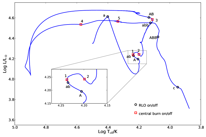
Figure 1: HR diagram of the evolution of the primary star in a system with a primary mass of $15.7\,{\rm M}_{\odot}$, a secondary mass of $12.56\,{\rm M}_{\odot}$ ($q=0.8$), an initial orbital period of $3$ days and a $\beta$ parameter of $0.5$. The start and end of RLOF is indicated with a black circle: case A (on:a, off:A), case AB (on:ab, off: AB), case ABB (on:abb, off:ABB), case C (on:c). The start and end of central nuclear burning is indicated with a red square: central hydrogen burning off (1), central helium burning on (2), off (3) and central carbon burning on (4) and off (5).

We show the evolution of a representative system of this class on the Hertzsprung-Russell diagram in Fig. 1, its mass loss history in Fig. 2 and the evolution of its internal structure on the Kippenhahn diagram in Fig. 3. This particular system has an initial primary mass of $15.7\,{\rm M}_{\odot}$, a secondary mass of $12.56\,{\rm M}_{\odot}$ (corresponding to $q=0.8$), an initial orbital period of $3$ days and is evolved with $\beta=0.5$. The primary reaches its Roche lobe after $0.94\times 10^{7}$ years (see Fig 1, 3) when the helium mass fraction in the core is $0.89$. This initiates mass transfer through RLOF. As seen in Fig. 2, this initially takes place at a fairly high rate (thermal time scale) . This is the so-called rapid Case A mass transfer phase (Pols, 1994; Wellstein et al., 2001), during which the primary loses about $9\,{\rm M}_{\odot}$. After the mass ratio reverses, the mass transfer slows down to values around $\sim 10^{-6}\,{\rm M}_{\odot}$ yr^-1, driven by the nuclear evolution of the star.

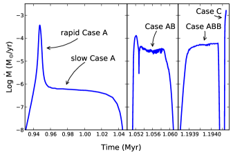
Figure 2: Details of the mass transfer rate as a function of time for Case A system. Three distinct phases are visible. The left panel shows the mass transfer rate during core hydrogen burning. The middle panel shows the mass transfer rates during hydrogen shell burning. The last panel shows mass transfer rates during and after carbon burning, cf. Fig. 3. The rise in mass transfer rate at the very end is a result of instabilities arising in the envelope and will be discussed in Sec. 4.2.

During this phase the star loses another $0.4\,{\rm M}_{\odot}$, and finishes this first mass transfer phase with a total mass of $6.23\,{\rm M}_{\odot}$, and a helium core mass of $1.75\,{\rm M}_{\odot}$. The ignition of the hydrogen burning shell causes the star to expand, which starts the second mass transfer phase, the so-called Case AB phase ( Wellstein et al., 2001), which proceeds on the thermal timescale of the star. During this phase mass transfer rates are of the order of $3\times 10^{-5}\,{\rm M}_{\odot}$ yr^-1, and the star loses an additional $3\,{\rm M}_{\odot}$ so that the total mass left is $3.24\,{\rm M}_{\odot}$ (which, in this system, corresponds to the mass of the convective hydrogen core at the time Case A mass transfer started, see Fig. 3). At this time the helium core measures $2.13\,{\rm M}_{\odot}$, which through subsequent hydrogen shell burning grows to $3.08\,{\rm M}_{\odot}$. Once Case AB mass transfer finishes, , and the star moves to the left side of the Hertzsprung Russell diagram, becoming a hot and compact helium star (see Fig 1). The star finishes helium core burning at $1.172\times 10^{7}$ yr and subsequent core compression ignites helium shell burning By the time that convective carbon burning starts in the core, a CO core of $1.29\,{\rm M}_{\odot}$ has formed. Throughout the carbon burning phase (various carbon flashes), which lasts from $1.192\times 10^{7}$ yr till $1.194\times 10^{7}$ yr (about $20,000$ yrs), the star forms a core composed of neon and oxygen. Another episode of mass transfer starts during the final carbon flashes (the third panel in Fig. 2, also marked in Fig. 3) which erodes the final bit of the remaining hydrogen layer and cancels hydrogen burning.

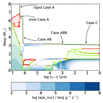
Figure 3: Kippenhahn plot of the donor of our Case A system. The total mass is indicated by the solid black line. The green hatched regions indicates areas of convection, while the red hatched regions indicate semi-convection. Regions of nuclear energy generation are marked with blue shading. Only the inner $8\,{\rm M}_{\odot}$ of the star are shown. As the later phases in the evolution take place on a much shorter timescale, the x-axis is plotted with a logarithmic scale.

By the end of carbon burning the ONe core has a mass of $1.19\,{\rm M}_{\odot}$ while the CO core has a mass of $1.34\,{\rm M}_{\odot}$. During the last carbon shell flash a convective shell forms on top of the helium burning shell, which slowly diminishes the helium burning intensity. This also slows down the growth of the CO core, which is able to grow to a mass of $1.40\,{\rm M}_{\odot}$ by the end of the model run. Significant mass loss develops at the very end of the model run and causes instabilities that terminate the model (see also Section 4.2). During the evolution of the primary, the secondary has grown by $\sim 6\,{\rm M}_{\odot}$ to a total mass of $18.58\,{\rm M}_{\odot}$. Although it is now much more massive than the primary, it is still a main sequence star (hydrogen mass fraction of $0.03$) due to the accretion of large amounts of fresh hydrogen, causing the star to rejuvenate (Hellings, 1983; de Mink et al., 2014; Schneider et al., 2016). If the primary is able explode and forms a neutron star, this system most likely evolves into an Be/X-ray binary.

3.2 Case B Evolution

Stars that undergo their first mass transfer during hydrogen shell burning are considered Case B mass transfer systems. The removal of high-entropy layers of the envelope causes he star to shrink on a dynamical timescale, however, as the donor expands on the thermal timescale during the crossing of the Hertzsprung gap this leads to stable but high mass transfer rates of $\sim 10^{-4}-10^{-3}\,{\rm M}_{\odot}$ yr^-1. Early Case B mass transfer will affect the formation of the helium core as the intensity of hydrogen shell burning is diminished as a result of the envelope responding to the high mass loss rates. Late Case B mass transfer will have less of an effect as the helium core has already been established by the time mass transfer starts. Because the time of the beginning of Case B mass transfer has a strong influence on the subsequent evolution, we discuss three different Case B systems in order to establish a clear picture of Case B evolution.

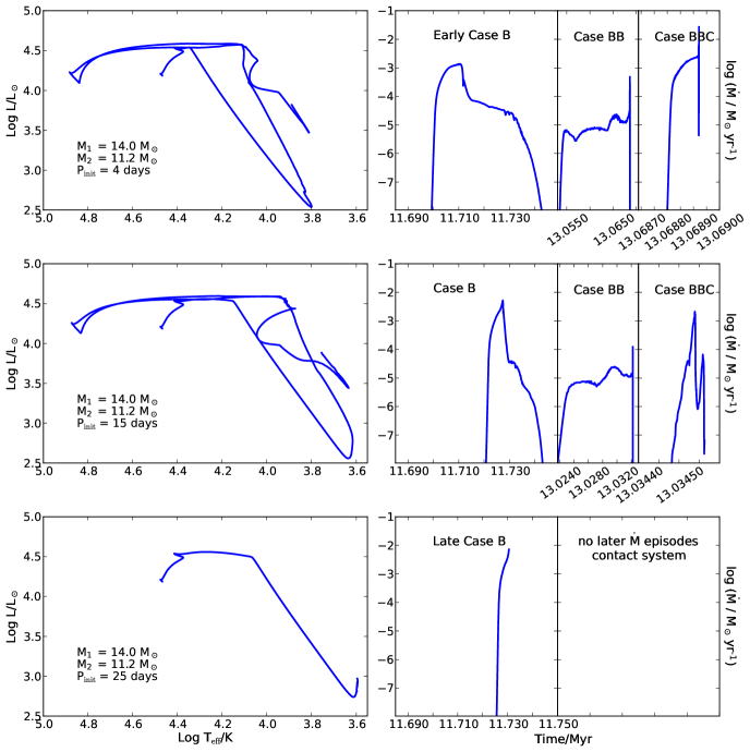
Figure 4: Evolution of a binary system with $M_{1}=14.0\,{\rm M}_{\odot}$ and $M_{2}=11.2\,{\rm M}_{\odot}$, with three different initial orbital periods, corresponding to early Case B mass transfer (4 days, top row), intermediate Case B mass transfer (15 days, middle panel) and late Case B mass transfer (25 days, bottom panel). The left column shows the Hertzsprung-Russell diagram for the three systems, the right column shows the mass transfer history as a function of time for the three systems. While the first window of each mass loss panel has the same scale and allows for comparison between the timing of the onset of mass transfer, later phases are zoomed in considerably to show detail and have different scales on the time axis.

Fig. 4 shows the evolution of three Case B systems (an early, mid, and late Case B system). System 1 (top row), an early Case B system ($M_{1}=14.0\,{\rm M}_{\odot}$, $M_{2}=11.2\,{\rm M}_{\odot}$, $P_{\mathrm{init}}=4$ days), started mass transfer promptly after the primary star finished core hydrogen burning and started crossing the Hertzsprung gap ($t_{\mathrm{RLOF1}}$ = 11.6998 Myr). Mass transfer rates of $\sim 10^{-3}\,{\rm M}_{\odot}$ yr^-1 are seen for approximately $10,000$ yrs during which the primary loses $9.8\,{\rm M}_{\odot}$. After the mass ratio reverses and the orbit widens again as a response to the mass transfer, the star is able to adjust its thermal structure, and around $11.71$ Myr a period of slower mass transfer commences (slow Case B, Paczyński 1971; Doom 1984) with rates of $\sim 3\times 10^{-5}\,{\rm M}_{\odot}$ yr^-1 (Fig 4, top right). The separation of the binary components increases from $31\,{\rm R}_{\odot}$ at the start of Roche lobe overflow to $\sim 100\,{\rm R}_{\odot}$ after the fast Case B phase, and $150\,{\rm R}_{\odot}$ ($48$ days) after the first mass transfer phase finishes (i.e. when helium ignited in the core). the star shrinks in response to this, and experiences a pause in mass transfer. As a result, the star is able to evolve through core helium burning relatively unaffected. After helium core burning the primary has a mass of $3.3\,{\rm M}_{\odot}$, with a helium core of $3.11\,{\rm M}_{\odot}$ and a CO core of $1.29\,{\rm M}_{\odot}$. mass transfer through Roche lobe overflow during the subsequent core carbon burning . for $\sim 20,000$ years at a rate of $\sim 5\times 10^{-5}\,{\rm M}_{\odot}$ yr^-1 during which the star loses its residual hydrogen layer of $0.2\,{\rm M}_{\odot}$. At the end of its evolution the star has established an helium core of $3.{12}\,{\rm M}_{\odot}$, a CO core of $1.{40}\,{\rm M}_{\odot}$ and an ONe core of $1.{35}\,{\rm M}_{\odot}$. The final orbital separation of the system is $\sim 175\,{\rm R}_{\odot}$.

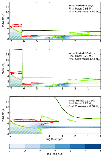
Figure 5: Kippenhahn diagrams for three Case B systems discussed in the text. The total mass is indicated by the solid black line. The green hatched regions indicates areas of convection, while the red hatched regions indicate semi-convection. Regions of nuclear energy generation are marked with blue shading. Time is plotted on the $x$-axis, with the value of $t_{\mathrm{f}}-t$/yr indicating the remaining time in the calculation, plotted logarithmically to show detail in the later phases of the evolution.

System 2 (Fig. 4, middle row) is a binary system ($M_{1}=14.0\,{\rm M}_{\odot}$, $M_{2}=11.2\,{\rm M}_{\odot}$, $P_{\mathrm{init}}=15$ days) that experiences the start of Roche lobe overflow in the middle of the Hertzsprung gap ($t_{\mathrm{RLOF1}}$ = 11.7210 Myr). mass transfer rates quickly increase to values of $\sim 5\times 10^{-3}\,{\rm M}_{\odot}$ yr^-1 during which $10.4\,{\rm M}_{\odot}$ is lost from the primary, leaving a donor with a mass of $3.6\,{\rm M}_{\odot}$, a helium core of $3.18\,{\rm M}_{\odot}$ and a CO core of $1.31\,{\rm M}_{\odot}$ at the completion of core helium burning. Due to adjustments to the thermal structure of the star during the contraction of the CO core, mass loss increases again during the carbon burning phase (Fig. 5, middle row, Case BB, $t_{\mathrm{RLOF2}}$ = 13.0237 Myr), but now at relatively low rates of $\sim 7\times 10^{-5}\,{\rm M}_{\odot}$ yr^-1. This moderate mass loss removed almost the entire residual hydrogen envelope, and leaves a star with mass of ${3.23}\,{\rm M}_{\odot}$, a He core of ${3.22}\,{\rm M}_{\odot}$, a CO core of ${1.42}\,{\rm M}_{\odot}$ and a ONe core of ${1.38}\,{\rm M}_{\odot}$. During the fast Case B mass transfer period, the orbit increased from $75\,{\rm R}_{\odot}$ (initial) to $345\,{\rm R}_{\odot}$, which increases during subsequent mass loss episodes to $370\,{\rm R}_{\odot}$. While the initial period of this system was quite a lot larger than system 1, the evolution of system 2 proceeded very similar to that of system 1. While system 1 starts mass transfer earlier, system 2 reaches higher mass transfer rates due to its higher mass and shorter Kelvin-Helmholz timescale. Both mass loss episodes terminate when helium ignites in the core (roughly about the same time, $t=1.1742\times 10^{7}$ yr, see Fig. 4), and consequently the amount of mass transferred during the first mass transfer phase is about equal ($\sim 10\,{\rm M}_{\odot}$).

System 3 (Fig. 4, bottom row) shows the evolution of a binary system ($M_{1}=14.0\,{\rm M}_{\odot}$, $M_{2}=11.2\,{\rm M}_{\odot}$, $P_{\mathrm{init}}=25$ days) that experiences the start of Roche lobe overflow late in the Hertzsprung gap ($t_{\mathrm{RLOF1}}$ = 11.7250 Myr). As the primary expands beyond its Roche lobe, mass transfer rates quickly ramp up to values of $7.7\times 10^{-3}\,{\rm M}_{\odot}$ yr^-1. Although the orbital separation increases, and thus the size of both Roche lobes, the secondary quickly fills its Roche lobe due to the large amount of accreted matter, leading to a contact system after only $4500$ yrs (cf. de Mink et al., 2008b; Langer, 2012; de Mink et al., 2013).

When evolved with different values of $\beta$, only the $\beta=0.75$ is able to avoid contact, as the lower mass accretion rates and faster growing orbit allow the accretor to respond more efficiently to mass accretion, leading to less swelling and avoiding contact.

4 The Effects of Mass Loss on the Evolution of the Primary

In order to explode as an ECSN several ingredients need to be in place. Nomoto (1984) argued that stars with helium cores between $2.0$ and $2.5\,{\rm M}_{\odot}$ (which corresponds to roughly to initial masses between $8$ and $10\,{\rm M}_{\odot}$) would explode as an ECSN. His models, however, did not develop a second dredge-up which significantly reduce the mass of the helium core and diminishes the predictive power of this criterion (cf. Podsiadlowski et al., 2004; Poelarends et al., 2008). Since then, several authors (Siess, 2007; Poelarends et al., 2008; Jones et al., 2013; Doherty et al., 2010, 2015) have established precise initial mass ranges for ECSN to occur, although these mass ranges are highly sensitive to the adopted convection criteria, overshooting and mass loss prescriptions (Poelarends et al., 2008; Doherty et al., 2010; Langer, 2012). Jones et al. (2013) produced several detailed models, computed all the way to electron captures on ²⁴Mg and ²⁰Ne, and found that CO cores over $1.35\,{\rm M}_{\odot}$ are able to reach densities high enough for this to occur ($\log\rho\approx 9.6$ g cm^-3). If the CO core is massive enough, neon will ignite off center (Jones et al., 2013; Schwab et al., 2016), but Jones et al. (2014) also found that the upper boundary for ECSN is affected by uncertainties regarding the progression or stalling of the neon flame. There seems to be consensus, however, that the mass of the CO core is a reliable indicator for the final fate of stars in this mass range.

The question, however, is whether the range in $M_{\mathrm{CO}}$ for ECSN in binaries is identical to the established $M_{\mathrm{CO}}$ range for ECSN in single stars. Our models indicate that this might not necessarily be the case. Whereas CO cores with a mass of $\sim 1.42\,{\rm M}_{\odot}$ in single stars would ignite neon in their cores (cf. Nomoto, 1984, 1987; Jones et al., 2013) our models do not show neon ignition due to a slightly lower central temperature. This rather different behavior is a direct result of the binary interaction, and thus unique to binary systems. We have identified, and will describe below, two processes that are responsible for that. Compared to single stars, significant mass loss before the establishment of the CO core will create a smaller CO core and lead to a consistently lower temperature . In addition, mass loss during and after carbon burning will cause the star to cool down faster compared to its single star counterpart even if the core mass is the same.

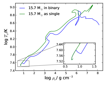
Figure 6: Evolution of the central density versus central temperature. Shown in blue is our Case A model which undergoes mass transfer once the temperature reaches $\log T/K=7.6$. Shown in green is a single star model of the same initial mass ($15.7\,{\rm M}_{\odot}$). the star that undergoes mass transfer develops a core that is cooler and more compact (higher density) compared to a single star of the same initial mass. The single star eventually develops off center neon burning and a CO core with a mass of $1.63\,{\rm M}_{\odot}$, while the star in the binary avoids neon burning and develops a CO core of $1.40\,{\rm M}_{\odot}$.

4.1 Mass Loss During Hydrogen or Helium Burning

Significant mass transfer due to RLOF anytime before the establishment of the CO core will affect the subsequent formation of the CO core. that undergo Case A mass transfer form smaller cores than their single star counterparts.

Case B systems do not show the notable decrease in central temperature upon the start of mass transfer,

The net effect is that CO cores are smaller than those of single stars.

4.2 Mass Loss After Core Carbon Burning

After central carbon burning, in the absence of a heat source, the core contracts again to maintain hydrostatic equilibrium. Due to this contraction at high central densities, neutrino losses increase and degeneracy sets in, resulting in a degenerate core which is governed by the balance between heating due to contraction and cooling due to neutrino losses (Paczyński, 1971; Nomoto, 1984; Brooks et al., 2016). In single stars, helium shell burning would cause the core to grow, and cooling as a result of neutrino losses would be offset by additional heating as a result of accretion due to core growth. However, all of our models experience significant mass transfer (with rates up to, and sometimes exceeding, $\dot{M}>10^{-3}\,{\rm M}_{\odot}$ yr^-1). This pushes the star out of thermal equilibrium, leading to additional cooling in the core as a result of an endothermic expansion to make up for lost envelope matter (an effect similar to what has been found by Tauris et al., 2015; Schwab et al., 2016).

shows the effect of high mass loss rates this late in the evolution of the star on the central temperature.

This difference in minimum $M_{\mathrm{CO}}$ needed for neon ignition between single stars and binary stars is also seen in Fig. 4.2 where we plot the final $M_{\mathrm{CO}}$ against the maximum temperature that a core attained during its evolution. The horizontal dotted line shows the approximate temperature that is necessary for neon to ignite. For simplicity we take a value of $\log T/\mathrm{K}=9.1$, although this might vary slightly depending on the density as the right panel shows. The red crosses represent single star models with initial masses from $12.0-13.0\,{\rm M}_{\odot}$ (spaced by $0.05\,{\rm M}_{\odot}$). These cross the $\epsilon_{\mathrm{Ne}}=\epsilon_{\nu}$ line at $M_{\mathrm{CO}}=1.37\,{\rm M}_{\odot}$, in good agreement with Nomoto (1984); Jones et al. (2013); Takahashi et al. (2013); Schwab et al. (2016). The filled symbols represent several binary model runs. Binary Sequence A consists of stars with initial parameters: $M_{1}=13.8-15.2\,{\rm M}_{\odot}$ (spaced by $0.1\,{\rm M}_{\odot}$), $q=M_{2}/M_{1}=0.8$, and $P_{\mathrm{init}}=15$ days. Binary Sequence B consists of stars with initial parameters: $M_{1}=13.5-15.5\,{\rm M}_{\odot}$ (spaced by $0.1\,{\rm M}_{\odot}$), $q=M_{2}/M_{1}=0.9$, and $P_{\mathrm{init}}=20$ days. Binary Sequence C consists of stars with initial parameters: $M_{1}=13.6-15.2\,{\rm M}_{\odot}$ (spaced by $0.1\,{\rm M}_{\odot}$), $q=M_{2}/M_{1}=0.8$, and $P_{\mathrm{init}}=9$ days. All sequences have a mass transfer efficiency of $\beta=0.5$. only crosses the $\epsilon_{\mathrm{Ne}}=\epsilon_{\nu}$ line at $M_{\mathrm{CO}}=1.52\,{\rm M}_{\odot}$. The conclusion is that stars in binaries, experiencing high RLOF mass transfer rates, need $M_{\mathrm{CO}}>1.52\,{\rm M}_{\odot}$ to be able to develop conditions that will lead to neon ignition. To this effect, the neon ignition boundary shown in Fig. 8 and Fig. 9 is positioned at a $M_{\mathrm{CO}}=1.52\,{\rm M}_{\odot}$, which we take as the boundary between possible ECSN progenitors (lower masses) and CCSN progenitors (higher masses).

5 The Mass Range for ECSN

Based on our results described above, we are now in the position to discuss the parameter space where conditions for ECSN are favorable. A total of approximately 45,000 binary sequences were calculated to investigate the ECSN channel in binary stars. A small fraction of the models (approximately $2000$) suffered numerical instabilities during their evolution and were terminated because of that. These models were ignored in the final analysis. Most models, however, capture the evolution of the stellar models through carbon burning and the formation of an ONe core, unless the system developed contact. The final fate of our models can therefore be characterized by six different outcomes, which are summarized below and shown in Fig. 7 for one particular combination of parameters, i.e. $\beta=0.5$ and $q=0.7$. The full grid is shown in Fig. 8 and will be discussed in more below.

• (Long-P-contact) Binary systems with a long initial period will develop contact as well, due to the high mass transfer rates which prevent the secondary to adjust sufficiently fast enough to avoid filling its Roche lobe (indicated with yellow symbols). The late Case B model described in Sec. 3.2 is part of this class.

• (ONe WD) Models with a low initial primary mass ($\mathrel{\hbox{\hbox to0.0pt{\lower 2.36806pt\hbox{$\sim$}\hss} \kern-3.00003pt\raise 1.72218pt\hbox{$<$}}}13.5\,{\rm M}_{\odot}$) will develop a massive ONe WD (indicated with green symbols).

• (CCSN) Models with a high initial primary mass ($\mathrel{\hbox{\hbox to0.0pt{\lower 2.36806pt\hbox{$\sim$}\hss} \kern-3.00003pt\raise 1.72218pt\hbox{$>$}}}15.2\,{\rm M}_{\odot}$) will develop neon burning and will evolve toward a CCSN (indicated with red symbols).

• (Case B ECSN) Models with a period between $\sim{4}$ days and an upper bound that depends on the values of $\beta$ and $q$ and initial primary masses of $\sim 13.5-15.2\,{\rm M}_{\odot}$ develop Case B mass transfer and a CO core that falls with a mass between $1.37\,{\rm M}_{\odot}$ and $1.52\,{\rm M}_{\odot}$ (indicated with blue symbols, ECSN - Case B).

• (Case A ECSN) Models with an initial period that is between $\sim{2.5}$ days will develop late Case A mass transfer. primary initial mass range shifts with respect to Case B systems(indicated with blue symbols, ESCN - Case A).

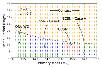
Figure 7: Expected final fate of computed models in our grid for $\beta=0.5$ and $q=0.8$ as a function of initial primary mass and initial period. Five distinct outcomes are visible and labeled. ECSN are indicated by blue dots.

In Fig. 7 we show these final evolutionary outcomes for a particular combination of parameters, i.e. $\beta=0.5$ and $q=0.7$ (compare also with Wellstein et al. 2001, Fig. 12). ECSN progenitors have a minimum mass of $13.7\,{\rm M}_{\odot}$ which increases to $13.9\,{\rm M}_{\odot}$ for early Case B systems (analogical to the much larger shift in initial mass for Case A systems). The upper mass limit for ECSN progenitors is found at $15.1\,{\rm M}_{\odot}$ with a slight shift to higher initial masses ($15.3\,{\rm M}_{\odot}$) for early Case B systems. This boundary forms the transition to progenitors that develop neon burning. Case A ECSN progenitors can be found at $P_{\mathrm{init}}=3$ days, between $M_{1}=15.7\,{\rm M}_{\odot}$ and $M_{1}=16.4\,{\rm M}_{\odot}$. For this particular combination of $q$ and $\beta$, the minimum period for systems to develop contact decreases from about $20$ days at $M_{1}=13.5\,{\rm M}_{\odot}$ to $\sim 10$ days at $M_{1}=16.5\,{\rm M}_{\odot}$. This limits the number of ECSN candidates at higher initial masses, but also the progenitors that develop neon burning.

As can be seen, most combinations of $q$ and $\beta$ behave qualitatively similar, although the boundaries between contact systems and non-contact systems shift for various combinations of $q$ and $\beta$.

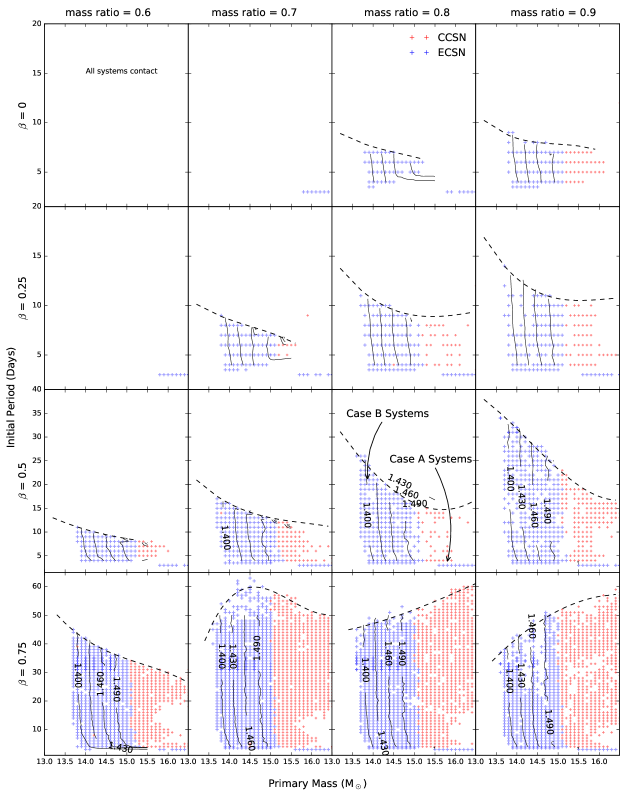
Figure 8: ECSN (blue) and CCSN models (red) as a function of initial primary mass and initial period, for $\beta=0,0.25,0.5,0.75$ and mass ratios $q=0.6,0.7,0.8,0.9$.The initial period for the two top rows is limited to $20$ days, and the third row to $40$ days as systems with larger periods evolve all to contact binaries. Case A and Case B systems are indicated in the panel for ($q$,$\beta$) = (0.8, 0.5) and are representative for all other panels. Masses of the pre-ECSN CO cores are indicated with contour lines, marking the location of $1.40,1.43,1.46$, and $1.49\,{\rm M}_{\odot}$. The approximate boundary between contact and contact-free systems is indicated by a dashed line.

the initial primary mass for ECSN is confined to a narrow range between $13.6\,{\rm M}_{\odot}$ and $15.1\,{\rm M}_{\odot}$ for Case B systems and between $15.5\,{\rm M}_{\odot}$ and $17.6\,{\rm M}_{\odot}$ for Case A. For fully conservative evolution ($\beta=0$) the initial periods for systems Case B mass transfer that result in an ECSN are confined to $P_{\mathrm{init}}<10$ days and mass ratios $q>0.75$. Several Case A systems are found for initial primary masses between $15.8\,{\rm M}_{\odot}$ and $16.4\,{\rm M}_{\odot}$ at a period of $3.5$ days. All Case B systems for mass ratios below $0.7$ , however, there are Case A systems with an initial period of $3$ days and initial primary masses between $15.8\,{\rm M}_{\odot}$ and $16.3\,{\rm M}_{\odot}$.

For non-conservative evolution the mass range for ECSN barely changes, however, the range in initial periods does increase. For $\beta=0.25$ (25% of the mass lost from the primary star is expelled from the system) the maximum period increases to about $\sim 15$ days for a mass ratio near unity and decreases to $10$ days for a mass ratio of $0.70$.

For non-conservative evolution with $\beta=0.5$ ($50$% accreted, $50$% expelled) the maximum initial period for Case B systems increases to $33$ days for $q=0.9$, to $25$ days for $q=0.8$ and to $17$ days for $q=0.7$. The systems discussed in Section 3 are part of this data set. Case A mass transfer leading to ECSN occurs for all mass ratios, while Case B mass transfer is still limited to $0.7<q<1$.

The situation for the non-conservative case with $\beta=0.75$ ($75$% expelled, $25$% accreted) is a bit different as the maximum period for ECSN formation increases from $50$ days in the $q=0.9$ case to $57$ days in the $q=0.7$ case. Models with a value of $\beta=0.75$ form the only instance for $q=0.6$ that shows ample evidence for Case B systems able to evolve to a ECSN. These Case B systems are found between $13.7\,{\rm M}_{\odot}$ and $15.0\,{\rm M}_{\odot}$ with an initial period between $4$ days and $45$ days.

6 Discussion and Conclusions

We have presented close binary systems where the primary star could potentially be the progenitor of an ECSN. While the mass range for ECSN in single stars is fairly narrow (Poelarends et al., 2008), the mass range for ECSN in binary stars is thought to be much wider as the effects of mass loss due to Roche lobe overflow are thought to mitigate the effects of the second dredge-up in single stars (Podsiadlowski et al., 2004). this second dredge-up reduces the mass of the helium core below the Chandrasekhar mass (in the relevant initial mass range) and makes that the possibility for an ECSN depends on the outcome of the race between core-growth and envelope mass loss during the SAGB (Poelarends et al., 2008; Takahashi et al., 2013). If the core is able to contract to high enough densities so that electron captures on ²⁴Mg and ²⁰Ne can commence, heating as a result of these electron captures will cause O+Ne burning at the center, and O+Ne deflagration propagates outward. Core contraction is further accelerated by electron captures in the central nuclear statistical equilibrium region, resulting in a weak Type II supernova (Takahashi et al., 2013; Kitaura et al., 2006). However, if mass loss removes the envelope fast enough so that the core is not able to reach those critical densities, the star will evolve into a massive ONe white dwarf.

Our study, however, has focused on binary systems instead of single stars and attempts to answer two major questions concerning: First, are binary systems indeed capable of producing and ECSN, and, second, what is the expected region in the ($M_{1}$, $M_{2}$, $P_{\mathrm{init}}$) phase space that we can expect these ECSN to occur? We have investigated these questions by running approximately 45,000 binary models in the relevant phase space.

6.1 The Possibility of ECSN from Close Binary Systems

Based on single star models there is consensus in the literature that a star will experience an ECSN when $M_{\mathrm{CO}}$ is somewhere between $\sim 1.37$ and $\sim 1.42\,{\rm M}_{\odot}$ (see for example Woosley & Heger, 2015; Tauris et al., 2015; Moriya & Eldridge, 2016, who all adopt similar values). Tauris et al. (2015) , in the context of ultra-stripped supernovae, use as a “rule of thumb” (based on single star models) that the upper boundary is given by stars that develop a post-carbon burning central temperature above their carbon burning central temperature as these conditions will lead to an iron core collapse. In this case the ignition of neon and oxygen burning will eventually convert the composition of the entire core into ²⁸Si and ³²S, bringing the chance for contraction due to electron captures to an end. Their lower boundary is given by the ONe WD threshold of $1.37\,{\rm M}_{\odot}$, as these cores are not able to contract to sufficiently high densities where electron captures can commence.

Based on the models presented above, however, we question whether these boundaries can be applied to stars in a binary system, as mass loss driven by Roche lobe overflow, especially after central carbon burning drives the star out of thermal equilibrium, leading to significant expansion and a much stronger cooling in the core than in single stars. While in single stars the effect of neutrino cooling is compensated by heating due to core growth, keeping the central temperature of the star roughly constant during the post-carbon burning contraction (Nomoto, 1984), in binary stars the cooling is enhanced by mass loss. Nevertheless, many ingredients for this contraction are different from the evolution of single stars, and a simple comparison of evolutionary tracks in the $\rho_{\mathrm{c}}-T_{\mathrm{c}}$ plane is not possible. This scenario would apply to all cores that do not ignite neon ($M_{\mathrm{core}}\lesssim 1.52\,{\rm M}_{\odot}$) down to the effective Chandrasekhar mass ($\sim 1.40\,{\rm M}_{\odot}$) or possibly even $\sim 1.37\,{\rm M}_{\odot}$ and deserves further investigation.

In case the primary star Once the secondary leaves the main sequence, its expansion will give rise to reverse Roche lobe overflow (De Donder & Vanbeveren, 2003; Zapartas et al., 2017). This will likely happen not immediately, as the binary separation has grown to $\sim 1000\,{\rm R}_{\odot}$. Eventually, however, mass accretion onto the ONe white dwarf will heat up the cold white dwarf, allow core growth to resume, reheat the core and possibly give rise to conditions that are conducive for electron captures to accelerate the heating process. result in the collapse of the core and the formation of a neutron star (Nomoto, 1984; Dessart et al., 2006; Schwab et al., 2016).

6.2 Comparison with Previous Work

The results presented in this paper differ significantly from earlier studies that evaluated the existence of ECSN in binary systems. The first paper to discuss such supernovae in binaries was Podsiadlowski et al. (2004) who concluded that, based on models by Wellstein et al. (2001), initial primary masses between $8\,{\rm M}_{\odot}$ and $17\,{\rm M}_{\odot}$ would be expected to evolve into an ECSN. This estimate was based on the helium core criterion developed by Nomoto (1984) who showed that helium cores between $2\,{\rm M}_{\odot}$ and $2.5\,{\rm M}_{\odot}$ lead to conditions where electron captures will kick off the collapse of the core.

Despite the differences, many of the fundamental ideas in Podsiadlowski et al. (2004) are confirmed by this paper. While their inference was based on only a handful of models that established the relationship between the initial mass and final helium mass of stars in close binary systems, our detailed grid confirms indeed that the spread in $M_{\mathrm{CO}}$ is fundamentally a result of the period, and that the difference in timing of Roche lobe overflow between Case A and Case B systems will result in Case A systems developing smaller cores, effectively shifting their initial mass-final core mass relationship toward higher initial masses.

Our research, however, provides several improvements on Podsiadlowski et al. (2004). First of all, the helium core criterion, developed by Nomoto (1984) might work well for single stars, it, however, gives less accurate results for binary stars. The main reason for this is that close binary systems suffer from significant mass loss , either during the main sequence or in the Hertzsprung gap, which considerably affects the development and mass of the helium core. Although the CO core is not directly affect (i.e. eroded) by mass transfer due to RLOF, there is still an appreciable difference between the evolution of CO cores of the same mass in single stars and in binary systems, as Fig. 4.2 shows. Secondly, whereas Podsiadlowski et al. (2004) expected that mass loss due to Roche lobe overflow would prevent the second dredge-up from happening, we find that mass loss actually has a very similar effect in reducing the mass of the helium core. Indeed, the second dredge-up was avoided, but the mass of the hydrogen envelope and sometimes the underlying helium layer was significantly reduced. Evidence for this erosion of the helium layer was already present in Wellstein et al. (2001), however, it was not considered in Podsiadlowski et al. (2004). Third, our models show that the role of mass loss in the final evolution toward electron captures is much larger than was previously thought. Cores undergoing significant mass loss compensate for this by expansion and enhanced cooling. This leads to massive ONe cores (up to $\sim 1.52\,{\rm M}_{\odot}$) that are able to avoid neon ignition. If the ONe core is able to contract to high enough densities to cause the conditions for electron captures to occur we expect a maximum mass range for Case B systems that is $\sim 2\,{\rm M}_{\odot}$ wide and a maximum mass range for Case A systems that is $\sim 3\,{\rm M}_{\odot}$ wide. When we combine both mass ranges, the maximum mass range for ECSN from binary systems runs from an initial primary mass of $\sim 13.5\,{\rm M}_{\odot}$ to $\sim 18\,{\rm M}_{\odot}$, a width of $\sim 4.5\,{\rm M}_{\odot}$, which is significantly narrower than the prediction of Podsiadlowski et al. (2004) but much wider than the initial mass range for single stars (roughly $0.25\,{\rm M}_{\odot}$, Poelarends et al. 2008). The use of a different convection criterion (e.g. Schwarzschild instead of Ledoux, more efficient semi-convection, or additional convective boundary mixing), will translate the mass range to lower values (possibly somewhere around $\sim 10-15\,{\rm M}_{\odot}$), without affecting the primary conclusions of this paper (c.f., Appendix A, Doherty et al. 2010). This will be further explored in a future publication. Even so, the improvements of the models that we have presented there provide a picture that makes the possibility for ECSN from close binary systems much less likely than originally thought.

Our models are in broad agreement with the results of Tauris et al. (2013, 2015). While their research is focused on helium cores orbiting a compact object, the general evolutionary picture shows lots of similarities (compare Fig. 18 in Tauris et al. 2015 with our Fig. 8). As it is not clear which role mass loss plays in their models, especially during and after carbon burning, we don’t know whether our results are applicable to their situation. Regardless, more research is needed to accurately describe the evolution of massive ONe cores at high densities, whether they converge onto a common evolutionary track in the $\rho_{\mathrm{c}}-T_{\mathrm{c}}$ plane and are able to contract to sufficiently high densities for electron captures to destabilize the core, or that they continue to cool down and avoid electron captures all together. Much of this will determine the exact mass range of ECSN in binary systems as neither the mass of the CO core, nor the track in the $\rho_{\mathrm{c}}-T_{\mathrm{c}}$ plane, are, according to our models, sufficient to uniquely determine the final fate of these stars.

6.3 The Expected Initial Mass Range for ECSN in Close Binary Systems

If we assume that continued core contraction after mass loss ceases will eventually converge the evolution a core onto a common evolutionary track in the $\rho_{\mathrm{c}}-T_{\mathrm{c}}$ plane toward electron captures, we are able to characterize, within the limits of our assumptions on the treatment of convection, overshooting, mixing, and accretion, the initial mass range for ECSN. Figure 9 provides a different way of looking at our dataset, showing the final $M_{\mathrm{CO}}$ as a function of the initial primary mass. The horizontal dashed red at $1.52\,{\rm M}_{\odot}$ indicates the maximum $M_{\mathrm{CO}}$ that avoids neon ignition, and hence forms the upper boundary of the ECSN range. This upper boundary could be shifted to even higher $M_{\mathrm{CO}}$ if neon flames are able to stall (Jones et al., 2014), leaving the chemical composition in the center unaltered and allowing for subsequent electron captures to occur. Most work on stalling flames has been done in the context of carbon flames by Denissenkov et al. (2013, 2015); Farmer et al. (2015) whose research suggest that efficient convective boundary mixing can disrupt inwardly propagating carbon flames, however Lecoanet et al. (2016) find that hybrid cores are unlikely. We defer to future work the investigation of quenched neon flames which might influence our upper boundary for $M_{\mathrm{CO}}$ leading to ECSN. The horizontal dash-dotted green line at $1.4\,{\rm M}_{\odot}$ indicates the Chandrasekhar mass for a composition of 50% neon and 50% oxygen. The horizontal dashed red line at $1.37\,{\rm M}_{\odot}$ indicates the lowest possible CO core mass that is able to evolve into an ECSN.

Two distinct sequences are visible in each panel (cf. Wellstein & Langer, 1999, Fig 5b), Case B models (on the left) and Case A models (on the right). The reason that Case B and Case A systems are separate is that mass loss during the main sequence reduces the hydrogen burning core, effectively shifting the ECSN range to higher initial masses. The scatter in the vertical direction can be attributed to a spread in initial period, with models toward the lower end of the sequence originating from low period binaries, while models toward the higher end of the sequence originating from higher period binaries, giving rise to smaller, resp. larger CO cores (c.f. the discussion in Section 3, see also Wellstein et al. 2001). As argued in Sec. 5, initial periods that are longer than our ECSN candidates lead to contact systems. Thus it appears that for a given initial primary mass the initial period will allow for a certain spread in final $M_{\mathrm{CO}}$. However, the key factor that determines the location of the ECSN channel is the initial primary mass. While the number of models that are able to produce CO cores that are favorable for the development ECSN increases with increasing $\beta$ the ECSN mass range itself does not really shift. This is true for both the Case A ECSN channel as for the Case B ECSN channel. If we allow all cores with $1.37\,{\rm M}_{\odot}\leq M_{\mathrm{CO}}\leq 1.52\,{\rm M}_{\odot}$ to eventually explode as an ECSN we find an initial mass range for ECSN between $13.5\,{\rm M}_{\odot}$ and $15.25\,{\rm M}_{\odot}$ for Case B systems and between $15.4\,{\rm M}_{\odot}$ and $17.6\,{\rm M}_{\odot}$ for Case A systems. This mass range is indicated in Figure 9 with arrows marked “Case B – max” and “Case A – max”, respectively. If we confine the cores that are able to evolve into an ECSN to $M_{\mathrm{CO}}$ between the Chandrasekhar mass ($1.40\,{\rm M}_{\odot}$) and $1.52\,{\rm M}_{\odot}$ the initial mass range for ECSN narrows to $14.2\,{\rm M}_{\odot}$ and $15.25\,{\rm M}_{\odot}$ for Case B systems and between $16.1\,{\rm M}_{\odot}$ and $17.6\,{\rm M}_{\odot}$ for Case A systems. This mass range is indicated in Figure 9 with arrows marked “Case B – min” and “Case A – min”, respectively. As our input physics in terms of convective mixing is similar to Wellstein et al. (2001), i.e. we don’t take into account additional mixing such as convective overshooting or exponentially decreasing diffusion Herwig (2000), we expect that this initial mass range might shift to lower initial masses by $2-3\,{\rm M}_{\odot}$ if additional mixing is taken into account. It should, however, not have significant effects on the evolution or the structure of the models or any of our further conclusions (see App. A).

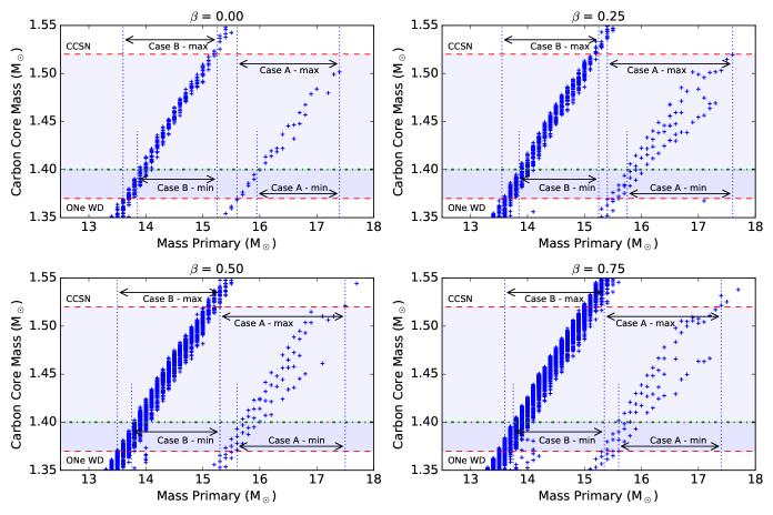
Figure 9: Final $M_{\mathrm{CO}}$ as a function of initial mass, organized by mass transfer efficiency ($\beta$) in four panels. The horizontal dashed red at $1.52\,{\rm M}_{\odot}$ indicates the maximum possible $M_{\mathrm{CO}}$ that does not lead to off-center neon ignition, and thus forms the upper boundary of the ECSN range. The horizontal dash-dotted green line at $1.4\,{\rm M}_{\odot}$ indicates the effective Chandrasekhar mass. The horizontal dashed red line at $1.37\,{\rm M}_{\odot}$ indicates the lowest possible CO core mass that might be able to evolve into an ECSN. The light shaded area between $1.37\,{\rm M}_{\odot}\leq M_{\mathrm{CO}}\leq 1.52\,{\rm M}_{\odot}$ and $1.4\,{\rm M}_{\odot}\leq M_{\mathrm{CO}}\leq 1.52\,{\rm M}_{\odot}$ indicates the maximum and most feasible ECSN range, as long as the decrease in temperature is stopped and the density is able to increase again.

It is worth noting that more ECSN are predicted for systems with a mass ratio close to unity, as the development of contact happens at longer period for higher $q$ systems (see Fig. 8). As the primary star starts transferring mass to the secondary, the orbit shrinks, until the mass ratio is reversed. This reversal happens earlier for mass ratios close to one, and later for lower mass ratios, increasing the chance for contact (de Mink et al., 2013). This primarily affects the numbers of ECSN, not so much the initial mass range (except for Case A systems). This is also true for the value of $\beta$, which controls the amount of matter that is lost from the system (i.e., $\beta=0$ is conservative mass transfer, no mass that is transferred from the primary to the secondary is lost from the system; $\beta=1$ is completely non-conservative mass transfer, all mass that is transferred from the primary is lost from the system, no accretion onto the secondary). For the sake of our parameter study we chose various fixed values of $\beta$, while the mass transfer efficiency in real systems will depend on the evolutionary phase of both stars, the amount of matter already accreted onto the secondary and how that has affected its spinrate. Several mechanisms have been suggested which control the efficiency of mass transfer, mass accretion and mass loss, including the existence of an accretion disk that regulates the amount of mass and angular momentum that can be accreted (Paczyński, 1991; Popham & Narayan, 1991; Deschamps et al., 2013), the necessity of the secondary to stay below critical rotation (Packet, 1981), and the effects of tides on the stellar spins and the stellar orbit (Zahn, 1977; Hurley et al., 2002). Work by Deschamps et al. (2013); van Rensbergen et al. (2008) for systems with slightly lower masses suggests periods with values of $\beta$ close to $1$ (i.e. very inefficient mass transfer), while simulations with a strong tidal interaction (i.e. a short spin-orbit synchronization timescale) suggest shorter periods of moderately inefficient mass transfer (Paxton et al., 2015). Although our models suggest that the efficiency of mass transfer does not really affect the mass range for ECSN, it does, however, strongly affect the range of initial periods that can lead to an ECSN. In addition, the evolution of the secondary will be affected. It will most likely rapidly spin up after the onset of mass transfer and maintain near-critical rotation for possibly extended periods of time. This will induce strong rotational mixing (Langer, 2012; de Mink et al., 2008a, 2013), causing possibly quasi-chemically homogeneous evolution (Maeder, 1987; Langer, 2012) and alter the evolution of the star beyond just the simple fact of mass accretion (Hirschi et al., 2004; de Mink & Mandel, 2016; Marchant et al., 2016). Although it is not clear to what extent this will affect the incidence of ECSN, the effects of tides, mass and angular momentum transfer and loss, and near-critical rotation of the secondary are possibly important and will be discussed in a forthcoming paper, in addition to the effects of additional mixing and convection criteria.

If the scenario turns out to correct, the binary ECSN channel might contribute to the population of NS+NS systems that can be observed with aLIGO/Virgo (Côté et al., 2017). Precursors to these NS+NS systems will be visible as Be/X-ray binaries (Knigge et al., 2011; Shao & Li, 2014).

Appendix A Overshooting, Fast Semi-Convection and the Critical $M_{\mathrm{CO}}$ for Neon Ignition

The models presented in this paper use the Ledoux criterion for determining convective boundaries, and a small amount of semi-convection, $\alpha_{\mathrm{sm}}=0.01$. In order to investigate the robustness of our results against differences in the treatment of convection, we calculated two sequences (similar to the ones presented in Sec. 4.2), one with a stronger semi-convection ($\alpha_{\mathrm{sm}}=1.0$) and the other using overshooting ($f_{\mathrm{ov}}=0.016$, in the context of the Schwarzschild criterion). In this way we are able to determine whether the critical mass for neon ignition (in this paper found to be $M_{\mathrm{CO}}\approx 1.52\,{\rm M}_{\odot}$) shifts to higher or lower $M_{\mathrm{CO}}$ with different convection criteria.

Figure 10 shows these various sequences (including Binary Sequence A from Fig. 4.2), calculated with different treatments of convection. Each sequence was calculated with initial masses between $10.0\,{\rm M}_{\odot}$ and $15.5\,{\rm M}_{\odot}$, for a mass ratio of $q=0.8$, a period of $10$ days and a mass transfer efficiency, $\beta=0.5$. The sequence with $\alpha_{\mathrm{sm}}=1.0$ is shown with yellow symbols, and the sequence with Schwarzschild with $f_{\mathrm{ov}}=0.016$ with blue symbols.

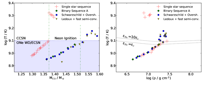
Figure 10: Maximum temperature attained in the core as a function of $M_{\mathrm{CO}}$ (left panel) and as a function of the density at the mass coordinate of $T_{\mathrm{max}}$ at the time of $T_{\mathrm{max}}$ (right panel), for single stars (red crosses) and primary stars in a binary system (filled symbols) with various treatments of convection and overshooting. The dotted line in the left panel approximates the critical temperature for neon ignition, while the dotted lines in the right panel give the locations where the energy generation of neon burning is equal to, and 10 times exceeds the energy losses due to thermal neutrinos.

While we defer a full investigation to a future work, this initial investigation shows that each of these modifications results in a relationship between $M_{\mathrm{CO}}$ and $\log\ T_{\mathrm{max}}$ that is similar to the one shown in Fig. 4.2. This confirms that the critical mass for neon ignition in binary stars is not dependent on the adopted convection criterion, the efficiency of semi-convection, or the use of overshooting. However, each of these different modification does affect the initial mass range by shifting it to lower initial masses (c.f. Poelarends et al. 2008; Doherty et al. 2010).

Appendix B The Effects of Variation of the Spatial and Temporal Resolution

As stellar models can potentially be quite sensitive to the spatial and temporal resolution, we conduct a small-grid resolution study to investigate the robustness of our models against spatial and temporal variations in resolution. While MESA has many parameters that control the temporal and spatial resolution in detail, the parameter $w_{\mathrm{t}}$ controls the overall temporal resolution, and the parameter $\delta_{\mathrm{mesh}}$ controls the overall spatial resolution. The calculations described in this paper were computed with our baseline parameters $w_{\mathrm{t}}=9\times 10^{-4}$ and $\delta_{\mathrm{mesh}}=0.8$. To investigate convergence of our models at a different resolution, we computed a sequence with $w_{\mathrm{t}}=9\times 10^{-4}$ and $\delta_{\mathrm{mesh}}=0.3$ (increased spatial resolution), $w_{\mathrm{t}}=3\times 10^{-4}$ and $\delta_{\mathrm{mesh}}=0.8$ (increased temporal resolution) and $w_{\mathrm{t}}=3\times 10^{-4}$ and $\delta_{\mathrm{mesh}}=0.3$ (increased spatial and temporal resolution). The results are plotted in Fig. 11. The left panel shows the initial mass of the star versus the final $M_{\mathrm{CO}}$, comparable to Fig. 9. The models with the baseline values are shown as green diamonds, while the variations in $w_{\mathrm{t}}$ and $\delta_{\mathrm{mesh}}$ are shown with plus signs. A minimal spread can be seen in the resulting $M_{\mathrm{CO}}$, with models with $w_{\mathrm{t}}=9\times 10^{-4}$ slightly more massive than models with $w_{\mathrm{t}}=3\times 10^{-4}$. The middle panel shows the maximum temperature attained in the core, plotted against the CO core mass (similar to Fig. 4.2). This panel shows excellent model convergence in the mass range considered, with no impact due to changes in spatial or temporal resolution. The location of $T_{\mathrm{max}}$ (shown in the far right panel) is a bit more sensitive to changes in the spatial and temporal resolution, but this can also be attributed to a steep relationship between $M_{\mathrm{CO}}$ and $M_{\mathrm{Tmax}}$ (c.f. Fig. C2 in Schwab et al. 2016). However, this variation has no impact on any of our results.

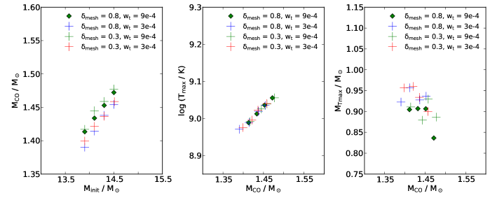
Figure 11: Results of our resolution study. Our baseline parameters are shown as green diamonds while variations in $w_{\mathrm{t}}$ and/or $\delta_{\mathrm{mesh}}$ are shown with colored plus signs. The left panel shows the initial primary mass versus final CO core mass. The middle panel shows the CO core mass versus $T_{\mathrm{max}}$, and the right panel shows the CO core mass versus the radial mass coordinate of $T_{\mathrm{max}}$. All panel shows that our baseline models are within the convergence envelope and thus producing reliable results.

Based on this resolution study we conclude that our baseline parameters lead to good model convergence, and are comparable to models with a higher spatial and/or temporal resolution. The most notable difference is that our baseline models produce more massive cores than models with a higher spatial and temporal resolution. While this does not affect the relationship between the maximum temperature attained in the core and the CO core mass, a higher resolution grid would shift the initial mass range to higher initial primary masses.

References

- Abbott et al. (2016) Abbott, B. P., Abbott, R., Abbott, T. D., Abernathy, M. R., Acernese, F., Ackley, K., Adams, C., Adams, T., Addesso, P., Adhikari, R. X., & et al. 2016, Living Reviews in Relativity, 19, 1
- Almeida et al. (2017) Almeida, L. A., Sana, H., Taylor, W., Barbá, R. ., Bonanos, A. Z., Crowther, P., Damineli, A., de Koter, A. ., de Mink, S. E., Evans, C. J., Gieles, M., Grin, N. J. a nd Hénault-Brunet, V., Langer, N., Lennon, D., Lockwood, S., Maíz Apellániz, J., Moffat, A. F. J. ., Neijssel, C., Norman, C., Ramírez-Agudelo, O. H., Richardson, N. D., Schootemeijer, A., Shenar, T., Soszyński, I., Tramper, F., & Vink, J. S. 2017, A&A, 598, A84
- Beniamini & Piran (2016) Beniamini, P. & Piran, T. 2016, MNRAS, 456, 4089
- Böhm-Vitense (1958) Böhm-Vitense, E. 1958, ZAp, 46, 108
- Brooks et al. (2016) Brooks, J., Bildsten, L., Schwab, J., & Paxton, B. 2016, ApJ, 821, 28
- Côté et al. (2017) Côté, B., Belczynski, K., Fryer, C. L., Ritter, C., Paul, A., Wehmeyer, B., & O’Shea, B. W. 2017, ApJ, 836, 230
- Das & Mukhopadhyay (2013) Das, U. & Mukhopadhyay, B. 2013, Physical Review Letters, 110, 071102
- De Donder & Vanbeveren (2003) De Donder, E. & Vanbeveren, D. 2003, New A, 8, 415
- de Mink et al. (2008a) de Mink, S. E., Cantiello, M., Langer, N., Yoon, S.-C., Brott, I., Glebbeek, E., Verkoulen, M., & Pols, O. R. 2008a, in IAU Symposium, Vol. 252, The Art of Modeling Stars in the 21st Century, ed. L. Deng & K. L. Chan, 365–370
- de Mink et al. (2013) de Mink, S. E., Langer, N., Izzard, R. G., Sana, H., & de Koter, A. 2013, ApJ, 764, 166
- de Mink & Mandel (2016) de Mink, S. E. & Mandel, I. 2016, MNRAS, 460, 3545
- de Mink et al. (2007) de Mink, S. E., Pols, O. R., & Hilditch, R. W. 2007, A&A, 467, 1181
- de Mink et al. (2008b) de Mink, S. E., Pols, O. R., & Yoon, S.-C. 2008b, in American Institute of Physics Conference Series, Vol. 990, First Stars III, ed. B. W. O’Shea & A. Heger, 230–232
- de Mink et al. (2014) de Mink, S. E., Sana, H., Langer, N., Izzard, R. G. ., & Schneider, F. R. N. 2014, ApJ, 782, 7
- Denissenkov et al. (2013) Denissenkov, P. A., Herwig, F., Truran, J. W., & Paxton, B. 2013, ApJ, 772, 37
- Denissenkov et al. (2015) Denissenkov, P. A., Truran, J. W., Herwig, F., Jones, S., Paxton, B., Nomoto, K., Suzuki, T., & Toki, H. 2015, MNRAS, 447, 2696
- Deschamps et al. (2013) Deschamps, R., Siess, L., Davis, P. J., & Jorissen, A. 2013, A&A, 557, A40
- Dessart et al. (2006) Dessart, L., Burrows, A., Ott, C. D., Livne, E., Yoon, S.-C., & Langer, N. 2006, ApJ, 644, 1063
- Doherty et al. (2014a) Doherty, C. L., Gil-Pons, P., Lau, H. H. B., Lattanzio, J. C., & Siess, L. 2014a, MNRAS, 437, 195
- Doherty et al. (2014b) Doherty, C. L., Gil-Pons, P., Lau, H. H. B., Lattanzio, J. C., Siess, L., & Campbell, S. W. 2014b, MNRAS, 441, 582
- Doherty et al. (2015) Doherty, C. L., Gil-Pons, P., Siess, L., Lattanzio, J. C., & Lau, H. H. B. 2015, MNRAS, 446, 2599
- Doherty et al. (2010) Doherty, C. L., Siess, L., Lattanzio, J. C., & Gil-Pons, P. 2010, MNRAS, 401, 1453
- Doom (1984) Doom, C. 1984, A&A, 138, 101
- Duchêne & Kraus (2013) Duchêne, G. & Kraus, A. 2013, ARA&A, 51, 269
- Farmer (2017) Farmer, R. 2017, rjfarmer/pyMesa v1.0.0, zenodo, doi:10.5281/zenodo.846305
- Farmer et al. (2015) Farmer, R., Fields, C. E., & Timmes, F. X. 2015, ApJ, 807, 184
- Garcia-Berro & Iben (1994) Garcia-Berro, E. & Iben, I. 1994, ApJ, 434, 306
- Garcia-Berro et al. (1997) Garcia-Berro, E., Ritossa, C., & Iben, I. J. 1997, ApJ, 485, 765
- Grevesse & Noels (1993) Grevesse, N. & Noels, A. 1993, Physica Scripta, 1993, 133
- Grevesse & Sauval (1998) Grevesse, N. & Sauval, A. J. 1998, Space Sci. Rev., 85, 161
- Heger et al. (2003) Heger, A., Fryer, C. L., Woosley, S. E., Langer, N., & Hartmann, D. H. 2003, ApJ, 591, 288
- Heger et al. (1997) Heger, A., Jeannin, L., Langer, N., & Baraffe, I. 1997, A&A, 327, 224
- Heger et al. (2000) Heger, A., Langer, N., & Woosley, S. E. 2000, ApJ, 528, 368
- Hellings (1983) Hellings, P. 1983, Ap&SS, 96, 37
- Herwig (2000) Herwig, F. 2000, A&A, 360, 952
- Hicken et al. (2007) Hicken, M., Garnavich, P. M., Prieto, J. L., Blondin, S., DePoy, D. L., Kirshner, R. P., & Parrent, J. 2007, ApJ, 669, L17
- Hirschi et al. (2004) Hirschi, R., Meynet, G., & Maeder, A. 2004, A&A, 425, 649
- Hurley et al. (2002) Hurley, J. R., Tout, C. A., & Pols, O. R. 2002, MNRAS, 329, 897
- Iben et al. (1997) Iben, I. J., Ritossa, C., & Garcia-Berro, E. 1997, ApJ, 489, 772
- Itoh et al. (1996) Itoh, N., Hayashi, H., Nishikawa, A., & Kohyama, Y. 1996, ApJS, 102, 411
- Janka (2017) Janka, H.-T. 2017, ApJ, 837, 84
- Janka et al. (2012) Janka, H.-T., Hanke, F., Hüdepohl, L., Marek, A., Müller, B., & Obergaulinger, M. 2012, Progress of Theoretical and Experimental Physics, 2012, 01A309
- Jones et al. (2014) Jones, S., Hirschi, R., & Nomoto, K. 2014, ApJ, 797, 83
- Jones et al. (2013) Jones, S., Hirschi, R., Nomoto, K., Fischer, T., Timmes, F. X., Herwig, F., Paxton, B., Toki, H., Suzuki, T., Martínez-Pinedo, G., Lam, Y. H., & Bertolli, M. G. 2013, ApJ, 772, 150
- Kitaura et al. (2006) Kitaura, F. S., Janka, H.-T., & Hillebrandt, W. 2006, A&A, 450, 345
- Knigge et al. (2011) Knigge, C., Coe, M. J., & Podsiadlowski, P. 2011, Nature, 479, 372
- Kobulnicky & Fryer (2007) Kobulnicky, H. A. & Fryer, C. L. 2007, ApJ, 670, 747
- Kobulnicky et al. (2014) Kobulnicky, H. A., Kiminki, D. C., Lundquist, M. J., Burke, J., Chapman, J., Keller, E., Lester, K., Rolen, E. K., Topel, E., Bhattacharjee, A., Smullen, R. A., Vargas Álvarez, C. A., Runnoe, J. C., Dale, D. A., & Brotherton, M. M. 2014, ApJS, 213, 34
- Kudritzki et al. (1987) Kudritzki, R. P., Pauldrach, A., & Puls, J. 1987, A&A, 173, 293
- Langer (2012) Langer, N. 2012, ARA&A, 50, 107
- Langer et al. (1985) Langer, N., El Eid, M. F., & Fricke, K. J. 1985, A&A, 145, 179
- Langer et al. (2003) Langer, N., Wellstein, S., & Petrovic, J. 2003, in IAU Symposium, Vol. 212, A Massive Star Odyssey: From Main Sequence to Supernova, ed. K. van der Hucht, A. Herrero, & C. Esteban, 275
- Lau et al. (2012) Lau, H. H. B., Gil-Pons, P., Doherty, C., & Lattanzio , J. 2012, A&A, 542, A1
- Lecoanet et al. (2016) Lecoanet, D., Schwab, J., Quataert, E., Bildsten, L., Timmes, F. X., Burns, K. J., Vasil, G. M., Oishi, J. S., & Brown, B. P. 2016, ApJ, 832, 71
- Maeder (1976) Maeder, A. 1976, A&A, 47, 389
- Maeder (1987) —. 1987, A&A, 178, 159
- Manreza Paret et al. (2015) Manreza Paret, D., Horvath, J. E., & Perez Martínez, A. 2015, Research in Astronomy and Astrophysics, 15, 1735
- Marchant et al. (2016) Marchant, P., Langer, N., Podsiadlowski, P., Tauris, T. M., & Moriya, T. J. 2016, A&A, 588, A50
- Miyaji & Nomoto (1987) Miyaji, S. & Nomoto, K. 1987, ApJ, 318, 307
- Miyaji et al. (1980) Miyaji, S., Nomoto, K., Yokoi, K., & Sugimoto, D. 1980, PASJ, 32, 303
- Moriya & Eldridge (2016) Moriya, T. J. & Eldridge, J. J. 2016, MNRAS, 461, 2155
- Nomoto (1984) Nomoto, K. 1984, ApJ, 277, 791
- Nomoto (1987) —. 1987, ApJ, 322, 206
- Packet (1981) Packet, W. 1981, A&A, 102, 17
- Paczyński (1971) Paczyński, B. 1971, Acta Astron., 21, 271
- Paczyński (1991) —. 1991, ApJ, 370, 597
- Paxton et al. (2011) Paxton, B., Bildsten, L., Dotter, A., Herwig, F., Lesaffre, P., & Timmes, F. 2011, ApJS, 192, 3
- Paxton et al. (2013) Paxton, B., Cantiello, M., Arras, P., Bildsten, L., Brown, E. F., Dotter, A., Mankovich, C., Montgomery, M. H., Stello, D., Timmes, F. X., & Townsend, R. 2013, ApJS, 208, 4
- Paxton et al. (2015) Paxton, B., Marchant, P., Schwab, J., Bauer, E. B., Bildsten, L., Cantiello, M., Dessart, L., Farmer, R., Hu, H., Langer, N., Townsend, R. H. D., Townsley, D. M., & Timmes, F. X. 2015, ApJS, 220, 15
- Podsiadlowski et al. (2004) Podsiadlowski, P., Langer, N., Poelarends, A. J. T., Rappaport, S., Heger, A., & Pfahl, E. 2004, ApJ, 612, 1044
- Poelarends et al. (2008) Poelarends, A. J. T., Herwig, F., Langer, N., & Heger, A. 2008, ApJ, 675, 614
- Pols (1994) Pols, O. R. 1994, A&A, 290, 119
- Popham & Narayan (1991) Popham, R. & Narayan, R. 1991, ApJ, 370, 604
- Reimers (1975) Reimers, D. 1975, Memoires of the Societe Royale des Sciences de Liege, 8, 369
- Ritossa et al. (1996) Ritossa, C., Garcia-Berro, E., & Iben, I. J. 1996, ApJ, 460, 489
- Ritossa et al. (1999) Ritossa, C., García-Berro, E., & Iben, I. J. 1999, ApJ, 515, 381
- Ritter (1988) Ritter, H. 1988, A&A, 202, 93
- Sana et al. (2013) Sana, H., de Koter, A., de Mink, S. E., Dunstall, P. R., Evans, C. J., Hénault-Brunet, V., Maíz Apellán iz, J., Ramírez-Agudelo, O. H., Taylor, W. D., Walborn, N. R., Clark, J. S., Crowther, P. A., Herrero, A., Gieles, M., Langer, N., Lennon, D. J., & Vink, J. S. 2013, A&A, 550, A107
- Sana et al. (2012) Sana, H., de Mink, S. E., de Koter, A., Langer, N., Evans, C. J., Gieles, M., Gosset, E., Izzard, R. G., Le Bouquin, J.-B., & Schneider, F. R. N. 2012, Science, 337, 444
- Scalzo et al. (2010) Scalzo, R. A., Aldering, G., Antilogus, P., Aragon, C., Bailey, S., Baltay, C., Bongard, S., Buton, C., Childress, M., Chotard, N., Copin, Y., Fakhouri, H. K., Gal-Yam, A., Gangler, E., Hoyer, S., Kasliwal, M., Loken, S., Nugent, P., Pain, R., Pécontal, E., Pereira, R., Perlmutter, S., Rabinowitz, D., Rau, A., Rigaudier, G., Runge, K., Smadja, G., Tao, C., Thomas, R. C., Weaver, B., & Wu, C. 2010, ApJ, 713, 1073
- Schneider et al. (2016) Schneider, F. R. N., Podsiadlowski, P., Langer, N., Castro, N., & Fossati, L. 2016, MNRAS, 457, 2355
- Schwab et al. (2015) Schwab, J., Quataert, E., & Bildsten, L. 2015, MNRAS, 453, 1910
- Schwab et al. (2016) Schwab, J., Quataert, E., & Kasen, D. 2016, MNRAS, 463, 3461
- Shao & Li (2014) Shao, Y. & Li, X.-D. 2014, ApJ, 796, 37
- Siess (2006) Siess, L. 2006, A&A, 448, 717
- Siess (2007) —. 2007, A&A, 476, 893
- Siess (2010) —. 2010, A&A, 512, A10
- Subramanian & Mukhopadhyay (2015) Subramanian, S. & Mukhopadhyay, B. 2015, MNRAS, 454, 752
- Takahashi et al. (2013) Takahashi, K., Yoshida, T., & Umeda, H. 2013, ApJ, 771, 28
- Taubenberger et al. (2011) Taubenberger, S., Benetti, S., Childress, M., Pakmor, R., Hachinger, S., Mazzali, P. A., Stanishev, V., Elias-Rosa, N., Agnoletto, I., Bufano, F., Ergon, M., Harutyunyan, A., Inserra, C., Kankare, E., Kromer, M., Navasardyan, H., Nicolas, J., Pastorello, A., Prosperi, E., Salgado, F., Sollerman, J., Stritzinger, M., Turatto, M., Valenti, S., & Hillebrandt, W. 2011, MNRAS, 412, 2735
- Tauris et al. (2017) Tauris, T. M., Kramer, M., Freire, P. C. C., Wex, N., Janka, H.-T., Langer, N., Podsiadlowski, P. an d Bozzo, E., Chaty, S., Kruckow, M. U., van den Heuvel, E. . P. J., Antoniadis, J., Breton, R. P., & Champion, D. J. 2017, ApJ, 846, 170
- Tauris et al. (2013) Tauris, T. M., Langer, N., Moriya, T. J., Podsiadlo wski, P., Yoon, S.-C., & Blinnikov, S. I. 2013, ApJ, 778, L23
- Tauris et al. (2015) Tauris, T. M., Langer, N., & Podsiadlowski, P. 2015, MNRAS, 451, 2123
- Tauris & van den Heuvel (2006) Tauris, T. M. & van den Heuvel, E. P. J. 2006, Formation and evolution of compact stellar X-ray sources, ed. W. H. G. Lewin & M. van der Klis (Cambridge, UK: Cambridge University Press), 623–665
- The LIGO Scientific Collaboration et al. (2017a) The LIGO Scientific Collaboration, the Virgo Collaboration, Abbott, B. P., Abbott, R., Abbott, T. D., Acernese, F., Ackley, K., Adams, C., Adams, T., Addesso, P., & et al. 2017a, Phys. Rev. Lett., 119, 161101
- The LIGO Scientific Collaboration et al. (2017b) —. 2017b, ArXiv:astro-ph/1710.05838
- van Rensbergen et al. (2008) van Rensbergen, W., De Greve, J. P., De Loore, C., & Mennekens, N. 2008, A&A, 487, 1129
- Wellstein & Langer (1999) Wellstein, S. & Langer, N. 1999, A&A, 350, 148
- Wellstein et al. (2001) Wellstein, S., Langer, N., & Braun, H. 2001, A&A, 369, 939
- Woosley & Heger (2015) Woosley, S. E. & Heger, A. 2015, ApJ, 810, 34
- Woosley et al. (2002) Woosley, S. E., Heger, A., & Weaver, T. A. 2002, Reviews of Modern Physics, 74, 1015
- Yoon & Cantiello (2010) Yoon, S.-C. & Cantiello, M. 2010, ApJ, 717, L62
- Zahn (1977) Zahn, J.-P. 1977, A&A, 57, 383
- Zapartas et al. (2017) Zapartas, E., de Mink, S. E., Izzard, R. G., Yoon, S.-C., Badenes, C., Götberg, Y., de Koter, A., Neijssel, C. J., Renzo, M., Schootemeijer, A., & Shrotriya, T. S. 2017, A&A, 601, A29