Introduction

In a translation invariant metal, the electrical resistivity $\rho=0$ at finite density: adding some conserved momentum to the metal, we generate electric current that cannot decay. But in a typical metal, $\rho>0$ because momentum is not conserved; $\rho$ then depends on how momentum relaxes. Surprisingly,

$$\rho\propto\frac{1}{\ell_{\mathrm{ee}}(T)},$$ (1)

is found experimentally in many correlated electron metals, including Fermi [1, 2] and non-Fermi [3, 4] liquids; here $\ell_{\mathrm{ee}}$ is the mean free path for electron-electron collisions, and $T$ is temperature. In a Fermi liquid, $\ell_{\mathrm{ee}}\sim T^{-2}$. There are two common mechanisms for (1): (i) Metals with large Fermi surfaces, where the Fermi wavelength of quasiparticles is comparable to the interatomic spacing, often have umklapp: momentum-relaxing electron-electron collisions [5]. (ii) Baber found (1) in multi-band Fermi liquids where current is carried by a light band, while a heavy band relaxes momentum efficiently [6]. In many metals including some transition metals and their oxides, heavy fermion metals, and organic charge transfer salts, (i) or (ii) are consistent with experiment [2].

Recently, a curious observation of $\rho\propto T^{2}$ was reported in $\mathrm{SrTiO}_{3}$ [7, 8], at electronic carrier densities of $n\approx 10^{17}\;\mathrm{cm}^{-3}$. A second band appears in $\mathrm{SrTiO}_{3}$ when $n\gtrsim 10^{18}\;\mathrm{cm}^{-3}$; umklapp is allowed when $n\gtrsim 10^{20}\;\mathrm{cm}^{-3}$ [7]. We conclude that neither umklapp or Baber scattering can explain the resistivity of low density $\mathrm{SrTiO}_{3}$: perhaps other routes to (1) exist.

The simplest transport theory is the Drude model, where $\rho$ is proportional to the rate at which a single electron changes its direction of motion. Umklapp and Baber scattering can both be accounted for in this framework. However, this approach is inadequate if momentum-conserving electron-electron interactions are strong enough that the electrons flow collectively as a fluid [9, 10, 11, 12, 13, 14, 15, 16, 17, 18, 19, 20, 21]; see [22] for a review. Experiments have found evidence of this hydrodynamic flow in some correlated metals [23, 24, 25, 26, 27]. However, a key prediction of hydrodynamics is that in a simple Fermi liquid, $\rho\propto\eta$, the shear viscosity, and $\eta\propto T^{-2}$ (up to logarithms [28]). The scaling $\rho\propto T^{-2}$ is not clearly seen in bulk resistivity measurements, however; evidence is strongest in flows through narrow constrictions [29], and has also been found in magnetoresistance [16, 30].

In this letter, we provide a simple hydrodynamic route to (1). Under rather general circumstances, (1) occurs when a viscous fluid flows through inhomogeneous magnetic fields. We show this first using the Navier-Stokes equations, and then by solving the Boltzmann equation. The latter approach allows us to further quantify the strength of hydrodynamic effects even when electron-electron scattering is weak. As many correlated metals, including heavy fermions [31, 32], iron-based superconductors [33], cuprates [34, 35, 36] and $\mathrm{SrTiO}_{3}$ [37, 38, 39] have magnetic disorder, our theory provides a simple way to reconcile (1) with hydrodynamics in unconventional metals – including single-band $\mathrm{SrTiO}_{3}$ at low density.

Viscous Transport

We begin by computing the electrical resistivity of a metal in which electrons flow as a classical fluid, described by the linearized Navier-Stokes equations:

$$0 =\partial_{i}(nv_{i})$$ (2a)

$$-enB_{ij}v_{j} =-en(E_{i}-\partial_{i}\mu)-\eta\partial_{j}\partial_{j}v_{i}.$$ (2b)

$B_{ij}=\epsilon_{ijk}B_{k}$ represents the magnetic field, with $\epsilon_{ijk}$ the Levi-Civita tensor. In order to compute the resistivity $E_{i}=\rho_{ij}J_{j}^{\mathrm{avg}}$, we must compute the spatially averaged charge current $J^{\mathrm{avg}}_{j}=-en\int\mathrm{d}^{2}\mathbf{x}\;v_{j}$ in an infinitesimally small electric field $E_{i}$. We have not kept track of nonlinear terms (2); they contribute only to the nonlinear conductivity. Hydrodynamics is valid when the rate of momentum-conserving electron-electron collisions, $\gamma\sim T^{2}/E_{\mathrm{F}}$, is faster than other scattering rates (such as electron-impurity/phonon); here $E_{\mathrm{F}}$ is the Fermi energy. This theory is naturally applicable to low density, low $E_{\mathrm{F}}$ metals such as $\mathrm{SrTiO}_{3}$ or graphene [24, 25, 29].

Now, let us assume that the magnetic field $B_{ij}(\mathbf{x})$ is small, and that there is no uniform background: $\int\mathrm{d}^{d}\mathbf{x}\;B_{ij}=0$. We look for a solution to (2) perturbatively in the strength of the magnetic field, which we denote $\delta$. Letting $v_{i}(\mathbf{k})\equiv\int\mathrm{d}^{d}\mathbf{x}\;\mathrm{e}^{-\mathrm{i}\mathbf{k}\cdot\mathbf{x}}v_{i}(\mathbf{x})$, etc., we look for a solution to (2) of the form $v=v_{0}+v_{1}(\mathbf{x})+\cdots$, $\mu=\mu_{1}(\mathbf{x})+\cdots$, with $v_{0}\sim\delta^{-2}$, $v_{1}\sim\delta^{-1}$, $\ldots$ [11, 12, 15]. Most of the current arises at $\mathrm{O}(\delta^{-2})$, and is spatially homogeneous; it is driven by the near-conservation of momentum. Accordingly, we anticipate that $\rho\propto\delta^{2}$. At $\mathrm{O}(\delta^{-1})$, (2) gives

$$v_{1i}(\mathbf{k})=-\frac{en}{\eta k^{2}}\left(\text{\mbox{\hskip 4.44444pt{1 0 -.18 1}\hbox to0.0pt{\hss\leavevmode\hbox{\set@color$\delta$}}}}_{il}-\frac{k_{i}k_{l}}{k^{2}}\right)B_{lj}(\mathbf{k})v_{0j}.$$ (3)

Here $\text{\mbox{\hskip 4.44444pt{1 0 -.18 1}\hbox to0.0pt{\hss\leavevmode\hbox{\set@color$\delta$}}}}_{ij}$ is the Kronecker delta function. Averaging (2b) over space at $\mathrm{O}(\delta^{0})$, we obtain

$$E_{i}=\frac{1}{(2\text{\mbox{\hskip 5.70027pt{1 0 -.18 1}\hbox to0.0pt{\hss\leavevmode\hbox{\set@color$\pi$}}}})^{2}}\int\mathrm{d}^{2}\mathbf{k}\;B_{ij}(-\mathbf{k})v_{1j}(\mathbf{k}).$$ (4)

Since $J_{i}\approx-env_{0i}$, the resistivity is

$$\rho_{ij}=\frac{1}{\eta}\int\frac{\mathrm{d}^{d}\mathbf{k}}{(2\text{\mbox{\hskip 5.70027pt{1 0 -.18 1}\hbox to0.0pt{\hss\leavevmode\hbox{\set@color$\pi$}}}})^{d}}B_{ik}(-\mathbf{k})\left(\frac{\text{\mbox{\hskip 4.44444pt{1 0 -.18 1}\hbox to0.0pt{\hss\leavevmode\hbox{\set@color$\delta$}}}}_{kl}}{k^{2}}-\frac{k_{k}k_{l}}{k^{4}}\right)B_{lj}(\mathbf{k}).$$ (5)

As $\eta\propto\ell_{\mathrm{ee}}$, we find (1).

Do Interactions Increase or Decrease the Resistivity?

We have found a simple hydrodynamic mechanism for $\rho\propto 1/\ell_{\mathrm{ee}}$. Yet previous works [9, 10, 17, 18, 19] found that viscous flows lead to $\rho\propto\ell_{\mathrm{ee}}$. Generalizing [21], we now explain this difference.

Consider trying to push an electric current through an inhomogeneous landscape where $n$ varies from point to point. In the absence of inhomogeneity, a current can flow without dissipation via a uniform velocity field $v_{0i}$, and the system is globally in thermal equilibrium (at finite momentum density). Due to the inhomogeneity in $n$, $v_{i}$ cannot be uniform: the charge current is $J_{i}=-env_{i}$, and its conservation requires $\partial_{i}J_{i}=0$. By simply modifying the velocity to $v_{0i}+v_{1i}(\mathbf{x})$, we recover conservation of charge, while maintaining local thermal equilibrium. $\rho$ is proportional to the rate of momentum loss, $Dk_{*}^{2}$ (here $k_{*}$ is the typical wave number of the disorder, and $D\propto\eta$ is the momentum diffusion constant). Thus we find $\rho\propto\ell_{\mathrm{ee}}$.

In contrast, as we push a uniform velocity through an inhomogeneous magnetic field, local stress $T_{ij}^{\mathrm{ext}}$ is created. $T_{ij}^{\mathrm{ext}}$ must be balanced by internal fluid stress. By changing the local density, we can maintain local thermal equilibrium while creating pressure gradients to cancel longitudinal external stresses. However, pressure gradients do not cancel the external shear stress. These shear stresses are only cancelled by velocity gradients, whose magnitudes scale inversely to the viscosity: $\partial v\sim T^{\mathrm{ext}}_{xy}/\eta$. The amplitude of perturbations to the uniform velocity, $v_{1i}$, is enhanced by a factor $1/\ell_{\mathrm{ee}}k_{*}$. Since the dissipative resistivity is proportional to the amplitude of the perturbation squared, we conclude that $\rho\propto(Dk_{*}^{2})/(\ell_{\mathrm{ee}}k_{*})^{2}$. Using $D\propto\eta\propto\ell_{\mathrm{ee}}$, we again obtain (1).

The key difference between potential and magnetic disorder is that the magnetic disorder creates flux of conserved quantities that cannot be compensated by changes in the local equilibrium parameters: chemical potential $\mu$ and velocity $v_{i}$. The necessary flow of the conserved shear momentum must be generated diffusively, by a velocity gradient. More generally, disorder that couples to diffusive hydrodynamic modes typically leads to $\rho\propto 1/\ell_{\mathrm{ee}}$; indeed, diffusion signals the impossibility of transport in ideal hydrodynamics. In contrast, disorder that couples to ballistic (sound) modes typically leads to $\rho\propto\ell_{\mathrm{ee}}$; in this case, relevant conserved quantities can be transported while maintaining local equilibrium. A formal derivation of these statements, and their generalizations to more exotic hydrodynamic models, are presented in Appendix A.

Boltzmann Transport

Next, we show that under rather general circumstances, explicit microscopic models exhibit the above viscous flows through inhomogeneous magnetic fields. We consider a theory of weakly interacting fermionic quasiparticles of dispersion relation $\epsilon(\mathbf{p})$, in general spatial dimension $d$. For simplicity, we neglect electron-phonon coupling and assume that the chemical potential $\mu$ can be chosen such that (i) umklapp is negligible, and (ii) $\mu\gg k_{\mathrm{B}}T$, so that thermal fluctuations about the Fermi surface are negligible. Henceforth, we will take $\hbar=k_{\mathrm{B}}=1$ for simplicity. On long length scales compared to the Fermi wavelength $\lambda_{\mathrm{F}}$, the dynamics of these quasiparticles is well described by (quantum) kinetic theory [40]. One can then use the (semi)classical Boltzmann equation to compute the resistivity, following [21]. Just as in hydrodynamics, it suffices to solve linearized equations to compute linear response properties such as $\rho_{ij}$. Denoting the distribution function of kinetic theory as $f(\mathbf{x},\mathbf{p})$, we write

$$f(\mathbf{x},\mathbf{p})\approx f_{\mathrm{eq}}(\mathbf{x},\mathbf{p})-\frac{\partial f_{\mathrm{eq}}}{\partial\epsilon}\Phi(\mathbf{x},\mathbf{p}).$$ (6)

with $\Phi$ infinitesimally small, and

$$f_{\mathrm{eq}}(\mathbf{x},\mathbf{p})\approx\frac{1}{1+\mathrm{e}^{(\epsilon(\mathbf{p})-\mu)/T}}.$$ (7)

It is useful to write the $\mathbf{p}$-dependence of $\Phi$ in Dirac bra-ket notation:

$$|\Phi(\mathbf{x})\rangle=\int\mathrm{d}^{d}\mathbf{p}\;\Phi(\mathbf{x},\mathbf{p})|\mathbf{p}\rangle.$$ (8)

The time-independent linearized Boltzmann equation is

$$\mathsf{L}|\Phi\rangle+\mathsf{W}|\Phi\rangle=E_{i}|\mathsf{J}_{i}\rangle,$$ (9)

with $|\mathsf{J}^{i}\rangle=-e\int\frac{\partial\epsilon}{\partial p_{i}}|\mathbf{p}\rangle$ denoting the electric current,

$$\mathsf{L}=\frac{\partial\epsilon}{\partial p_{i}}\cdot\frac{\partial}{\partial x_{i}}-e\frac{\partial\epsilon}{\partial p_{i}}B_{ij}\frac{\partial}{\partial p_{j}}$$ (10)

denoting the single particle streaming operator, and $\mathsf{W}$ denoting a linearized collision operator, encoding the effects of momentum-conserving electron-electron collisions. $\mathsf{W}$ is symmetric and positive semidefinite, and has null vectors associated with conservation of charge ($\Phi=1$) and momentum ($\Phi=p_{i}$). We define the inner product

$$\langle g_{\alpha}|g_{\beta}\rangle\equiv\int\frac{\mathrm{d}^{d}\mathbf{p}}{(2\text{\mbox{\hskip 5.70027pt{1 0 -.18 1}\hbox to0.0pt{\hss\leavevmode\hbox{\set@color$\pi$}}}})^{d}}\left(-\frac{\partial f_{\mathrm{eq}}}{\partial\epsilon}\right)g_{\alpha}(\mathbf{p})g_{\beta}(\mathbf{p}).$$ (11)

This kinetic limit justifies neglecting the coupling of random magnetic fields to spin. These effects contribute to (9), and hence (13), at subleading order in $\hbar$.

Following [21], we generalize the derivation of (5) to perturbatively solve (9), assuming that $B_{ij}$ is perturbatively small and has zero average. Details are given in Appendix B. We find

$$\rho_{ij}=\frac{1}{e^{2}n^{2}}\int\frac{\mathrm{d}^{d}\mathbf{k}}{(2\text{\mbox{\hskip 5.70027pt{1 0 -.18 1}\hbox to0.0pt{\hss\leavevmode\hbox{\set@color$\pi$}}}})^{d}}B_{im}(-\mathbf{k})B_{jn}(\mathbf{k})\mathcal{A}_{mn}(\mathbf{k}),$$ (12)

where $n$ is the electron number density and

$$\mathcal{A}_{mn}(\mathbf{k})=\langle\mathsf{J}_{m}|(\mathsf{W}+\mathsf{L}(\mathbf{k}))^{-1}|\mathsf{J}_{n}\rangle.$$ (13)

with $\mathsf{L}(\mathbf{k})|\Phi\rangle\equiv\int\mathrm{d}^{d}\mathbf{p}\;\mathrm{i}k_{i}\frac{\partial\epsilon}{\partial p_{i}}\Phi(\mathbf{p})|\mathbf{p}\rangle$. (12) also follows from the memory function formalism [41, 42, 43].

In order to explicitly evaluate (12), we need to know $B_{ij}(\mathbf{k})$ and $\mathcal{A}_{ij}(\mathbf{k})$. We will first describe $B_{ij}$, and then turn to $\mathcal{A}_{ij}$. For a two dimensional Fermi liquid, a simple source of disorder is a density of $n_{\mathrm{imp}}$ magnetic dipoles of strength $\mathfrak{m}$ per unit area, oriented normal to and placed a distance $\xi$ above the electronic plane. We assume that their locations above the electron liquid are random. Averaging over the dipole positions, we show in Appendix C that

$$\left\langle B_{ij}(-\mathbf{k})B_{kl}(\mathbf{k})\right\rangle=n_{\mathrm{imp}}\left(\frac{\mu_{0}\mathfrak{m}}{2}\right)^{2}\mathrm{e}^{-2k\xi}k^{2}\epsilon_{ij}\epsilon_{kl}$$ (14)

where $k=|\mathbf{k}|$, and $\epsilon_{ij}$ is the two-dimensional Levi-Civita tensor. Schematically, we observe that $\rho_{ij}$ will be dominated by the value of $\mathcal{A}_{ij}$ when $k\sim 1/\xi$.

Circular Fermi Surfaces

We now turn to the computation of $\mathcal{A}_{ij}$. A solvable model where we can analytically compute $\mathcal{A}_{ij}$ is a two dimensional Fermi liquid with a circular Fermi surface of Fermi velocity $v_{\mathrm{F}}$ [17]. In the zero temperature limit, the Fermi function $f_{\mathrm{eq}}$ becomes a step function: $f_{\mathrm{eq}}\approx\mathrm{\Theta}(\mu-\epsilon)$. In (6), $\Phi$ is then multiplied by a delta function which enforces $|\mathbf{p}|=p_{\mathrm{F}}$. Letting $\theta$ denote an angle on this circle ($\tan\theta=p_{y}/p_{x}$), we write

$$\Phi=\sum_{n\in\mathbb{Z}}a_{n}(\mathbf{x})\mathrm{e}^{\mathrm{i}n\theta},\text{ or }|\Phi\rangle=\sum_{n\in\mathbb{Z}}a_{n}(\mathbf{x})|n\rangle.$$ (15)

Using (11), we find $\langle m|n\rangle=\nu\text{\mbox{\hskip 4.44444pt{1 0 -.18 1}\hbox to0.0pt{\hss\leavevmode\hbox{\set@color$\delta$}}}}_{mn}$, where $\nu$ is the density of states at the Fermi surface and $\text{\mbox{\hskip 4.44444pt{1 0 -.18 1}\hbox to0.0pt{\hss\leavevmode\hbox{\set@color$\delta$}}}}_{mn}$ is the Kronecker delta. Using that $\mathsf{L}(\mathbf{k})=\mathrm{i}k_{x}v_{\mathrm{F}}\cos\theta+\mathrm{i}k_{y}v_{\mathrm{F}}\sin\theta$, we explicitly compute the coefficients of the streaming matrix:

$$\mathsf{L}|n\rangle=\frac{v_{\mathrm{F}}}{2}(\mathrm{i}k_{x}-k_{y})|n+1\rangle+\frac{v_{\mathrm{F}}}{2}(\mathrm{i}k_{x}+k_{y})|n-1\rangle.$$ (16)

Assuming electron-electron interactions are rotationally symmetric, the collision operator is $\mathsf{W}|n\rangle=\gamma_{n}|n\rangle$. Charge and momentum conservation enforce $\gamma_{-1}=\gamma_{0}=\gamma_{1}=0$.

For certain choices of $\gamma_{n}$ for $|n|\geq 2$, we can analytically compute (12). An explicit example corresponds to the “relaxation time” approximation [44]:

$$\gamma_{n}=\frac{v_{\mathrm{F}}}{\ell_{\mathrm{ee}}},\;\;\;(|n|>1)$$ (17)

where $\ell_{\mathrm{ee}}$ is the mean free path of momentum-conserving collisions. While it is unlikely that the collision integral takes this form in a 2d Fermi liquid [45, 46], this model correctly reproduces both ballistic and hydrodynamic limits. $\mathcal{A}_{ij}$ has already been computed in this model [17, 18, 21]; the result is

$$\mathcal{A}_{ij}(k)=e^{2}v_{\mathrm{F}}\nu\frac{1+\sqrt{1+k^{2}\ell_{\mathrm{ee}}^{2}}}{k^{2}\ell_{\mathrm{ee}}}\left(\text{\mbox{\hskip 4.44444pt{1 0 -.18 1}\hbox to0.0pt{\hss\leavevmode\hbox{\set@color$\delta$}}}}_{ij}-\frac{k_{i}k_{j}}{k^{2}}\right).$$ (18)

To derive this result, one uses the fact that $|\mathsf{J}_{x}\rangle\pm\mathrm{i}|\mathsf{J}_{y}\rangle=-ev_{\mathrm{F}}|\pm 1\rangle$. Combining (12), (14) and (18), we obtain $\rho$; the result is shown in Figure 1.

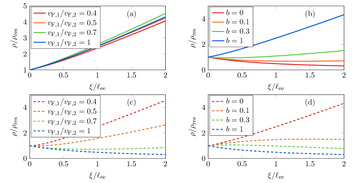
Figure 1: (a) Resistivity in the two Fermi surface model with magnetic disorder; (b) in the model (20) with magnetic disorder; (c) in the two Fermi surface model with potential disorder; (d) in the model (20) with potential disorder. Data in (c,d) is taken from [21]. Resistivities are normalized by $\rho_{\mathrm{res}}$, the ballistic residual resistivity at $\ell_{\mathrm{ee}}=\infty$. (18) leads to the blue ($v_{\mathrm{F},1}/v_{\mathrm{F,2}}=1$) curve in panels (a,b). We observe how whether electron-electron interactions enhance or suppress transport beyond the ballistic limit is sensitive to the particular hydrodynamic limit and the nature of disorder.

Let us unpack (18). In the ballistic limit $\ell_{\mathrm{ee}}\gg\xi$, $\mathcal{A}_{ij}\propto 1/k$ is essentially independent of $\ell_{\mathrm{ee}}$, as is the resistivity $\rho$. In this limit $\rho$ is the zero temperature residual resistivity: transport is dominated by single-particle motion through the random magnetic fields. The opposite limit $\ell_{\mathrm{ee}}\ll\xi$ is characterized by hydrodynamics, and so we should recover (5). We immediately observe that $\mathcal{A}_{ij}\propto 1/\ell_{\mathrm{ee}}$, consistent with (5). More quantitatively, in the model (17), one finds the shear viscosity [18, 21]

$$\eta=\frac{n^{2}\ell_{\mathrm{ee}}}{2\nu v_{\mathrm{F}}}.$$ (19)

Combining (12), (18) and (19), we indeed recover (5). Our microscopic model also allows us to quantitatively characterize the breakdown of hydrodynamic transport when $\ell_{\mathrm{ee}}\sim\xi$. Figure 1 demonstrates that even when $\ell_{\mathrm{ee}}=2\xi$, hydrodynamic effects can already double the resistivity above its residual value. Hydrodynamic effects are observable even when the condition $\ell_{\mathrm{ee}}\ll\xi$ fails.

The kinetic approach also allows us to study Fermi liquids with more complicated Fermi surfaces. In a Fermi liquid with two small Fermi surfaces of Fermi velocities $v_{\mathrm{F,1}}$ and $v_{\mathrm{F,2}}$, the quasiparticle density on each pocket are both approximately conserved [20, 21]. With this extra conservation law, the Navier-Stokes equations (2) are not applicable [21], and a more complicated (approximate) hydrodynamics emerges. Following our heuristic discussion about when $\rho\propto\ell_{\mathrm{ee}}$ vs. $\rho\propto 1/\ell_{\mathrm{ee}}$, we expect that (1) continues to hold in the hydrodynamic limit, because shear momentum is still diffusive. An explicit numerical computation in a toy model of this two-pocket Fermi liquid confirms these expectations: see Figure 1. Details of this toy model, which generalizes the single pocket model described explicitly above, are provided in Appendix D. We briefly note that for generic $v_{\mathrm{F,1}}/v_{\mathrm{F,2}}$, potential disorder also couples to a diffusive mode [21], and also leads to (1). This effect is also shown in Figure 1.

A final solvable model has [21]

$$\gamma_{n}=\frac{v_{\mathrm{F}}}{\ell_{\mathrm{ee}}}\times\left\{\begin{array}[]{ll}b&\ |n|=2\\ 1&\ |n|>2\end{array}\right..$$ (20)

We will generally take $0<b<1$, so that quadrupolar deformations of the Fermi surface are long-lived excitations. We find that (18) generalizes to

$$\mathcal{A}_{JJ}(k)=\frac{\nu}{v_{\mathrm{F}}}\frac{2b-1+\sqrt{1+k^{2}\ell_{\mathrm{ee}}^{2}}}{k^{2}\ell_{\mathrm{ee}}}.$$ (21)

Figure 1 again shows $\rho$ as a function of $b$ and $\ell_{\mathrm{ee}}$ in this model. The case $b=0$ is most interesting: here we observe that potential disorder leads to $\rho\propto 1/\ell_{\mathrm{ee}}$ while magnetic disorder leads to $\rho\propto\ell_{\mathrm{ee}}$. This unintuitive behavior is opposite of (17). To explain how this behavior follows from the conservation of quadrupolar deformations of the Fermi surface, we compute the hydrodynamic normal modes of this model in Appendix E. What we find is that the hydrodynamics of this model is rather different from (2). For wave number $\mathbf{k}=k\hat{\mathbf{x}}$, we observe two ballistically propagating modes: one coupling deformations of the Fermi surface of $p_{y}$ and $d_{xy}$ types, and another coupling $s$, $p_{x}$ and $d_{x^{2}-y^{2}}$ types. The lone diffusive mode now corresponds to out-of-phase $s$ and $d_{x^{2}-y^{2}}$ deformations. Because current/momentum couple only to ballistic modes, magnetic disorder leads to $\rho\propto\ell_{\mathrm{ee}}$; as density now couples to a diffusive mode, we find $\rho\propto 1/\ell_{\mathrm{ee}}$ with potential disorder.

In typical Fermi liquids, transverse momentum is a diffusive quantity: quadrupolar fluctuations of the Fermi surface are not typically conserved. As we detail in Appendix A, this implies that the interplay of viscous hydrodynamic and magnetic disorder will typically lead to (1), providing another route to $T^{2}$ resistivity in Fermi liquids.

Application to $\boldsymbol{\mathrm{SrTiO}_{3}}$

In this letter we have shown that (1) can result from the interplay of electron-electron interactions and the magnetic impurities. We now argue why this theory may explain the puzzling resistivity of low density $\mathrm{SrTiO}_{3}$. (i) Magnetic disorder in $\mathrm{SrTiO}_{3}$ is well-established [37, 38, 39]. (ii) Letting $\rho\approx\rho_{0}+AT^{2}$, [7] found that $A$ is insensitive to the emergence of a second band of carriers at $n\sim 10^{18}\;\mathrm{cm}^{-3}$, as is our toy model of a multi-band metal in Figure 1a. (iii) The residual resistivity $\rho_{0}$ appears unrelated to $A$ [7, 8]. In the weak disorder limit, contributions to $\rho(T)$ from magnetic vs. potential disorder add via Matthiesen’s rule. Potential disorder affects $\rho$ most strongly at low temperatures: see Figure 1c. We speculate that $\rho_{T\rightarrow 0}$ is dominated by potential disorder, while $A$ is dominated by magnetic disorder. We predict that changing the density and/or strength of magnetic/potential impurities would most strongly affect the measured coefficients of $T^{2}/T^{0}$ in $\rho(T)$, respectively. (iv) $A$ has been found to be an unconventional function of carrier density $n$ [8, 7]. Using (5) and (19), our hydrodynamic mechanism for $T^{2}$ resistivity suggests that $A\propto n_{\mathrm{imp}}\nu/n^{2}E_{\mathrm{F}}$. We propose that correlations between the amount of oxygen depletion, magnetic inhomogeneity and $n$ are responsible for the unconventional $A(n)$ observed in $\mathrm{SrTiO}_{3}$.

The resistivity of $\mathrm{SrTiO}_{3}$ can also be measured to temperature $T\gtrsim T_{\mathrm{F}}$, where thermal diffusion will also become important. A microscopic computation of the kinetic coefficients of $\mathrm{SrTiO}_{3}$ could determine the quantitative impact of this additional mode on $\rho(T)$.

Appendix A When Interactions Increase or Decrease the Resistivity

In this appendix, we use the kinetic formalism described in the main text to make the intuitive argument for when $\rho\propto\ell_{\mathrm{ee}}$ vs. $\rho\propto 1/\ell_{\mathrm{ee}}$ in the hydrodynamic regime rigorous. We decompose the set of all $|\Phi(\mathbf{p})\rangle$ into three groups such that

$$\mathsf{W} =\left(\begin{array}[]{ccc}0&\ 0&\ 0\\ 0&\ 0&\ 0\\ 0&\ 0&\ \mathsf{W}_{0}\end{array}\right),$$ (22d)

$$\mathsf{L}(\mathbf{k}) =\left(\begin{array}[]{ccc}\mathsf{L}_{1}&\ 0&\ -\mathsf{L}_{2}^{\dagger}\\ 0&\ 0&\ -\mathsf{L}_{3}^{\dagger}\\ \mathsf{L}_{2}&\ \mathsf{L}_{3}&\ \mathsf{L}_{4}\end{array}\right),$$ (22h)

with $\mathsf{L}_{1}$ invertible. The first row (I) of $|\Phi\rangle$ contains conserved quantities which mix among themselves under streaming (analogous to sound waves), the second row (II) of $|\Phi\rangle$ contains conserved quantities which only couple via streaming to non-conserved modes (purely diffusive hydrodynamic modes), and the third row (III) of $|\Phi\rangle$ corresponds to non-conserved modes. In the hydrodynamic limit $k\ell_{\mathrm{ee}}\ll 1$, using the scalings $\mathsf{L}\sim k$ and $\mathsf{W}_{0}\sim\ell_{\mathrm{ee}}^{-1}$, along with block matrix inversion identities, we find that for any vector $|\Phi\rangle$ which is entirely even or entirely odd under time reversal,

$$\langle\Phi|(\mathsf{W}+\mathsf{L})^{-1}|\Phi\rangle\lesssim\langle\Phi|\left(\begin{array}[]{ccc}\ell_{\mathrm{ee}}&\ k^{-1}&\ k^{-1}\\ k^{-1}&\ \ell_{\mathrm{ee}}^{-1}k^{-2}&\ k^{-1}\\ k^{-1}&\ k^{-1}&\ \ell_{\mathrm{ee}}\end{array}\right)|\Phi\rangle.$$ (23)

$\mathcal{A}_{ij}\sim\ell_{\mathrm{ee}}^{-1}k^{-2}$ if and only if $|\mathsf{J}_{i}\rangle$ has non-vanishing weight in block row II. In more physical terms, the current must have some overlap with a diffusive hydrodynamic mode, such as shear momentum.

The inequality in (23) – at least for the block diagonal elements – appears to be qualitatively saturated in all toy models that have been studied to date. An informal (but still rather technical) proof that this saturation is generic (and will be challenging to violate in non-pathological models) is as follows.

First, let us consider the top left block of (23), which we denote as

$$(\mathsf{W}+\mathsf{L})^{-1}_{\mathrm{I,I}}=\left(\mathsf{L}_{1}+\mathsf{L}_{2}^{\dagger}(\mathsf{W}_{0}+\mathsf{L}_{4})^{-1}\mathsf{L}_{2}\right)^{-1}\approx\left(\mathsf{L}_{1}+\mathsf{L}_{2}^{\dagger}\mathsf{W}_{0}^{-1}\mathsf{L}_{2}\right)^{-1}.$$ (24)

The approximate equality above is exact up to subleading corrections (componentwise) in $k\ell_{\mathrm{ee}}$. Because $\mathsf{L}_{1}$ is the projection of the Fourier transform of an antisymmetric matrix – $\frac{\partial\epsilon}{\partial p_{i}}\frac{\partial}{\partial x_{i}}$ projected onto conserved modes – its eigenvalues will come in pairs $\pm\mathrm{i}\lambda(\mathbf{k})$. So let us consider a basis for block row I where

$$\mathsf{L}_{1}=\mathrm{i}\left(\begin{array}[]{ccc}\lambda_{1}\sigma^{x}&\ 0&\ 0\\ 0&\ \lambda_{2}\sigma^{x}&\ \cdots\\ 0&\ \vdots&\ \ddots\end{array}\right).$$ (25)

As $\mathsf{L}_{1}$ is odd under time reversal, one of the basis vectors in each of the block rows above is odd under time reversal, and the other is even. Because $\mathsf{L}_{2}^{\dagger}\mathsf{W}_{0}^{-1}\mathsf{L}_{2}$ is symmetric and positive-definite, if there is any vector $|\Phi_{\mathrm{I}}\rangle$ obeying $\langle\Phi_{\mathrm{I}}|\mathsf{L}_{2}^{\dagger}\mathsf{W}_{0}^{-1}\mathsf{L}_{2}|\Phi_{\mathrm{I}}\rangle=0$, then $\langle\Phi_{\mathrm{I}}|\mathsf{L}_{2}^{\dagger}\mathsf{W}_{0}^{-1}\mathsf{L}_{2}|\Psi_{\mathrm{I}}\rangle=0$ for any vector $|\Psi_{\mathrm{I}}\rangle$ in the row I subspace. This identity implies that each eigenvector of $\mathsf{L}_{1}$ obeys either (i) $\langle\Phi_{\mathrm{I}}|\mathsf{L}_{2}^{\dagger}\mathsf{W}_{0}^{-1}\mathsf{L}_{2}|\Phi_{\mathrm{I}}\rangle>0$ or (ii) $\langle\Phi_{\mathrm{I}}|(\mathsf{L}_{1}+\mathsf{L}_{2}^{\dagger}\mathsf{W}_{0}^{-1}\mathsf{L}_{2})^{-1}|\Phi_{\mathrm{I}}\rangle=\langle\Phi_{\mathrm{I}}|\mathsf{L}_{1}^{-1}|\Phi_{\mathrm{I}}\rangle$. If $|\Phi_{\mathrm{I}}\rangle$ transforms with definite sign under time reversal, $\langle\Phi_{\mathrm{I}}|\mathsf{L}_{1}^{-1}|\Phi_{\mathrm{I}}\rangle=0$. In general, we do not expect modes with exactly vanishing spectral weight to exist, barring exact identities such as Ward identities (see (35) below) that demand it. We conclude that under generic circumstances, $\langle\Phi_{\mathrm{I}}|\mathsf{L}_{2}^{\dagger}\mathsf{W}_{0}^{-1}\mathsf{L}_{2}|\Phi_{\mathrm{I}}\rangle>0$. As $\mathsf{L}_{1}\sim k$ and $\mathsf{L}_{2}^{\dagger}\mathsf{W}_{0}^{-1}\mathsf{L}_{2}\sim k^{2}$, in the limit $k\rightarrow 0$ we estimate that for any $|\Phi_{\mathrm{I}}\rangle$ transforming with definite sign under time reversal,

$$\langle\Phi_{\mathrm{I}}|\left(\mathsf{L}_{1}+\mathsf{L}_{2}^{\dagger}\mathsf{W}_{0}^{-1}\mathsf{L}_{2}\right)^{-1}|\Phi_{\mathrm{I}}\rangle\sim\left(\begin{array}[]{cc}1&\ 0\end{array}\right)\left(\begin{array}[]{cc}\ell_{\mathrm{ee}}k^{2}&\ \mathrm{i}k\\ \mathrm{i}k&\ \ell_{\mathrm{ee}}k^{2}\end{array}\right)\left(\begin{array}[]{c}1\\ 0\end{array}\right)\sim\ell_{\mathrm{ee}}.$$ (26)

The remaining two blocks are much simpler. Analogously to (24), we find

$$(\mathsf{W}+\mathsf{L})^{-1}_{\mathrm{II,II}}\approx\left(\mathsf{L}_{3}^{\dagger}\mathsf{W}_{0}^{-1}\mathsf{L}_{3}\right)^{-1}.$$ (27)

The assumption that there are no non-dynamical spatial inhomogeneities in kinetic theory implies, as before, that $\mathsf{L}_{3}^{\dagger}\mathsf{W}_{0}^{-1}\mathsf{L}_{3}$ is non-singular. Using the scalings above, we arrive at $(\mathsf{W}+\mathsf{L})^{-1}_{\mathrm{II,II}}\sim\ell_{\mathrm{ee}}^{-1}k^{-2}$. Finally, in block III, $\mathsf{L}$ is negligible in the $k\rightarrow 0$ limit: $(\mathsf{W}+\mathsf{L})^{-1}_{\mathrm{III,III}}\approx\mathsf{W}_{0}^{-1}\sim\ell_{\mathrm{ee}}$.

The scalings derived above of $(\mathsf{W}+\mathsf{L})^{-1}_{\mathrm{I,I}}$ and $(\mathsf{W}+\mathsf{L})^{-1}_{\mathrm{II,II}}$ are consistent with the hydrodynamic spectral weights associated with conserved quantities that either propagate ballistically or diffusively, respectively [47, 48]; see also [21]. This explains our argument in the main text that we can check whether $\rho\propto\ell_{\mathrm{ee}}$ or $\rho\propto 1/\ell_{\mathrm{ee}}$ in the hydrodynamic limit by checking whether the impurities couple to sound waves or diffusion, respectively.

Returning to the focus of this paper on magnetic disorder, it remains to understand whether the current operator is generically contained within blocks I, II, and/or III. The key observation is that at finite density, the current $|\mathsf{J}_{i}\rangle$ always overlaps with momentum $|\mathsf{P}_{i}\rangle$: for a precise statement, see (32a) below. Transverse momentum $|\mathsf{P}_{i}\rangle$, obeying $k_{i}|\mathsf{P}_{i}\rangle=0$, often only couples to non-conserved modes, and is therefore in block II.

In some model Fermi liquids, it may be possible to explicitly prove that transverse momentum is diffusive (in block II) using group theory. As an example, suppose that all inversion-even conserved quantities $|\rho\rangle$ transform in the trivial representation $\mathbf{1}$ of the point group $G$ of the crystal, while $|\mathsf{P}_{i}\rangle$ and $|\mathsf{J}_{i}\rangle$ transform in represetation $\mathbf{V}$. Note that $\epsilon(\mathbf{p})$, $f_{\mathrm{eq}}$ and the inner product (11) are invariant under the action of $G$ on $\mathbf{p}$, so the overlap of $|\mathsf{J}_{i}\rangle$ and $|\mathsf{P}_{i}\rangle$ implies they transform in the same representation (see Section 7.1 of [49]). The same orthogonality theorems also imply that $\mathbf{V}\otimes\mathbf{V}=\mathbf{1}\oplus\cdots$ contain exactly one copy of the trivial representation $\mathbf{1}$, and that

$$\langle\rho|\mathsf{L}(k_{i})|\mathsf{P}_{j}\rangle\sim\text{\mbox{\hskip 4.44444pt{1 0 -.18 1}\hbox to0.0pt{\hss\leavevmode\hbox{\set@color$\delta$}}}}_{ij},$$ (28)

and inversion symmetry demands that $\mathsf{L}(k_{i})|\mathsf{P}_{j}\rangle$ has no overlap with any inversion odd basis vectors. We conclude that the streaming terms $\mathsf{L}$ couple transverse momenta only to non-conserved inversion-even modes. Conservation of transverse momentum, together with (23), implies (1).

In the model (20) with $b=0$, the conserved $|\pm 2\rangle$ modes are inversion even, and so the paragraph above does not apply. However, the group theoretical arguments above suffice to show that the interplay of magnetic disorder and hydrodynamic effects lead to (1) in many anisotropic electron fluids.

Appendix B Resistivity from the Boltzmann Equation

In this appendix, we derive (12) and (13), following [21]. The logic follows the hydrodynamic derivation of (5). We begin by noting that when $B_{ij}=0$ and $E_{i}=0$, an exact time-independent solution to (9) is

$$|\Phi\rangle=\alpha_{i}|\mathsf{P}_{i}\rangle,$$ (29)

where $|\mathsf{P}_{i}\rangle=\int\mathrm{d}^{d}\mathbf{p}\;p_{i}|\mathbf{p}\rangle$, for any $\alpha$. Our goal is now to show that when $E_{i}\neq 0$ and $B_{ij}\neq 0$, then we can perturbatively construct a solution to (9), analogous to the Navier-Stokes equations, starting from (29). We write

$$|\Phi\rangle=\alpha_{i}|\mathsf{P}_{i}\rangle+|\Phi_{1}(\mathbf{x})\rangle+\cdots$$ (30)

with $\alpha_{i}\sim\delta^{-2}$, $|\Phi_{1}\rangle\sim\delta^{-1}$, etc. The Fourier transform of (9) at $\mathrm{O}(\delta^{-1})$ reads

$$(\mathsf{W}+\mathsf{L}(\mathbf{k}))|\Phi_{1}(\mathbf{k})\rangle=e\frac{\partial\epsilon}{\partial p_{i}}B_{ij}(\mathbf{k})\alpha_{j}|\mathsf{n}\rangle=-\alpha_{j}B_{ij}(\mathbf{k})|\mathsf{J}_{i}\rangle.$$ (31)

where $|\mathsf{n}\rangle=\int\mathrm{d}^{d}\mathbf{p}\;|\mathbf{p}\rangle$ corresponds to the vector associated with density fluctuations in the distribution function. At $\mathrm{O}(\delta^{0})$, we spatially integrate (9), sandwiched with the bra $\langle\mathsf{P}_{k}|$, to fix $\alpha_{i}$. Using the identities

$$\langle\mathsf{J}_{i}|\mathsf{P}_{j}\rangle =-e\int\frac{\mathrm{d}^{d}\mathbf{p}}{(2\text{\mbox{\hskip 5.70027pt{1 0 -.18 1}\hbox to0.0pt{\hss\leavevmode\hbox{\set@color$\pi$}}}}\hbar)^{d}}\left(-\frac{\partial f_{\mathrm{eq}}}{\partial\epsilon}\frac{\partial\epsilon}{\partial p_{i}}\right)p_{j}=-e\int\frac{\mathrm{d}^{d}\mathbf{p}}{(2\text{\mbox{\hskip 5.70027pt{1 0 -.18 1}\hbox to0.0pt{\hss\leavevmode\hbox{\set@color$\pi$}}}}\hbar)^{d}}f_{\mathrm{eq}}\frac{\partial p_{j}}{\partial p_{i}}=-en\text{\mbox{\hskip 4.44444pt{1 0 -.18 1}\hbox to0.0pt{\hss\leavevmode\hbox{\set@color$\delta$}}}}_{ij},$$ (32a)

$$\left\langle\mathsf{P}_{k}\left|\frac{\partial\epsilon}{\partial p_{i}}B_{ij}(\mathbf{k})\frac{\partial}{\partial p_{j}}\right|\Phi\right\rangle =\int\frac{\mathrm{d}^{d}\mathbf{p}}{(2\text{\mbox{\hskip 5.70027pt{1 0 -.18 1}\hbox to0.0pt{\hss\leavevmode\hbox{\set@color$\pi$}}}}\hbar)^{d}}f_{\mathrm{eq}}\frac{\partial}{\partial p_{i}}\left(B_{ij}(\mathbf{k})p_{k}\frac{\partial\Phi}{\partial p_{j}}\right)=\int\frac{\mathrm{d}^{d}\mathbf{p}}{(2\text{\mbox{\hskip 5.70027pt{1 0 -.18 1}\hbox to0.0pt{\hss\leavevmode\hbox{\set@color$\pi$}}}}\hbar)^{d}}f_{\mathrm{eq}}B_{kj}(\mathbf{k})\frac{\partial\Phi_{2}}{\partial p_{j}}$$

$$=\int\frac{\mathrm{d}^{d}\mathbf{p}}{(2\text{\mbox{\hskip 5.70027pt{1 0 -.18 1}\hbox to0.0pt{\hss\leavevmode\hbox{\set@color$\pi$}}}}\hbar)^{d}}\left(-\frac{\partial f_{\mathrm{eq}}}{\partial\epsilon}\right)\frac{\partial\epsilon}{\partial p_{j}}B_{kj}(\mathbf{k})\Phi_{2}=-\frac{1}{e}\langle\mathsf{J}_{j}|B_{jk}(\mathbf{k})|\Phi\rangle,$$ (32b)

we find

$$\langle\mathsf{P}_{k}|E_{i}|\mathsf{J}_{i}\rangle=-enE_{k}=\int\frac{\mathrm{d}^{d}\mathbf{k}}{(2\text{\mbox{\hskip 5.70027pt{1 0 -.18 1}\hbox to0.0pt{\hss\leavevmode\hbox{\set@color$\pi$}}}})^{d}}B_{ij}(-\mathbf{k})\langle\mathsf{J}_{j}|\Phi_{1}(\mathbf{k})\rangle=\alpha_{k}\int\frac{\mathrm{d}^{d}\mathbf{k}}{(2\text{\mbox{\hskip 5.70027pt{1 0 -.18 1}\hbox to0.0pt{\hss\leavevmode\hbox{\set@color$\pi$}}}})^{d}}B_{ij}(-\mathbf{k})B_{kl}(\mathbf{k})\mathcal{A}_{jl}(\mathbf{k}).$$ (33)

The spatially averaged current is – by definition – given by $J^{\mathrm{avg}}_{i}=\langle\mathsf{J}_{i}|\Phi\rangle$. To leading order,

$$J^{\mathrm{avg}}_{i}=\alpha_{k}\langle\mathsf{J}_{i}|\mathsf{P}_{k}\rangle=-en\alpha_{i}.$$ (34)

Combining (33) and (34), we obtain (13).

Using the Ward identity

$$k_{i}\mathcal{A}_{ij}(\mathbf{k})=k_{j}\mathcal{A}_{ij}(\mathbf{k})=0,$$ (35)

we obtain the result predicted by the memory matrix formalism [41, 42, 43]:

$$\rho_{ij}=\frac{1}{e^{2}n^{2}}\int\frac{\mathrm{d}^{d}\mathbf{k}}{(2\text{\mbox{\hskip 5.70027pt{1 0 -.18 1}\hbox to0.0pt{\hss\leavevmode\hbox{\set@color$\pi$}}}})^{d}}k_{i}k_{j}a_{k}(-\mathbf{k})a_{l}(\mathbf{k})\mathcal{A}_{kl}(\mathbf{k}),$$ (36)

Appendix C Magnetic Fields from Random Magnetic Dipoles

In this appendix we explicitly derive (14). For a magnetic dipole of strength $\mathfrak{m}\hat{\mathbf{z}}$ located a distance $\xi$ above a two dimensional plane at the point $(x,y,z)=(0,0,\xi)$, the magnetic vector potential lies entirely within the $xy$ plane. Tthe $x$ and $y$ components of this vector potential are given by

$$A_{i}=\frac{\mu_{0}\mathfrak{m}}{4\text{\mbox{\hskip 5.70027pt{1 0 -.18 1}\hbox to0.0pt{\hss\leavevmode\hbox{\set@color$\pi$}}}}}\frac{-\epsilon_{ij}x_{j}}{(r^{2}+\xi^{2})^{3/2}}=-\frac{\mu_{0}\mathfrak{m}}{4\text{\mbox{\hskip 5.70027pt{1 0 -.18 1}\hbox to0.0pt{\hss\leavevmode\hbox{\set@color$\pi$}}}}}\epsilon_{ij}\frac{\partial}{\partial x_{j}}\frac{1}{\sqrt{r^{2}+\xi^{2}}}.$$ (37)

Our first goal is to Fourier transform $A_{i}$ in the $xy$ plane. It is easier to “guess” the transform $A_{i}(\mathbf{k})$ and check that the Fourier transform of $A_{i}(\mathbf{k})$ is (37). Our “guess” for the Fourier transform is

$$A_{i}(\mathbf{k})=-\mathrm{i}\frac{\mu_{0}\mathfrak{m}}{2}\epsilon_{ij}\frac{k_{j}}{k}\mathrm{e}^{-k\xi},$$ (38)

where we have denoted $k=|\mathbf{k}|$. The Fourier transform of $A_{i}(\mathbf{k})$ can be analytically computed:

$$A_{i}(\mathbf{x}) =\int\frac{\mathrm{d}^{2}\mathbf{k}}{(2\text{\mbox{\hskip 5.70027pt{1 0 -.18 1}\hbox to0.0pt{\hss\leavevmode\hbox{\set@color$\pi$}}}})^{2}}\left(-\mathrm{i}\frac{\mu_{0}\mathfrak{m}}{2}\epsilon_{ij}\frac{k_{j}}{k}\mathrm{e}^{-k\xi}\right)\mathrm{e}^{\mathrm{i}\mathbf{k}\cdot\mathbf{x}}=-\frac{\partial}{\partial x_{j}}\epsilon_{ij}\int\frac{\mathrm{d}^{2}\mathbf{k}}{(2\text{\mbox{\hskip 5.70027pt{1 0 -.18 1}\hbox to0.0pt{\hss\leavevmode\hbox{\set@color$\pi$}}}})^{2}}\frac{\mu_{0}\mathfrak{m}}{2}\frac{\mathrm{e}^{-k\xi}}{k}$$

$$=-\frac{\partial}{\partial x_{j}}\epsilon_{ij}\frac{\mu_{0}\mathfrak{m}}{4\text{\mbox{\hskip 5.70027pt{1 0 -.18 1}\hbox to0.0pt{\hss\leavevmode\hbox{\set@color$\pi$}}}}}\int\limits_{0}^{2\text{\mbox{\hskip 3.99019pt{1 0 -.18 1}\hbox to0.0pt{\hss\leavevmode\hbox{\set@color$\pi$}}}}}\frac{\mathrm{d}\theta}{2\text{\mbox{\hskip 5.70027pt{1 0 -.18 1}\hbox to0.0pt{\hss\leavevmode\hbox{\set@color$\pi$}}}}}\int\limits_{0}^{\infty}\mathrm{d}k\mathrm{e}^{\mathrm{i}kr\cos\theta-k\xi}=-\frac{\partial}{\partial x_{j}}\epsilon_{ij}\frac{\mu_{0}\mathfrak{m}}{4\text{\mbox{\hskip 5.70027pt{1 0 -.18 1}\hbox to0.0pt{\hss\leavevmode\hbox{\set@color$\pi$}}}}}\int\limits_{0}^{2\text{\mbox{\hskip 3.99019pt{1 0 -.18 1}\hbox to0.0pt{\hss\leavevmode\hbox{\set@color$\pi$}}}}}\frac{\mathrm{d}\theta}{2\text{\mbox{\hskip 5.70027pt{1 0 -.18 1}\hbox to0.0pt{\hss\leavevmode\hbox{\set@color$\pi$}}}}}\frac{1}{\xi-\mathrm{i}r\cos\theta}.$$ (39)

This final integral can be done via contour integration, and one indeed recovers (37). In two dimensions, the Fourier transform of the magnetic field $B_{ij}=\mathrm{i}k_{i}A_{j}-\mathrm{i}k_{j}A_{i}\equiv B\epsilon_{ij}$, where

$$B=\mathrm{i}\epsilon_{ij}k_{i}A_{j}=\frac{\mu_{0}\mathfrak{m}}{2}k\mathrm{e}^{-k\xi}.$$ (40)

If, instead of being located above the origin, the magnetic dipole is located at the point $(x,y,\xi)$, then we simplify multiply $A_{i}(\mathbf{k})$ by a factor of $\mathbf{e}^{\mathrm{i}(k_{x}x+k_{y}y)}$. If we have multiple magnetic dipoles located at points $\mathbf{r}_{a}$, then

$$A_{i}(\mathbf{k})=\mathrm{i}\frac{\mu_{0}\mathfrak{m}}{2}\epsilon_{ij}\frac{k_{j}}{k}\mathrm{e}^{-k\xi}\sum_{a}\mathrm{e}^{\mathrm{i}\mathbf{k}\cdot\mathbf{r}_{a}}.$$ (41)

So before disorder averaging, the magnetic fields in (12) take the form

$$B_{ij}(-\mathbf{k})B_{kl}(\mathbf{k})=\epsilon_{ij}\epsilon_{kl}\left(\frac{\mu_{0}\mathfrak{m}}{2}\right)^{2}k^{2}\mathrm{e}^{-2k\xi}\sum_{a,b}\mathrm{e}^{\mathrm{i}\mathbf{k}\cdot(\mathbf{r}_{a}-\mathbf{r}_{b})}.$$ (42)

Disorder averaging corresponds to spatially averaging over all possible positions of $\mathbf{r}_{a}$ for each $a$:

$$\langle F\rangle_{\mathrm{dis}}=\int\left(\prod_{a}\frac{\mathrm{d}^{2}\mathbf{r}_{a}}{V}\right)F.$$ (43)

where $V$ is the volume of the sample. The only non-vanishing terms in $\langle B_{ij}(-\mathbf{k})B_{kl}(\mathbf{k})\rangle_{\mathrm{dis}}$ correspond to $a=b$. If there are $N_{\mathrm{imp}}=n_{\mathrm{imp}}V$ total impurities in the volume $V$, we conclude that

$$\langle B_{ij}(-\mathbf{k})B_{kl}(\mathbf{k})\rangle_{\mathrm{dis}}=\epsilon_{ij}\epsilon_{kl}\left(\frac{\mu_{0}\mathfrak{m}}{2}\right)^{2}k^{2}\mathrm{e}^{-2k\xi}\times\frac{N_{\mathrm{imp}}}{V}$$ (44)

which is equivalent to (14).

Appendix D A Model of Two Fermi Surfaces

We review the model of two Fermi surfaces described in [21]. For simplicity, we assume that the density of states of each Fermi surface is the same, $\nu$. We also assume that each band has a quadratic dispersion relation with the same mass $m$, so that the current and momentum of each band separately are proportional to each other. If there are two circular Fermi surfaces, then we may generalize the logic of the main text to replace (15) with

$$|\Phi\rangle=\sum_{A=1}^{2}\sum_{n\in\mathbb{Z}}a_{nA}|nA\rangle.$$ (45)

in the low temperature limit. The index $A=1,2$ denotes which one of the two Fermi surfaces carries a fluctuation. The streaming matrix is

$$\mathsf{L}|nA\rangle=\frac{v_{\mathrm{F}}}{2}(\mathrm{i}k_{x}-k_{y})|(n+1)A\rangle+\frac{v_{\mathrm{F}}}{2}(\mathrm{i}k_{x}+k_{y})|(n-1)A\rangle,$$ (46)

and the collision matrix is

$$\mathsf{W}=\frac{v_{\mathrm{F2}}}{\nu\ell_{\mathrm{ee}}}\left[\sum_{A,|j|\geq 2}|jA\rangle\langle jA|+\sum_{j=\pm 1}\frac{(v_{\mathrm{F2}}|j1\rangle-v_{\mathrm{F1}}|j2\rangle)(v_{\mathrm{F2}}\langle j1|-v_{\mathrm{F1}}\langle j2|)}{v_{\mathrm{F1}}^{2}+v_{\mathrm{F2}}^{2}}\right]$$ (47)

The factor of $\nu$ is required due to the non-trivial inner product (11).

In this model, the total momentum is simply given by the momentum carried in each band. With the dispersion relation described above, we find that the total momentum and current are proportional, and given by [21]

$$|\mathsf{J}_{x}\rangle\pm\mathrm{i}|\mathsf{J}_{y}\rangle\equiv|\mathsf{J}_{\pm}\rangle=-ev_{\mathrm{F,1}}|\pm 1,1\rangle-ev_{\mathrm{F,2}}|\pm 1,2\rangle.$$ (48)

The techniques to compute $\langle\mathsf{J}_{i}|(\mathsf{W}+\mathsf{L})^{-1}|\mathsf{J}_{j}\rangle$ are detailed in [17, 18, 21]. They amount to a more souped up version of the following argument, which is sufficient to understand the hydrodynamic limit. Consider the block matrix inversion identity

$$\left(\begin{array}[]{cc}\mathbf{v}^{\mathsf{T}}&\ 0\end{array}\right)\left(\begin{array}[]{cc}\mathsf{A}&\ \mathsf{B}\\ \mathsf{C}&\ \mathsf{D}\end{array}\right)^{-1}\left(\begin{array}[]{c}\mathbf{w}\\ 0\end{array}\right)=\mathbf{v}^{\mathsf{T}}\left(\mathsf{A}-\mathsf{BD}^{-1}\mathsf{C}\right)^{-1}\mathbf{w}.$$ (49)

We arrange the infinite dimensional vector space spanned by $|nA\rangle$ such that the modes $|jA\rangle$ with $|j|\leq 1$ are in the top block, and modes with $|j|>1$ are in the bottom block. Using (46) and (47), we see that to leading order as $k\rightarrow 0$, the inverse of $\mathsf{W}+\mathsf{L}$ in the bottom block is simply $\mathsf{W}^{-1}$: accounting for $\mathsf{L}$ leads to subleading corrections in $k$. Inverting the remaining $6\times 6$ matrix and keeping only the leading order terms as $k\rightarrow 0$, we obtain

$$\mathcal{A}_{ij}(k)=\frac{2e^{2}v_{\mathrm{F,2}}\left(v_{\mathrm{F,1}}^{2}+v_{\mathrm{F,2}}^{2}\right)^{2}}{\ell_{\mathrm{ee}}\left(v_{\mathrm{F,1}}^{4}+v_{\mathrm{F,2}}^{4}\right)k^{2}}\left(\text{\mbox{\hskip 4.44444pt{1 0 -.18 1}\hbox to0.0pt{\hss\leavevmode\hbox{\set@color$\delta$}}}}_{ij}-\frac{k_{i}k_{j}}{k^{2}}\right),$$ (50)

which has the expected $k^{-2}$ dependence arising from transverse momentum diffusion. Using the generalized techniques of [17, 18, 21], we have numerically evaluated $\mathcal{A}_{ij}$ for any value of $k\ell_{\mathrm{ee}}$. This result is plotted in Figure 1 of the main text.

Appendix E Normal Modes When $b=0$

In this appendix, we explicitly give the approximate eigenvalues and eigenvectors of $\mathsf{W}+\mathsf{L}(\mathbf{k})$, corresponding to the gapless hydrodynamic modes. The techniques to derive this result are analogous to those used to derive (50); for this model, the “top block” of (49) consists of modes with $|j|\leq 2$. Without loss of generality, we take $k_{x}=k$, $k_{y}=0$. In the hydrodynamic limit $k\ell_{\mathrm{ee}}\rightarrow 0$, we find

$$\omega =\pm\frac{v_{\mathrm{F}}}{2}k+\cdots,\;\;\;\;\;\text{eigenvector}=|2\rangle\pm|1\rangle\mp|-1\rangle-|-2\rangle,$$ (51a)

$$\omega =\pm\frac{\sqrt{3}v_{\mathrm{F}}}{2}k+\cdots,\;\;\;\;\;\text{eigenvector}=|2\rangle\pm\sqrt{3}|1\rangle+2|0\rangle\pm\sqrt{3}|-1\rangle+|-2\rangle,$$ (51b)

$$\omega =-\mathrm{i}\frac{v_{\mathrm{F}}^{2}}{6\gamma}k^{2}+\cdots,\;\;\;\;\;\text{eigenvector}=|2\rangle-|0\rangle+|-2\rangle.$$ (51c)

Note that there are no hydrodynamic modes involving $|j\rangle$ for $|j|>2$ – all of these modes have a finite lifetime $\omega\approx-\mathrm{i}v_{\mathrm{F}}/\ell_{\mathrm{ee}}$. We observe that the current modes $|\pm 1\rangle$ are only included in ballistically propgating modes (generalized “sound waves”). So, as asserted in the main text, random magnetic fields do not excite diffusive fluctuations, and this is why $\rho\propto\ell_{\mathrm{ee}}$ in this model. In contrast, chemical potential disorder couples to $|0\rangle$, not $|\pm 1\rangle$. $|0\rangle$ does have overlap with the diffusive mode above, and this is why (as shown in Figure 1), potential disorder leads to (1) in this model.

References

- [1] K. Kadowaki and S. B. Woods. “Universal relationship of the resistivity and specific heat in heavy-fermion compounds”, Solid State Communications 58 507 (1987).
- [2] A. C. Jacko, J. O. Fjaerestad, and B. J. Powell. “Unified explanation of the Kadowaki-Woods ratio in strongly correlated materials”, Nature Physics 5 422 (2009), arXiv:0805.4275.
- [3] J. A. N. Bruin, H. Sakai, R. S. Perry, and A. P. Mackenzie. “Similarity of scattering rates in metals showing -linear resistivity”, Science 339 804 (2013).
- [4] S. A. Hartnoll. “Theory of universal incoherent metallic transport”, Nature Physics 11 54 (2015), arXiv:1405.3651.
- [5] J. Ziman. Electrons and Phonons (Oxford University Press, 1960).
- [6] W. G. Baber. “The contribution to the electrical resistance of metals from collisions between electrons”, Proceedings of the Royal Society A158 383 (1937).
- [7] X. Lin, B. Fauque, and K. Behnia. “Scalable resistivity in a small single-component Fermi surface”, Science 349 945 (2015), arXiv:1508.07812.
- [8] E. Mikheev, S. Raghavan, J. Y. Zhang, P. B. Marshall, A. P. Kajdos, L. Balents, and S. Stemmer. “Carrier density independent scattering rate in -based electron liquids”, Scientific Reports 6 20865 (2016), arXiv:1512.02294.
- [9] R. N. Gurzhi. “Minimum of resistance in impurity-free conductors”, Journal of Experimental and Theoretical Physics 17 521 (1963).
- [10] M. Hruska and B. Spivak. “Conductivity of the classical two-dimensional electron gas”, Physical Review B65 033315 (2002), arXiv:cond-mat/0102219.
- [11] A. V. Andreev, S. A. Kivelson, and B. Spivak. “Hydrodynamic description of transport in strongly correlated electron systems”, Physical Review Letters 106 256804 (2011), arXiv:1011.3068.
- [12] A. Lucas. “Hydrodynamic transport in strongly coupled disordered quantum field theories”, New Journal of Physics 17 113007 (2015), arXiv:1506.02662.
- [13] I. Torre, A. Tomadin, A. K. Geim, and M. Polini. “Non-local transport and the hydrodynamic shear viscosity in graphene”, Physical Review B92 165433 (2016), arXiv:1508.00363.
- [14] L. Levitov and G. Falkovich. “Electron viscosity, current vortices and negative nonlocal resistance in graphene”, Nature Physics 12 672 (2016), arXiv:1508.00836.
- [15] A. Lucas, J. Crossno, K. C. Fong, P. Kim, and S. Sachdev. “Transport in inhomogeneous quantum critical fluids and in the Dirac fluid in graphene”, Physical Review B93 075426 (2016), arXiv:1510.01738.
- [16] P. S. Alekseev. “Negative magnetoresistance in viscous flow of two-dimensional electrons”, Physical Review Letters 117 166601 (2016).
- [17] H. Guo, E. Ilseven, G. Falkovich, and L. Levitov. “Higher-than-ballistic conduction of viscous electron flows”, Proceedings of the National Academy of Sciences 114 3068 (2017), arXiv:1607.07269.
- [18] A. Lucas. “Stokes paradox in electronic Fermi liquids”, Physical Review B95 115425 (2017), arXiv:1612.00856.
- [19] H. Guo, E. Ilseven, G. Falkovich, and L. Levitov. “Stokes paradox, back reflections and interaction-enhanced conductance”, arXiv:1612.09239.
- [20] A. Lucas and S. A. Hartnoll. “Resistivity bound for hydrodynamic bad metals”, arXiv:1704.07384.
- [21] A. Lucas and S. A. Hartnoll. “Kinetic theory of transport for inhomogeneous electron fluids”, arXiv:1706.04621.
- [22] A. Lucas and K. C. Fong. “Hydrodynamics of electrons in graphene”, arXiv:1710.08425.
- [23] M. J. M. de Jong and L. W. Molenkamp. “Hydrodynamic electron flow in high-mobility wires”, Physical Review B51 11389 (1995), arXiv:cond-mat/9411067.
- [24] D. A. Bandurin et al. “Negative local resistance due to viscous electron backflow in graphene”, Science 351 1055 (2016), arXiv:1509.04165.
- [25] J. Crossno et al. “Observation of the Dirac fluid and the breakdown of the Wiedemann-Franz law in graphene”, Science 351 1058 (2016), arXiv:1509.04713.
- [26] P. J. W. Moll, P. Kushwaha, N. Nandi, B. Schmidt, and A. P. Mackenzie. “Evidence for hydrodynamic electron flow in ”, Science 351 1061 (2016), arXiv:1509.05691.
- [27] J. Gooth, F. Menges, C. Shekhar, V. Süss, N. Kumar, Y. Sun, U. Drechsler, R. Zierold, C. Felser, and B. Gotsmann. “Electrical and thermal transport at the Planckian bound of dissipation in the hydrodynamic electron fluid of ”, arXiv:1706.05925.
- [28] D. S. Novikov. “Viscosity of a two-dimensional Fermi liquid”, arXiv:cond-mat/0603184.
- [29] R. Krishna Kumar et al. “Super-ballistic flow of viscous electron fluid through graphene constrictions”, arXiv:1703.06672.
- [30] Q. Shi, P. D. Martin, Q. A. Ebner, M. A. Zudov, L. N. Pfeiffer, and K. W. West. “Colossal negative magnetoresistance in a two-dimensional electron gas”, Physical Review B89 201301 (2014).
- [31] S. Doniach. “The Kondo lattice and weak antiferromagnetism”, Physica B91 231 (1977).
- [32] P. Aynajian, E. H. da Silva Neto, A. Gyenis, R. E. Baumbach, J. D. Thompson, Z. Fisk, E. D. Bauer, and A. Yazdani. “Visualizing heavy fermions emerging in a quantum critical Kondo lattice”, Nature 486 201 (2012), arXiv:1206.3145.
- [33] Y. P. Wu, D. Zhao, A. F. Wang, N. Z. Wang, Z. J. Xiang, X. G. Luo, T. Wu, and X. H. Chen. “Emergent Kondo lattice behavior in iron-based superconductors (, Rb, Cs)”, Physical Review Letters 116 147001 (2016), arXiv:1507.08732.
- [34] H. Alloul, P. Mendels, H. Casalta, J. F. Marucco, and J. Arabski. “Correlations between magnetic and superconducting properties of Zn-substituted ”, Physical Review Letters 67 3140 (1991).
- [35] P. Mendels, J. Bobroff, G. Collin, H. Alloul, M. Gabay, J. F. Marucco, N. Blanchard, and B. Greiner. “Normal-state magnetic properties of Ni and Zn substituted in : hole-doping dependence”, Europhysics Letters 46 678 (1999).
- [36] A. V. Balatsky, I. Vekhter, and J-X. Zhu. “Impurity-induced states in conventional and unconventional superconductors”, Reviews of Modern Physics 78 373 (2006), arXiv:cond-mat/0411318.
- [37] A. Brinkman, M. Huijben, M. van Zalk, J. Huijben, U. Zeitler, J. C. Maan, W. G. van der Wiel, G. Rijnders, D. H. A. Blank, and H. Hilgenkamp. “Magnetic effects at the interface between nonmagnetic oxides”, Nature Materials 6 493 (2007), arXiv:cond-mat/0703028.
- [38] M. Lee, J. R. Williams, S. Zhang, C. D. Frisbie, and D. Goldhaber-Gordon. “Electrolyte gate-controlled Kondo effect in ”, Physical Review Letters 107 256601 (2011), arXiv:1108.0139.
- [39] B. Kalisky, J. A. Bert, C. Bell, Y. Xie, H. K. Sato, M. Hosoda, Y. Hikita, H. Y. Hwang, and K. A. Moler. “Scanning probe manipulation of magnetism at the heterointerface”, Nano Letters 12 4055 (2012).
- [40] A. Kamenev. Field Theory of Non-Equilibrium Systems (Cambridge University Press, 2011).
- [41] S. A. Hartnoll and D. M. Hofman. “Locally critical umklapp scattering and holography”, Physical Review Letters 108 241601 (2012), arXiv:1201.3917.
- [42] A. Lucas and S. Sachdev. “Memory matrix theory of magnetotransport in strange metals”, Physical Review B91 195122 (2015), arXiv:1502.04704.
- [43] S. A. Hartnoll, A. Lucas, and S. Sachdev. “Holographic quantum matter”, arXiv:1612.07324.
- [44] P. L. Bhatnagar, E. P. Gross, and M. Krook. “A model for collision processes in gases. I. Small amplitude processes in charged and neutral one-component systems”, Physical Review 94 511 (1954).
- [45] P. Ledwith, H. Guo, and L. Levitov. “Fermion collisions in two dimensions”, arXiv:1708.01915.
- [46] P. Ledwith, H. Guo, A. V. Shytov, and L. Levitov. “Head-on collisions and scale-dependent viscosity in two-dimensional electron systems”, arXiv:1708.02376.
- [47] L. P. Kadanoff and P. C. Martin. “Hydrodynamic equations and correlation functions”, Annals of Physics 24 419 (1963).
- [48] P. Kovtun. “Lectures on hydrodynamic fluctuations in relativistic theories”, Journal of Physics A45 473001 (2012), arXiv:1205.5040.
- [49] M. S. Dresselhaus, G. Dresselhaus, and A. Jorio. Group Theory: Application to the Physics of Condensed Matter, (Springer, 2010).