Linear models for systematics and nuisances

1 Introduction

The target of many astronomical studies is the recovery of tiny astrophysical signals living in a sea of uninteresting (but usually dominant) noise. In many contexts (i.e., stellar time-series, or high-contrast imaging, or stellar spectroscopy), there are structured components in this noise caused by systematic effects in the astronomical source, the atmosphere, the telescope, or the detector. More often than not, evaluation of the true physical model for these nuisances is computationally intractable and dependent on too many (unknown) parameters to allow rigorous probabilistic inference.

Sometimes, housekeeping data—and often the science data themselves—can be used as predictors of the systematic noise. Linear combinations of these predictors (or linear combinations of non-linear functions of these predictors) are often used as computationally tractable models that can capture the nuisances. These models can be used to fit and subtract systematics prior to investigation of the signals of interest, or they can be used in a simultaneous fit of the systematics and the signals. For our purposes, a linear model for a column vector of data ${\boldsymbol{y}}$ can be written in the form

$${\boldsymbol{y}}={\boldsymbol{\mu}}({\boldsymbol{\theta}})+{\boldsymbol{A}}{\boldsymbol{w}}+\mathrm{noise}$$ (1)

where ${\boldsymbol{\mu}}({\boldsymbol{\theta}})$ is the column vector expectation or mean model (the part of the model that we care about), ${\boldsymbol{A}}$ is a design matrix, whose columns are basis vectors (predictors) for the systematics, and ${\boldsymbol{w}}$ is the vector of weights or amplitudes, one for each basis vector.

Similar models have been used to describe the systematics in astrophysical time series data (Smith et al., 2012; Wang et al., 2016; Luger et al., 2016), galaxy or stellar spectra (Tsalmantza & Hogg, 2012; Ness et al., 2015), and imaging (Fergus et al., 2014; Wang et al., 2017). One issue with flexible data-driven models is their tendency to overfit and reduce the astrophysical signal of interest. This is generally tackled using a dimensionality reduction technique like principal component analysis (PCA) or by applying strong priors or a regularization to the weights vector ${\boldsymbol{w}}$.

In this Note, we show that if a Gaussian prior is placed on the weights ${\boldsymbol{w}}$ of the linear components, the weights can be marginalized out with an operation in pure linear algebra, which can (often) be made fast. We illustrate this model by demonstrating the applicability of a linear model for the non-linear systematics in K2 time-series data, where the dominant noise source for many stars is spacecraft motion and variability.

2 The problem

Consider a dataset ${\boldsymbol{y}}$ of $N$ measurements $y_{i}$ with covariance matrix ${\boldsymbol{C}}$. In the common case of data collected with measurement error $\sigma_{i}$ on individual data points but no correlation across measurements, ${\boldsymbol{C}}$ is a diagonal matrix with ${\boldsymbol{C}}_{ij}=\sigma_{i}\delta_{ij}$, although in general the off-diagonal elements capture the covariance between different measurements. Given a linear model as in Equation (1), the probability of the data under the model is given by a normal distribution with mean ${\boldsymbol{\mu}}({\boldsymbol{\theta}})+{\boldsymbol{A}}{\boldsymbol{w}}$ and covariance ${\boldsymbol{C}}$:

$$p({\boldsymbol{y}}|{\boldsymbol{\theta}},{\boldsymbol{w}}) =\mathcal{N}({\boldsymbol{y}};{\boldsymbol{\mu}}({\boldsymbol{\theta}})+{\boldsymbol{A}}{\boldsymbol{w}},{\boldsymbol{C}})\quad.$$ (2)

However, we are specifically not interested in the value of ${\boldsymbol{w}}$. Instead, we will marginalize over it. To perform this marginalization we must place a prior on ${\boldsymbol{w}}$ that we will assume to be Gaussian:

$$p({\boldsymbol{w}}) =\mathcal{N}({\boldsymbol{w}};0,{\boldsymbol{\Lambda}})\quad.$$

With this prior and the likelihood in Equation (2), our goal is to marginalize out the weights ${\boldsymbol{w}}$; that is, we want to compute the marginalized likelihood,

$$p({\boldsymbol{y}}|{\boldsymbol{\theta}}) =\int_{-\infty}^{\infty}p({\boldsymbol{w}})\,p({\boldsymbol{y}}|{\boldsymbol{\theta}},{\boldsymbol{w}})\mathrm{d}{\boldsymbol{w}}\quad.$$ (3)

In doing so, we would like to avoid explicitly solving for the weights ${\boldsymbol{w}}$ while also avoiding the evaluation of numerical integrals.

3 The solution

As we show in the Appendix, the marginalized likelihood (Equation 3) may be expressed as:

$$p({\boldsymbol{y}}|{\boldsymbol{\theta}})=\mathcal{N}({\boldsymbol{y}};{\boldsymbol{\mu}}({\boldsymbol{\theta}}),{\boldsymbol{C}}+{\boldsymbol{A}}{\boldsymbol{\Lambda}}{\boldsymbol{A}}^{\top})\quad.$$ (4)

This marginalized likelihood function can be numerically maximized to find the maximum likelihood parameters $\theta^{\star}$, or it can be multiplied by a prior $p(\theta)$ and used for posterior inference. In either case, the evaluation of the model will include the effects of marginalizing over ${\boldsymbol{w}}$ in the linear model and any uncertainties in those values will be propagated to the results.

It is often useful to compute the value of the linear model so that we can “remove” systematics from the data. To derive this, we recognize that Equation (4) is the likelihood of a Gaussian Process. This means that conditioned on the data and a choice of the parameters ${\boldsymbol{\theta}}$, the systematics will have a Gaussian distribution with mean ${\boldsymbol{m}}$ and covariance ${\boldsymbol{\Sigma}}_{\boldsymbol{m}}$ given by (Rasmussen & Williams, 2006)

$${\boldsymbol{m}} =\mu({\boldsymbol{\theta}})+{\boldsymbol{A}}{\boldsymbol{\Lambda}}{\boldsymbol{A}}^{\top}\left[{\boldsymbol{C}}+{\boldsymbol{A}}{\boldsymbol{\Lambda}}{\boldsymbol{A}}^{\top}\right]^{-1}\left[{\boldsymbol{y}}-\mu({\boldsymbol{\theta}})\right]$$

$${\boldsymbol{\Sigma}}_{\boldsymbol{m}} ={\boldsymbol{A}}{\boldsymbol{\Lambda}}{\boldsymbol{A}}^{\top}-{\boldsymbol{A}}{\boldsymbol{\Lambda}}{\boldsymbol{A}}^{\top}\left[{\boldsymbol{C}}+{\boldsymbol{A}}{\boldsymbol{\Lambda}}{\boldsymbol{A}}^{\top}\right]^{-1}{\boldsymbol{A}}^{\top}{\boldsymbol{\Lambda}}{\boldsymbol{A}}\quad.$$ (5)

4 The implications

In the previous section, we presented an expression that can be used to compute the likelihood function for a linear model marginalized over the weights vector. Linear models have been used throughout the astrophysics literature as data-driven descriptions of complicated physical processes but, in some cases, this analytic marginalization could be applied to improve performance—both computational and statistical—of the models. Linear models become more expressive as more basis components are added, but they also become prone to overfitting. A prior can be used to mitigate overfitting while maintaining the flexibility of the model and the trick described in this Note can be used to efficiently compute the likelihood marginalized over the many linear parameters ${\boldsymbol{w}}$.

Figure 1 shows an example where the marginalized likelihood function described here is used to fit a data-driven systematics model to a light curve from the K2 mission. The details of this model appear elsewhere (Luger et al., 2016, 2017), but the basic idea is that this linear model can be used to describe the noise introduced into the light curve by motion of the spacecraft’s pointing. This can be combined with a physical model of a transiting planet to characterize the planet even when the signal is not visible in the raw data.

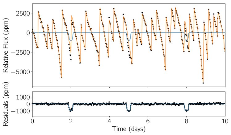
Figure 1: (top): The black points show the raw light curve for the K2 target EPIC 204832142 multiplied by the time series for a simulated transiting planet. The simulated transit model is shown as a blue line. We fit the systematics using the linear model from the everest library (Luger et al., 2016, 2017) and the prediction for the systematics model (Equation 3) is shown as an orange line. (bottom): The same data from the top panel with the systematics model subtracted. The transit model is plotted in blue.

5 Appendix

The marginalized likelihood may be expressed as follows:

$$p({\boldsymbol{y}}|{\boldsymbol{\theta}}) =\frac{1}{|2\pi{\boldsymbol{\Lambda}}|^{\frac{1}{2}}|2\pi{\boldsymbol{C}}|^{\frac{1}{2}}}\int_{-\infty}^{\infty}\exp\left[-\frac{1}{2}z\right]\mathrm{d}{\boldsymbol{w}}$$ (6)

where

$$z ={\boldsymbol{w}}^{\top}{\boldsymbol{\Lambda}}^{-1}{\boldsymbol{w}}+({\boldsymbol{r}}-{\boldsymbol{A}}{\boldsymbol{w}})^{\top}{\boldsymbol{C}}^{-1}({\boldsymbol{r}}-{\boldsymbol{A}}{\boldsymbol{w}})$$ (7)

and ${\boldsymbol{r}}={\boldsymbol{y}}-{\boldsymbol{\mu}}({\boldsymbol{\theta}})$. The integral is easier to evaluate if we complete the square and write:

$$z =({\boldsymbol{w}}-{\boldsymbol{h}})^{\top}{\boldsymbol{\Sigma}}^{-1}({\boldsymbol{w}}-{\boldsymbol{h}})+k\quad,$$ (8)

where, by comparison with Equation (7), it can be shown that

$${\boldsymbol{\Sigma}}^{-1} ={\boldsymbol{\Lambda}}^{-1}+{\boldsymbol{A}}^{\top}{\boldsymbol{C}}^{-1}{\boldsymbol{A}}$$ (9)

$${\boldsymbol{h}} ={\boldsymbol{\Sigma}}{\boldsymbol{A}}^{\top}{\boldsymbol{C}}^{-1}{\boldsymbol{r}}$$ (10)

$$k ={\boldsymbol{r}}^{\top}\left({\boldsymbol{C}}^{-1}-{\boldsymbol{C}}^{-1}{\boldsymbol{A}}{\boldsymbol{\Sigma}}{\boldsymbol{A}}^{\top}{\boldsymbol{C}}^{-1}\right){\boldsymbol{r}}\quad.$$ (11)

We may thus write

$$p({\boldsymbol{y}}|{\boldsymbol{\theta}})=\frac{1}{|2\pi{\boldsymbol{\Lambda}}|^{\frac{1}{2}}|2\pi{\boldsymbol{C}}|^{\frac{1}{2}}}\exp\left[-\frac{k}{2}\right]\int_{-\infty}^{\infty}\exp\left[-\frac{1}{2}({\boldsymbol{w}}-{\boldsymbol{h}})^{\top}{\boldsymbol{\Sigma}}^{-1}({\boldsymbol{w}}-{\boldsymbol{h}})\right]\mathrm{d}{\boldsymbol{w}}\quad.$$ (12)

The integral is that of a Gaussian, which evaluates to $|2\pi{\boldsymbol{\Sigma}}|^{\frac{1}{2}}$. By the Matrix Determinant Lemma and the Woodbury Identity (for example, Woodbury, 1950; Harville, 1997),

$$|{\boldsymbol{\Sigma}}| ={|{\boldsymbol{\Sigma}}^{-1}|}^{-1}=\frac{|{\boldsymbol{\Lambda}}||{\boldsymbol{C}}|}{|{\boldsymbol{C}}+{\boldsymbol{A}}{\boldsymbol{\Lambda}}{\boldsymbol{A}}^{\top}|}$$

$$k ={\boldsymbol{r}}^{\top}\left({\boldsymbol{C}}+{\boldsymbol{A}}{\boldsymbol{\Lambda}}{\boldsymbol{A}}^{\top}\right)^{-1}{\boldsymbol{r}}\quad.$$ (13)

Combining these results, the expression in Equation (12) simplifies to

$$p({\boldsymbol{y}}|{\boldsymbol{\theta}}) =\frac{1}{|2\pi({\boldsymbol{C}}{+}{\boldsymbol{A}}{\boldsymbol{\Lambda}}{\boldsymbol{A}}^{\top})|^{\frac{1}{2}}}\exp\left[{-}\frac{1}{2}\big{(}{\boldsymbol{y}}\,{-}\,{\boldsymbol{\mu}}({\boldsymbol{\theta}})\big{)}^{\top}({\boldsymbol{C}}{+}{\boldsymbol{A}}{\boldsymbol{\Lambda}}{\boldsymbol{A}}^{\top})^{-1}\big{(}{\boldsymbol{y}}\,{-}\,{\boldsymbol{\mu}}({\boldsymbol{\theta}})\big{)}\right].$$ (14)

This is a normal distribution with mean ${\boldsymbol{\mu}}({\boldsymbol{\theta}})$ and covariance ${\boldsymbol{C}}+{\boldsymbol{A}}{\boldsymbol{\Lambda}}{\boldsymbol{A}}^{\top}$:

$$p({\boldsymbol{y}}|{\boldsymbol{\theta}}) =\mathcal{N}({\boldsymbol{y}};{\boldsymbol{\mu}}({\boldsymbol{\theta}}),{\boldsymbol{C}}+{\boldsymbol{A}}{\boldsymbol{\Lambda}}{\boldsymbol{A}}^{\top})\quad.$$ (15)

References

Fergus et al. (2014)
Fergus, R., et al. 2014, ApJ, 794, 161
Harville (1997)
Harville, D. A. 1997, Matrix algebra from a statistician’s perspective, Vol. 1
(Springer)
Luger et al. (2016)
Luger, R., et al. 2016, AJ, 152, 100
Luger et al. (2017)
—. 2017, ArXiv e-prints, arXiv:1702.05488
Ness et al. (2015)
Ness, M., et al. 2015, ApJ, 808, 16
Rasmussen & Williams (2006)
Rasmussen, C. E., & Williams, K. I. 2006, Gaussian Processes for Machine
Learning (MIT Press)
Smith et al. (2012)
Smith, J. C., et al. 2012, PASP, 124, 1000
Tsalmantza & Hogg (2012)
Tsalmantza, P., & Hogg, D. W. 2012, ApJ, 753, 122
Wang et al. (2016)
Wang, D., et al. 2016, PASP, 128, 094503
Wang et al. (2017)
—. 2017, ArXiv, arXiv:1710.02428
Woodbury (1950)
Woodbury, M. A. 1950, Memorandum report, 42, 336