Revisiting CMB constraints on Warm Inflation

Abstract

We revisit the constraints that Planck 2015 temperature, polarization and lensing data impose on the parameters of warm inflation. To this end, we study warm inflation driven by a single scalar field with a quartic self interaction potential in the weak dissipative regime. We analyse the effect of the parameters of warm inflation, namely, the inflaton self coupling $\lambda$ and the inflaton dissipation parameter $Q_{P}$ on the CMB angular power spectrum. We constrain $\lambda$ and $Q_{P}$ for 50 and 60 number of e-foldings with the full Planck 2015 data (TT, TE, EE + lowP and lensing) by performing a Markov-Chain Monte Carlo analysis using the publicly available code CosmoMC and obtain the joint as well as marginalized distributions of those parameters. We present our results in the form of mean and 68 % confidence limits on the parameters and also highlight the degeneracy between $\lambda$ and $Q_{P}$ in our analysis. From this analysis we show how warm inflation parameters can be well constrained using the Planck 2015 data.

1 Introduction

Cosmic inflation [1, 2, 3, 4, 5, 6, 7, 8, 9] is a phase of accelerated expansion in the early history of the Universe during which the energy density of the Universe is dominated by the density of a slowly rolling scalar field, the inflaton. In the simplest models of this inflationary paradigm, it is assumed that the number density of all the particles becomes negligible during inflation due to which slow roll inflation occurs in an almost perfect vacuum state. The inflaton field is coupled to other fields so that it may dissipate its energy after inflation and reheat the universe. However one may consider the possibility that dissipative effects are important not only after but also during the slow-roll phase of inflation. In that case, under appropriate conditions, there is a thermal bath present during the accelerated expansion also, and if the temperature of the bath is greater than the Hubble parameter $H$, then this scenario is known as Warm Inflation [10, 11, 12](see Ref. [13] for a more recent discussion on dissipation during inflation).

Why should one consider warm inflation? Firstly, it is natural to consider inflaton couplings not just during reheating but also during inflation. Furthermore, for some warm inflation models, the eta problem, namely, the presence of large quantum corrections to the inflaton potential that ruins its flatness, is resolved. Also, some potentials that are excluded by Cosmic Microwave Background (CMB) data in the cold inflation scenario are allowed in the warm inflation scenario (though the converse is also true). Models of warm inflation usually require a very large number of fields ($10^{4}-10^{6}$) to be coupled to the inflaton to maintain a thermal bath with $T>H$ [14, 15], which may be unattractive. However recently proposed warm inflation models with the inflaton as a pseudo-Nambu-Goldstone boson require only two additional fields [16, 17].

Given the importance of warm inflation, it is then important to constrain the parameters of warm inflation scenarios using Cosmic Microwave Background (CMB) data just like it is done for various cold inflation scenarios. In this work, we constrain the parameters of warm inflation driven by a quartic potential using complete Planck 2015 data (temperature, polarization and lensing). In particular, we focus on obtaining the marginal and joint probability distributions of the parameters involved in the model by carrying out a full Markov-Chain Monte Carlo analysis using CosmoMC [18], a publicly available code.

A quartic warm inflation model is described by the inflaton’s self coupling $\lambda$ and its dissipation rate to other fields described by the dissipation coefficient $\Upsilon$. In the literature there are usually two forms for this dissipation coefficient, $C_{T}T$ and $C_{\phi}T^{3}/\phi^{2}$. Here we consider only the latter form, which is obtained from inflaton decay to lighter particles mediated by heavier particles ($T>m$) [19, 20, 21] and $C_{\phi}$ is related to the inflaton couplings and the multiplicities of other fields in the model. More generally, $\Upsilon=CT^{c}\phi^{2a}/M_{X}^{2b}$ with $c+2a-2b=1$ [22], where $M_{X}$ is the mass of the intermediate particle. For a model builder, knowing constraints from the data on $\lambda$ and $C_{\phi}$ will be very useful.

The power spectrum for quartic warm inflation depends on $\lambda,C_{\phi}$ and $\phi_{k}$, where the subscript $k$ indicates that quantities are evaluated at the time when the scale $k$ crosses the horizon during inflation. In the literature on warm inflation, the authors have introduced the variable $Q=\Upsilon/(3H)$. The power spectrum for quartic chaotic warm inflation then effectively depends on $\lambda,Q_{k}$ and $N_{k}$, the number of e-foldings of inflation from the end of inflation to the epoch when the scale $k$ crosses the horizon. [Recall that in cold inflation the power spectrum can be made to be effectively dependent on $\lambda$ and $N_{k}$ (see, for example, Eq. (8.71) of Ref. [23] for quartic chaotic inflation).]

For cold inflation, the normalisation of the power spectrum at the pivot scale $k_{P}$ fixes the value of $\lambda$, for a fixed $N_{P}$, where $P$ indicates that quantities are evaluated at the time when the pivot scale $k_{P}$ crosses the horizon during inflation. We find that in warm inflation too fixing the normalisation at the pivot scale fixes the value of $\lambda$ for fixed $N_{P}$ and a particular value of $Q_{P}$. We find that for the scales of cosmological interest the power spectrum is close to power law, and we study the dependence of the primordial power spectrum on the parameters of the model. We then study the angular power spectrum using the publicly available code CAMB [37] and finally constrain the parameters of the quartic warm inflation model using CosmoMC. In our analysis, we fix $N_{P}$ to be either 50 or 60.

We begin by summarizing the known results about the primordial power spectrum in warm inflation. We then express the primordial power spectrum for the warm inflation model with a quartic potential as a function of $\lambda,C_{\phi}$ and $Q_{P}$, and then eventually in terms of $\lambda,Q_{P}$ and $N_{P}$. We discuss features of the power spectrum and correlations between parameters of the model. Thereafter we present our Monte-Carlo Markov Chain analysis using CosmoMC for which we use the full Planck 2015 data (high-l TT,TE, TE + low-l polarization + lensing) for our analysis. We explain how we constrain the parameters of quartic warm inflation and finally show the obtained joint and marginal probability distributions of $\lambda$ and $Q_{P}$. We provide the mean and standard deviation for these parameters and highlight the degeneracy between the parameters.

2 Evolution equations in warm inflation

For the inflaton $\phi$ interacting with other fields the evolution is governed by

$$\ddot{\phi}-\nabla^{2}\phi+3H\dot{\phi}+\Upsilon\dot{\phi}+V^{\prime}=(2\Upsilon T)^{\frac{1}{2}}\xi(x,t)\;,$$ (2.1)

where, $H$ is the Hubble parameter during inflation, the overdots are derivatives w.r.t. cosmic time, prime indicates the derivative w.r.t. $\phi$, $\Upsilon$ is the inflaton dissipation rate and $\xi$ represents stochastic fluctuations due to interactions of $\phi$ with other species. The stochastic r.h.s and the dissipation rate on the l.h.s are related through the fluctuation-dissipation theorem [25, 24, 22]. For the background homogeneous field $\phi(t)$, and a zero mean for $\xi(t)$

$$\ddot{\phi}+3H\dot{\phi}+\Upsilon\dot{\phi}+V^{\prime}=0\;.$$ (2.2)

Recall that for a damped harmonic oscillator, $\ddot{x}+2b\dot{x}+\omega^{2}x=0$, and the friction term, i.e. $2b\dot{x}$, causes dissipation and non-conservation of energy. Moreover, the rate of loss of energy is given by $dE/dt=-b\dot{x}^{2}$. Similarly, during warm inflation, for the scalar field we have [26]

$$\dot{\rho}_{\phi}+3H(\rho_{\phi}+p_{\phi})=-\Upsilon{\dot{\phi}}^{2},$$ (2.3)

where $\Upsilon{\dot{\phi}}^{2}$ is the rate at which the inflaton loses energy. Dissipation causes radiation to be produced and the radiation energy density $\rho_{r}$ evolves as

$$\dot{\rho}_{r}+4H\rho_{r}=\Upsilon{\dot{\phi}}^{2}~{}.$$ (2.4)

Assuming the radiation thermalises quickly, the radiation energy density and temperature are related by

$$\rho_{r}=(\pi^{2}/30)g_{*}T^{4},$$ (2.5)

where, $T$ is the temperature of the radiation bath and $g_{*}$ is the number of relativistic degrees of freedom during warm inflation. The notion of thermal equilibrium and a temperature is only valid for $T_{k}>H_{k}$, as the Hubble radius $H_{k}^{-1}$ is then greater than the thermal de Broglie wavelength $\sim T_{k}^{-1}$ [27]. This then gives a lower bound on $Q_{P}$, as we discuss later.

The various different realizations of warm inflation lead to different dependences of $\Upsilon$ on the temperature. Here we focus on the models of warm inflation in which the inflaton is coupled only indirectly to light fields $(m<T)$ through heavy mediator fields $(m>T)$. (Direct coupling of light fields to the inflaton gives large thermal corrections to the potential thereby spoiling its flatness and effectively leading to too few e-foldings of inflation [28, 29].) Then one finds that [19, 20, 21]

$$\Upsilon(\phi,T)=C_{\phi}\frac{T^{3}}{\phi^{2}}\;,$$ (2.6)

where $C_{\phi}$ is a dimensionless constant. Typically, in supersymmetric models such as the ones considered in Ref. [21, 27] one gets

$$C_{\phi}=\frac{h^{2}}{16\pi}N_{X}N_{Y}\;,$$ (2.7)

where $N_{X}$ and $N_{Y}$ are the number of heavy mediator fields and light fields respectively and $h$ is a Yukawa coupling. Note that for a small effective Yukawa coupling of $h\sqrt{N}_{Y}$ there can be a large contribution to $\Upsilon$ from dissipation to on shell heavy mediator particles, that later decay to Y particles, due to a narrow resonance that overcomes the Boltzmann suppression [21].

In the slow roll approximation, one can ignore the $\ddot{\phi}$ term, and the background field evolution equation gives

$$\dot{\phi}\approx\frac{-V^{\prime}(\phi)}{3H(1+Q)}\,,$$ (2.8)

where $Q$ is defined by

$$Q=\frac{\Upsilon(\phi,T)}{3H(t)}.$$ (2.9)

Similarly, ignoring $\dot{\phi}^{2}$ as compared to $V(\phi)$, and the sub-dominant $\rho_{r}$, Einstein’s equation implies that

$$H^{2}=\frac{8\pi}{3}\frac{V(\phi)}{M_{\rm Pl}^{2}}\;,$$ (2.10)

where $M_{\rm Pl}=1/{\sqrt{G}}=1.2\times 10^{19}$ GeV is the Planck mass. The slow roll parameters for warm inflation are defined as

$$\epsilon_{\phi}=\frac{M_{Pl}^{2}}{16\pi}\,\left(\frac{V_{,\phi}}{V}\right)^{2},\quad\eta_{\phi}=\frac{M_{Pl}^{2}}{8\pi}\,\frac{V_{,\phi\phi}}{V},\quad\beta_{\Upsilon}=\frac{M_{Pl}^{2}}{8\pi}\,\left(\frac{\Gamma_{,\phi}\,V_{,\phi}}{\Gamma\,V}\right)\,.$$ (2.11)

In the literature, one also defines the Hubble flow function [30]

$$\epsilon_{1}=\frac{d\ln(H_{P}/H)}{dN}=-\frac{\dot{H}}{H^{2}}\;.$$ (2.12)

The slow roll parameters and the Hubble flow function are evaluated at the pivot scale. Setting $\dot{H}=H_{,\phi}\dot{\phi}$ it is easy to verify that

$$\epsilon_{1}=\frac{\epsilon_{\phi}}{1+Q}=\frac{1}{1+Q}\frac{M_{\rm Pl}^{2}}{16\pi}\left(\frac{V^{\prime}}{V}\right)^{2}.$$ (2.13)

The slow roll conditions needed for the inflationary phase are [31]

$$\epsilon_{\phi}\ll 1+Q,\quad|\eta_{\phi}|\ll 1+Q,\quad|\beta_{\Upsilon}|\ll 1+Q\,.$$ (2.14)

In warm inflation one presumes that $\dot{\rho}_{r}\approx 0$ and the temperature of the Universe is approximately unchanged. Then

$$\rho_{r}\approx\frac{3}{4}Q{\dot{\phi}}^{2}\,.$$ (2.15)

Figures (1) and (5) show how $\rho_{r}$ and $T$ vary with time during warm inflation. $\dot{\rho}_{r}\approx 0$ is valid when modes of cosmological interest cross the horizon during inflation, but it seems to be only approximately true for the entire duration of inflation. However $\dot{\rho}_{r}$ is small compared to the other terms in Eq. (2.4) throughout inflation and hence the approximation is valid.

3 Warm inflation model with a quartic potential

We consider a warm inflation model with a quartic potential

$$V(\phi)=\lambda\phi^{4}\,$$ (3.1)

and a dissipation coefficient $\Upsilon=C_{\phi}\frac{T^{3}}{\phi^{2}}$. Then

$$Q=\frac{\Upsilon}{3H}=\frac{C_{\phi}}{3H}\frac{T^{3}}{\phi^{2}}\;.$$ (3.2)

For a quartic potential, we get

$$H^{2}=\frac{8\pi}{3}\frac{\lambda\phi^{4}}{M_{\rm Pl}^{2}}$$ (3.3)

and the Hubble flow function

$$\epsilon_{1}=\frac{1}{1+Q}\frac{1}{16\pi}\left(\frac{M_{\rm Pl}}{\phi}\right)^{2}.$$ (3.4)

It is easy to verify that $\epsilon_{\phi}=\frac{2}{3}\eta_{\phi}=-\beta_{\Upsilon}$.

3.1 The primordial power spectrum

The scalar primordial power spectrum is given in Ref. [27] (based on Refs. [10, 33, 12, 32, 22]) as

$$P_{\mathcal{R}}(k)=\left(\frac{H_{k}^{2}}{2\pi\dot{\phi}_{k}}\right)^{2}\left[1+2n_{k}+\left(\frac{T_{k}}{H_{k}}\right)\frac{2\sqrt{3}\pi Q_{k}}{\sqrt{3+4\pi Q_{k}}}\right]~{},$$ (3.5)

where $n(k)$ is the distribution of quanta of inflaton fluctuations $\delta\phi$ and the subscript $k$ refers to the time when a $k$ mode leaves the Hubble radius during inflation. Treating the inflaton field and the radiation as coupled fluids, it has been argued that perturbations in the radiation, because of inhomogeneous dissipation, can lead to a growing mode in the inflaton perturbations which causes an enhancement in the primordial power spectrum in terms of a multiplicative factor whose form depends on the form of $\Upsilon$ [34, 17]. For a cubic dissipation coefficient, it is obtained numerically in Ref. [42] as $G_{{\rm cubic}}(Q_{P})=1+4.981\ Q_{P}^{1.946}+0.127\ Q_{P}^{4.330}$. As our analysis is done for the weak dissipation regime, $10^{-5}<Q_{P}<10^{-1}$, we can neglect it, as it is approximately 1 for the whole range of $Q_{P}$ of interest to us. (For large dissipation, $Q_{P}\gg 1$, it was argued that inflaton perturbations can be sufficiently enhanced to make them incompatible with observations [25], but subsequently it was shown that shear viscosity in the non-equilibrium radiation damps the radiation perturbations and hence the enhancement of the inflaton perturbations.) The tensor power spectrum is given by the same expression as in cold inflation, namely,

$$P_{T}(k)=\frac{16}{\pi}\left(\frac{H_{k}}{M_{\rm Pl}}\right)^{2}\;.$$ (3.6)

We wish to express the scalar and tensor power spectra as functions of $k$. To this end, we look at the each term appearing in Eq. (3.5) individually:

• Prefactor: Using Eqs. (2.8) and (3.3)

  $$\frac{H_{k}^{2}}{2\pi\dot{\phi}_{k}}=\sqrt{\frac{8\pi}{3}}\sqrt{\lambda}\left(\frac{\phi_{k}}{M_{\rm Pl}}\right)^{3}(1+Q_{k})\,.$$ (3.7)

• $T/H$ term: Using the expression for $\rho_{r}(T)$ in Eq. (2.15), and Eqs. (2.8), (3.1) and (3.3) we get

  $$T_{k}=\left(\frac{15}{\pi^{3}g_{*}}\frac{Q_{k}}{(1+Q_{k})^{2}}\lambda\,\phi_{k}^{2}M_{\rm Pl}^{2}\right)^{\frac{1}{4}}\;.$$ (3.8)

  Furthermore from Eq. (3.3) we obtain

  $$\frac{T_{k}}{H_{k}}=\left(\frac{15}{\pi^{3}g_{*}}\right)^{\frac{1}{4}}\sqrt{\frac{3}{8\pi}}\lambda^{-\frac{1}{4}}\frac{Q_{k}^{\frac{1}{4}}}{(1+Q_{k})^{\frac{1}{2}}}\left(\frac{\phi_{k}}{M_{\rm Pl}}\right)^{-\frac{3}{2}}\;.$$ (3.9)

• Occupation number: We take the inflaton distribution, $n_{k}$, to be represented by a Bose-Einstein distribution,

  $$n_{k}=\frac{1}{\exp(\frac{k/a_{k}}{T_{k}})-1}$$ (3.10)

  where $a$ is the scale factor and $T$ represents the physical temperature. Then the first two terms in the square bracket of Eq. (3.5) become

  $$1+2n_{k}=\coth\frac{H_{k}}{2T_{k}}\,,$$ (3.11)

  with $H_{k}/T_{k}$ obtained from Eq. (3.9). If $n_{k}=0$ then

  $$1+2n_{k}\rightarrow 1\,.$$ (3.12)

  We discuss the importance of the $\coth$ term in Sec. §5.2.

The above discussion implies that the scalar power spectrum in Eq. (3.5) depends on $\lambda$, $Q_{k}$ and $\phi_{k}$. Furthermore, using the slow roll equations, Eqs. (2.8) and (2.15), and Eq. (2.6) for $T$, one can express $Q_{k}$ as a function of $\phi_{k}$. This can then be inverted to give $\phi_{k}$ in terms of $Q_{k}$, as in Eq. (21) of Ref. [35], as

$$\left(\frac{\phi_{k}}{M_{\rm Pl}}\right)=\sqrt{\frac{1}{8\pi}}\left(\frac{64C_{\phi}^{4}\lambda}{9C_{R}^{3}}\frac{1}{Q_{k}(1+Q_{k})^{6}}\right)^{\frac{1}{10}}~{},$$ (3.13)

where $C_{R}=(\pi^{2}/30)g_{*}$.

3.2 Obtaining the dissipation parameter $Q_{k}$

In order to obtain the $k$ dependence of the scalar power spectrum, we need to find the $k$ dependence of $Q_{k}$. From Eq. (13) of Ref. [27] (based on Ref. [35]) we have

$$\frac{dQ}{dN}=-\frac{1}{C_{1}}\frac{Q^{6/5}(1+Q)^{6/5}}{1+7Q}~{},$$ (3.14)

where $N=\ln(a_{e}/a)$ is the number of e-foldings of inflation from the end of inflation, and

$$C_{1}=\frac{1}{40}\left(\frac{64C_{\phi}^{4}\lambda}{9C_{R}^{3}}\right)^{\frac{1}{5}}~{}.$$ (3.15)

In order to find the $k$ dependence, it is useful to define $x=\ln(k/k_{P})$. Then,

$$\frac{dQ}{dx}=\frac{dQ}{dN}\frac{dN}{dx}\;.$$ (3.16)

Since $N=\ln(a_{e}/a)$ and $a=k/H$, $dN/dx=-1+H^{-1}dH/dx=-1+H^{-1}(dH/dN)\,(dN/dx)$. Then using $\epsilon_{1}=H^{-1}dH/dN$, we get

$$\frac{dN}{dx}=-\frac{1}{1-\epsilon_{1}}\,.$$ (3.17)

Therefore

$$\frac{dQ}{dx}=\frac{1}{[1-\epsilon_{1}]}\frac{1}{C_{1}}\frac{Q^{6/5}(1+Q)^{6/5}}{1+7Q}\;.$$ (3.18)

One integrates the above equation from the time when $k^{th}$ mode leaves the horizon till when the pivot scale crosses the horizon to get a relation between $Q_{k}$ and $k$ in the form of a transcendental equation as

$$G(Q_{k})-G(Q_{p})=x\,,$$ (3.19)

where

$$G(Q) =\frac{C_{1}}{12Q^{1/5}(1+Q)^{6/5}}\left[-32\left(\frac{10125\pi^{6}Q(1+Q)^{6}}{C^{4}_{\phi}\lambda}\right)^{1/5}\ln\left(Q(1+Q)^{6}\right)\right.$$

$$+\left.15(1+Q)\left(-4+20Q-15Q(1+Q)\,_{2}F_{1}\left(1,\frac{8}{5},\frac{9}{5},-Q\right)\right)\right]$$ (3.20)

and ${}_{2}F_{1}(a,b,c,z)$ is the Hypergeometric function.

Combining Eqs. (3.19) and (3.20) with the expressions in Sec. §3.1 we can express the power spectrum $P_{\mathcal{R}}$ as a function of $k$, and the parameters $\lambda,C_{\phi}$ and $Q_{P}$.

3.3 Duration of inflation

We have to ensure that the parameters we choose for the power spectrum correspond to a scenario that gives sufficient e-foldings of inflation. Applying the condition that inflation lasts for $N_{P}$ e-foldings after the pivot scale crosses the horizon during inflation provides a relation between the parameters $\lambda$ and $C_{\phi}$. Integrating Eq. (3.14) from the time when $k^{th}$ mode leaves the horizon till when the pivot scale crosses the horizon we get

$$N_{k}-N_{P}=C_{1}[F(Q_{P})-F(Q_{k})]\,,$$ (3.21)

where $C_{1}$ is as given in Eq. (3.15) and

$$F(Q)=\frac{5}{4Q^{\frac{1}{5}}(1+Q)}\left[4(1+Q)^{\frac{4}{5}}(-1+5Q)-15Q(1+Q)\cdot~{}_{2}F_{1}\left(\frac{1}{5},\frac{4}{5},\frac{9}{5},-Q\right)\,\right]\,,$$ (3.22)

where again ${}_{2}F_{1}(a,b,c,z)$ is the Hypergeometric function.

Let us consider the mode which crosses the Hubble radius at the end of inflation. For such a mode $N_{k}=0$ and Eq. (3.21) implies that

$$N_{P}=C_{1}[F(Q_{e})-F(Q_{P})]\,.$$ (3.23)

We can obtain $Q_{e}$ by setting the second potential slow roll parameter $\eta_{\phi}$ to $1+Q_{e}$, i.e.

$$\eta_{e}=\frac{3}{2\pi}\frac{M_{\rm Pl}^{2}}{\phi_{e}^{2}}=1+Q_{e}\,.$$ (3.24)

For the model under consideration, warm inflation ends because the slow roll conditions fail, and not because $\rho_{r}$ overtakes $\rho_{\phi}$, as seen in Figure (1), where $\rho_{\phi e}\sim 3\rho_{re}$. (Since, as shown earlier, $\eta_{\phi}$ is the largest slow roll parameter it is sufficient to verify the breakdown of the slow roll condition with $\eta_{\phi}$.) Expressing $\phi_{e}$ in terms of $Q_{e}$ using Eq. (3.13) we get

$$Q_{e}^{2}+Q_{e}-\left(\frac{64C_{\phi}^{4}\lambda}{9C_{R}^{3}}\right)\frac{1}{12^{5}}=0\,,$$ (3.25)

whose positive solution is

$$Q_{e}=\frac{-1+\sqrt{1+4\left(\frac{64C_{\phi}^{4}\lambda}{9C_{R}^{3}}\right)\frac{1}{12^{5}}}}{2}\,.$$ (3.26)

Notice that $Q_{e}$ depends on $\lambda C_{\phi}^{4}$.

Using the expressions for $C_{1}$ (Eq. (3.15)) and $Q_{e}$ (Eq. (3.26)) in Eq. (3.23), we get a value for $\lambda C_{\phi}^{4}$ for a given value of $N_{P}$ and $Q_{P}$ which we can use to express $C_{\phi}$ in terms of $\lambda$. Using this in $P_{\mathcal{R}}(k)$ the parameters defining the power spectrum are now $\lambda,Q_{P}$ and $N_{P}$. Similarly one can obtain the tensor power spectrum $P_{T}(k)$ in terms of these parameters. By choosing the value of $N_{P}$ appropriately to be, say 50 or 60, we can ensure that we have a sufficient duration of inflation.

Thus, the above implies that it is the values of $\lambda,Q_{P}$ and $N_{P}$ that need to be constrained from the CMB observational data. Therefore in our CosmoMC code we vary the parameters $\lambda$ and $Q_{P}$ while keeping $N_{P}$ fixed for a particular run.

As an aside we note that,

$$N_{k} = \ln\frac{a_{e}}{a_{k}}=\ln\frac{a_{e}}{a_{P}}+\ln\frac{a_{P}}{a_{k}}$$ (3.27)

$$= N_{P}+\ln\left(\frac{k_{P}}{k}\frac{H_{k}}{H_{P}}\right)$$ (3.28)

$$= N_{P}+\ln\frac{k_{P}}{k}+\ln\frac{\phi^{2}_{k}}{\phi^{2}_{P}}\,,$$ (3.29)

which, using Eq. (3.13), gives

$$N_{k}-N_{P}=-\ln\frac{k}{k_{P}}+\ln\left[\frac{Q_{P}(1+Q_{P})^{6}}{Q_{k}(1+Q_{k})^{6}}\right]^{\frac{1}{5}}\;.$$ (3.30)

Combining Eqs. (3.21) and (3.30) then gives us $Q_{k}$ as a function of $\ln(k/k_{P})$, for a given $Q_{P}$ and $N_{P}$. We have numerically confirmed that this agrees with the $Q_{k}(x)$ that we obtain from Eqs. (3.19) and (3.20). In our numerical code we use Eqs. (3.19) and (3.20).

4 Primary analysis using the primordial power spectrum and its normalisation

In the last section we argued that the primordial power spectrum is completely determined by the values of the three parameters $N_{P}$, $Q_{P}$ and $\lambda$. These will be the parameters we vary when we perform a detailed data analysis with CosmoMC. But before presenting those results, we shall study using Mathematica the power spectrum and understand how these parameters determine various features of the quartic model under consideration. For this section we also impose the normalisation of the power spectrum as $P_{\mathcal{R}}(k_{P})\equiv A_{s}=2.2\times 10^{-9}$. For any given value of $Q_{P}$ and $N_{P}$ this constraint then fixes $\lambda$. To appreciate how parameters change during warm inflation we also plot the homogeneous inflaton field $\phi$, $Q_{k}$ and the energy density of $\phi$ and the radiation as a function of the number of efoldings of inflation in Figure (1).

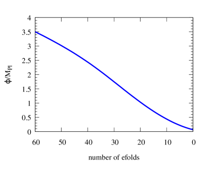
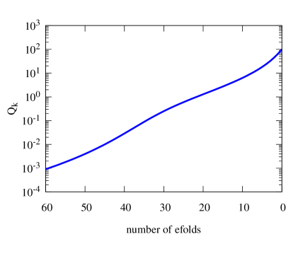
Figure 1: The behaviour of the homogeneous inflaton field $\phi$, $Q_{k}$, and the energy density in $\phi$ and radiation is shown as a function of the number of efoldings $N$. Note that as $Q$ crosses 1 during inflation the model transits from weak dissipation to strong dissipation. For our model $\rho_{\phi}$ is larger than $\rho_{r}$ till when the slow roll conditions fail and the latter therefore determines when inflation ends. Consequently the Universe will also go through a phase of reheating after inflation. All plots correspond to $N_{P}=50$ and fixed $A_{s}$, and $Q_{P}=10^{-2.4}$.

4.1 Spectral index

We first plot the power spectrum for different values of $Q_{P}$ while keeping $N_{P}$ fixed at $50$ and $A_{s}$ fixed as above. This is shown in Figure (2), along with the standard power law power spectrum with $n_{s}$ equal to the mean value of $0.9653$ obtained by the Planck collaboration with TT, TE, EE + low P + lensing 2015 data [36]. The different plots for warm inflation correspond to different values of $\lambda$, chosen appropriately to give the correct normalisation $A_{s}$. It is noteworthy that as we decrease $Q_{P}$ from $10^{-1}$ to $10^{-2.2}$, the slope of the power spectrum decreases, and then increases as we further decrease $Q_{P}$ to $10^{-5}$. This behaviour is best understood by studying the dependence of $n_{s}$ on $Q_{P}$ in Figure (3). It is also worth noting from Figure (3) that for none of the values of $Q_{P}$ in the range we shall study will the power spectrum fall on top of the standard power law spectrum (the solid line in Figure (2)).

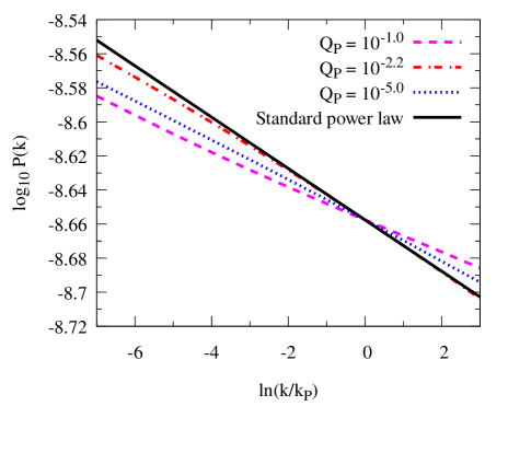
Figure 2: The primordial power spectrum, ${\rm{log}}_{10}P_{\mathcal{R}}(k)$ vs $\ln(k/kp)$ is shown for different values of $Q_{P}$ for $N_{P}=50$ and $A_{s}$ fixed. The coupling $\lambda$ is different for different values of $Q_{P}$. The standard power law with $n_{s}=0.9653$ is also shown as a solid (black) line.

One can determine the scalar spectral index as

$$\left.n_{s}-1\right.\equiv\left.\frac{d\ln P_{\mathcal{R}}(k)}{d\ln(k/k_{P})}\right\rvert_{k=k_{P}}=\left.\frac{d\ln P_{\mathcal{R}}}{dQ_{k}}\frac{dQ_{k}}{d\ln(k/k_{P})}\right\rvert_{k=k_{P}}\;.$$ (4.1)

We obtain the first derivative by expressing $P_{\mathcal{R}}(k)$ in terms of $Q_{k}$ using Eqs. (3.5,3.7,3.9,3.11) and (3.13) and then by taking the derivative w.r.t. $Q_{k}$. $\frac{dQ_{k}}{d\ln(k/k_{P})}$ is given in Eq. (3.18). Then the scalar spectral index can be written as

$$n_{s}= 1-\frac{3\epsilon_{1}}{1-\epsilon_{1}}+\frac{10\epsilon_{1}\ Q_{P}}{(1+7Q_{P})(1-\epsilon_{1})}$$

$$+\frac{1}{(1-\epsilon_{1})}\frac{4n_{P}\epsilon_{1}}{1+2n_{P}+\delta}\left(\frac{e^{H_{P}/T_{P}}}{e^{H_{P}/T_{P}}-1}\frac{H_{P}}{T_{P}}\right)\left(\frac{1+2Q_{P}}{1+7Q_{P}}\right)$$

$$+\frac{1}{(1-\epsilon_{1})}\frac{\delta\epsilon_{1}}{(1+7Q_{P})}\frac{1}{1+2n_{P}+\delta}\left[2+4Q_{p}+5(1+Q_{P})\left(\frac{3+2\pi Q_{P}}{3+4\pi Q_{P}}\right)\right]\,,$$ (4.2)

where $n_{P}=n(k_{P})_{k_{P}}$ and we define $\delta=\frac{2\sqrt{3}\pi Q_{P}}{\sqrt{3+4\pi Q_{P}}}\frac{T_{P}}{H_{P}}$.

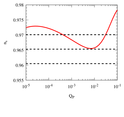
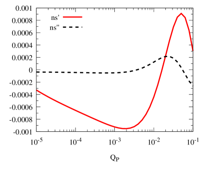
Figure 3: The behaviour of the scalar spectral index, $n_{s}$, as we change $Q_{P}$ for $N_{P}=50$ and $A_{s}$ fixed is shown by the solid curve in the first panel. The three horizontal dashed lines show the mean value and 68 $\%$ CL limits on $n_{s}$ for Planck 2015 TT, TE, EE + low P + lensing data for power law primordial power spectrum $(0.9653\pm 0.0048)$ [36]. Note the non-monotonic behaviour of $n_{s}$. The running of the spectral index $n_{s}^{\prime}\equiv dn_{s}/d(\ln k)$ and the running of the running $n_{s}^{\prime\prime}\equiv d^{2}n_{s}/d(\ln k)^{2}$ as a function of $Q_{P}$ are shown in the second panel for $N_{P}=50$.

The behaviour of $n_{s}$ as we change $Q_{P}$ is shown in Figure (3) which explains the changes in the slope of the power spectrum seen in Figure (2). Note that the value of $n_{s}$ that corresponds to the mean value of $Q_{P}$ of $10^{-2.4}$, obtained by us using CosmoMC, is 0.9659 which differs slightly from the mean value of $n_{s}$ of 0.9653. We also show the running of the spectral index at the pivot scale, and the running of the running, as we vary $Q_{P}$ in the right panel of Figure (3) where we plot $dn_{s}/d(\ln k)$ and $d^{2}n_{s}/d(\ln k)^{2}$ as a function of $Q_{P}$ for $N_{P}$ fixed at $50$. The extremely weak running justifies our use in Figure (3) of the allowed band of $n_{s}$ values from the Planck collaboration for fixed $n_{s}$ without running.

4.2 Coupling parameters $\lambda$ and $C_{\phi}$ as a function of $Q_{P}$

As discussed in Sec. §3.3, $N_{P}$ and $Q_{P}$ determine the value of $\lambda C_{\phi}^{4}$. For $N_{P}=50$, we vary $Q_{P}$ and obtain log${}_{10}\lambda C_{\phi}^{4}$ against $Q_{P}$, as shown in Figure (4). Fitting the log-log plots to a straight line, we get $\lambda{\rm C}_{\phi}^{4}=Q_{P}^{0.60}\times 10^{15.45}$. Imposing the normalisation $A_{s}$ of the power spectrum fixes the value of $\lambda$, as mentioned above, and we obtain $\lambda$ and $C_{\phi}$ as functions of $Q_{P}$ in the other panels in Figure (4). The corresponding fitting functions are $C_{\phi}=Q_{P}^{0.17}\times 10^{7.35}$ and $\lambda=Q_{P}^{-0.10}\times 10^{-14.0}$. This then implies $\lambda\sim C_{\phi}^{-0.57}$.

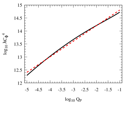
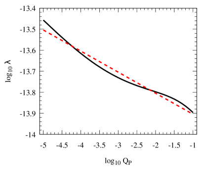
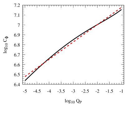
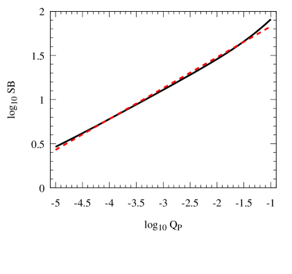
Figure 4: The first panel shows $\lambda{\rm C}_{\phi}^{4}$ as a function of $Q_{P}$ for $N_{P}=50$. The next two panels show $\lambda$ and $C_{\phi}$ as functions of $Q_{P}$ for $N_{P}=50$ and $A_{s}=2.2\times 10^{-9}$. The last panel shows the square bracket in Eq. (3.5) as a function of $Q_{P}$. In all the plots, the black solid curves correspond to the numerical values of the corresponding quantity and the red dashed curves are straight line fits to the log-log plots. For the first panel the fitting function is $\lambda{\rm C}_{\phi}^{4}=Q_{P}^{0.60}\times 10^{15.45}$, for the next two plots they are $C_{\phi}=Q_{P}^{0.17}\times 10^{7.35}$ and $\lambda=Q_{P}^{-0.10}\times 10^{-14.0}$, and for the final plot $SB=Q_{P}^{0.35}\times 10^{2.18}$.

The correlation between $C_{\phi}$ and $Q_{P}$ tells us how the observational limits on $Q_{P}$, the decay width of the inflaton in units of thrice the Hubble parameter can help us estimate $C_{\phi}$. As one can see from Eq. (2.7), $C_{\phi}$ is a function of the Yukawa coupling $h$ and the number of mediators and light fields. As mentioned earlier, in the weak dissipation regime, the mean value of $Q_{P}$ that we obtain using CMB observations is of the order of $10^{-2.4}$. The plot of $C_{\phi}$ vs $Q_{P}$ in Figure (4) then indicates that the corresponding value of $C_{\phi}$ is of the order of $8.8\times 10^{6}$. For values of the Yukawa coupling in the regime of validity of perturbative calculations, this implies that $N_{X}N_{Y}$ is of order a 100 million. Thus, this implementation of warm inflation in which the inflaton couples to light degrees of freedom forming radiation through heavy mediator fields requires the existence of order 100 million fields in the corresponding microscopic theory. This requirement of a large value of $C_{\phi}$, or a large number of fields, has been pointed out in Ref. [14, 26, 27].

4.3 Thermal equilibrium and a lower bound on $Q_{P}$

As mentioned earlier, the temperature is defined only for $T_{k}>H_{k}$. In Figure (5), we plot $T_{k}/H_{k}$ as a function of the number of e-foldings $N$ for different values of $Q_{P}$, and $N_{P}=50$ and fixed $A_{s}$. We find that $T_{k}>H_{k}$ holds for $Q_{P}>10^{-5.0}$. One also notices that $T_{k}/H_{k}$ increases with time till the end of inflation. We also plot $T_{k}$ as a function of $N$. (We mention in passing that the relation between $Q_{P}$ and $T/H$ in Sec. 4 of Ref. [27] has a typographical error.)

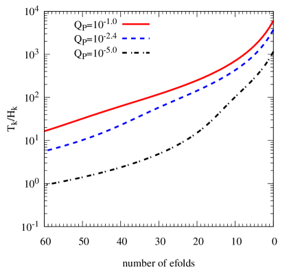
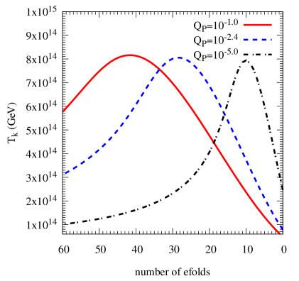
Figure 5: Plots showing $T_{k}/H_{k}$ vs $\ln(k/k_{P})$ and $T_{k}$ vs $\ln(k/k_{P})$ for different values of $Q_{P}$. Note that $T>H$ during inflation is valid only for $Q_{P}>10^{-5}$.

4.4 Correlation between $\lambda$ and $Q_{P}$

We note that for $Q_{P}\ll 1$ sec. §3.1 implies that

$$A_{s}=P_{\cal R}(k_{P}) \sim\lambda\left(\frac{\phi_{P}}{M_{\rm Pl}}\right)^{6}SB\;,$$ (4.3)

$$\sim\lambda\left(\frac{\lambda C_{\phi}^{4}}{Q_{P}}\right)^{\frac{6}{10}}SB\,,$$ (4.4)

where $SB$ refers to the square bracket in Eq. (3.5). The dependence of $\lambda C_{\phi}^{4}$ on $Q_{P}$ is shown in Figure (4). For $N_{P}=50$ and fixed $A_{s}$ we find how $SB$ varies with $Q_{P}$, and this is also shown in Figure (4). Numerical fitting tells us that

$$\lambda C_{\phi}^{4} \sim Q_{P}^{0.60}\;,$$ (4.5)

$$SB \sim Q_{P}^{0.35}\;,$$ (4.6)

and so

$$P_{\cal R}(k_{P}) \sim\lambda\left(\frac{Q_{P}^{0.60}}{Q_{P}}\right)^{\frac{6}{10}}Q_{P}^{0.35}\;,$$

$$\sim\lambda Q_{P}^{0.11}\;,$$ (4.7)

which implies $\lambda\sim Q_{P}^{-0.11}$. (The factorisation of the r.h.s. of Eq. (4.7) into powers of $\lambda$ and $Q_{P}$ is not unique. For example, $SB$ contains $T_{P}/H_{P}$ which has a factor of $\lambda^{-\frac{1}{4}}$. One could try to extract it out explicitly or subsume it in the behaviour of $SB$ as a function of $Q_{P}$, as we have done. Either way, the relation between $\lambda$ and $Q_{P}$ will be the same and as obtained here.)

In Sec. §4.2 we had discussed the relation between $\lambda$ and $Q_{P}$ for fixed $A_{s}$ and $N_{P}$ and found it to be $\lambda=Q_{P}^{-0.10}\times 10^{-14.0}$. Obviously, the fitting function between $\lambda$ and $Q_{P}$ must be the same no matter how it is found, and we find that the $\lambda-Q_{P}$ relations found earlier and in this subsection are mutually consistent, confirming our analysis. Thus, we expect that when we perform the CosmoMC analysis, we should obtain for the joint distribution of $\lambda$ and $Q_{P}$ a correlation between the two characterised by $\lambda\sim Q_{P}^{-0.1}$ for $N_{P}=50$. Repeating the above analysis for $N_{P}=60$ also gives $\lambda\sim Q_{P}^{-0.1}$ and we expect CosmoMC to give a similar result.

5 Analysis of the effects of warm inflation parameters on the CMB angular power spectrum

5.1 $\lambda$ and $Q_{P}$

In Figure (6) we plot the $TT$ angular power spectrum of CMB for fixed $\lambda$ while varying $Q_{P}$, and for fixed $Q_{P}$ while varying $\lambda$, respectively keeping $N_{P}=50$ fixed. We obtain the plots using CAMB. We see that the angular power spectrum is sensitive to even a slight variation in $\lambda$. However it varies considerably only with order of magnitude changes in $Q_{P}$. This behaviour is also suggested by Eq. (4.7).

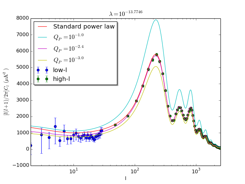
Figure 6: The plot on the left shows the TT angular power spectrum of the CMB for various values of $Q_{P}$, for $\lambda$ fixed at $10^{-13.7746}$ and $N_{P}$ fixed at $50$. The plot on the right shows the TT angular power spectrum of CMB for various values of $\lambda$, for $Q_{P}$ fixed at $10^{-2.4}$ and $N_{P}=50$. For both plots, the best fit corresponds to $Q_{P}=10^{-2.4}$ and $\lambda=10^{-13.7746}$, which overlaps with the $C_{\ell}$’s obtained with the standard power law spectrum with $n_{s}=0.96$. In the plots, low $\ell$ refers to the range $\ell=2-49$ while high $\ell$ refers to the range $\ell=50-2500$ (see Ref. [38] for details).

5.2 Effect of the coth term, and a comparison with cold inflation

A Bose-Einstein distribution for inflatons has been considered in the context of cold inflation too with a similar $\coth[H_{k}/(2T_{k})]$ term [39]. In that case, it is presumed that the inflaton was in thermal equilibrium at some early time prior to inflation, possibly at the Planck time, and subsequently its interactions froze out. Therefore one has a frozen distribution of inflatons at the beginning of inflation. Since this distribution dilutes with the expansion of the Universe, and hence during inflation, the effect of the thermal distribution is larger for larger scales. In fact, it enhances power on larger scales and if the power spectrum is pivoted at a standard pivot scale then, as seen in Fig. (1) of Ref. [39], there is excess power on large scales which requires inflation to last 7-32 more e-foldings than the standard requirement for GUT scale to electoweak scale inflation so as to dilute the effect of the inflaton distribution.

For warm inflation where one considers a thermal distribution of inflatons the distribution is replenished by dissipation and the temperature is approximately constant when cosmologically relevant $k$ modes leave the horizon. For $N_{P}=50$ and fixed $A_{s}$, and $Q_{P}=10^{-2.4}$, we find that $\coth[H_{k}/(2T_{k})]$ varies from 13 to 26 as $x$ varies from $-7$ to $3$. The ratio of the square bracket SB in the primordial power spectrum with the coth and with the coth set to 1 varies by a factor of 13 to 17, which is also reflected in the $C_{\ell}$’s in Figure (7), which shows the angular power spectrum for the same value of $Q_{P}$ and $\lambda$ with the coth term retained and the coth term set to 1.

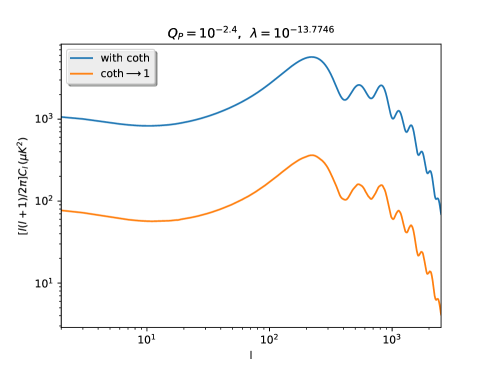
Figure 7: Angular power spectra for warm inflation for the same values of $Q_{P}$ and $\lambda$ are plotted using CAMB, with the coth term retained in the primordial power spectrum for the upper blue curve and with the coth term set to 1 for the lower orange curve. One sees that the effect of the coth term is to enhance the angular power spectrum, and it is almost uniform across angular scales. The parameters $Q_{P}$ and $\lambda$ are appropriately chosen such that at the pivot scale the primordial power spectrum associated with the blue curve is normalised.

Because the coth term shows only some variation with $k$, it effectively readjusts the normalisation of the prefactor in the power spectrum, i.e., it lowers $H$. For $N_{P}=50$ and fixed $A_{s}$, and $Q_{P}=10^{-2.4}$ for warm inflation, we have calculated the parameters of warm inflation with the coth term retained, with the coth term set to 1, and for cold inflation. The $\lambda,\phi_{P}$ and $H_{P}$ are $(1.68\times 10^{-14},3.01M_{Pl},4.09\times 10^{13}{\rm GeV}),(3.09\times 10^{-13},3.01M_{Pl},1.76\times 10^{14}{\rm GeV})$ and $(6.14\times 10^{-14},4.03M_{Pl},1.40\times 10^{14}{\rm GeV})$ respectively for the three cases. One finds that $H_{P}$ for the warm inflation case with the coth term retained is the lowest. Lower $H_{P}$ lowers the tensor power spectrum and hence the tensor to scalar ratio, $r$, thereby making the quartic potential warm inflation scenario with the coth term retained more compatible with Planck data. Quartic warm inflation with $n(k)=0$, and quartic cold inflation, give too large values of $r$ and are incompatible with the data, as also shown in Ref. [27].

5.2.1 Recovering cold inflation

For $Q_{P}<10^{-10}$ the value of $\lambda$ does not change with $Q_{P}$ for fixed $N_{P}$ and $A_{s}$ indicating that perhaps one has achieved the cold inflation limit. Indeed we find that the value of $\lambda$ and $n_{s}$ for $Q_{P}=10^{-10}$ are $5.96\times 10^{-14}$ and 0.94 and the corresponding numbers for cold inflation are very similar at $6.14\times 10^{-14}$ and 0.94. Note that for such small $Q_{P}$, $T/H$ is small and the coth term reduces to 1 giving a power spectrum corresponding to $n_{k}\approx 0$, as for standard cold inflation, which was also noted in Ref. [27].

6 Comparison with the existing literature

An analysis of the power spectrum and its dependence on the warm inflation model parameters is also given in Sec. III of Ref. [26]. Their Table 3 implies that $\lambda\sim C_{\phi}^{-1}\sim Q_{P}^{-0.33}$ which differs somewhat from our result in Sec. 4.2 that $\lambda\sim C_{\phi}^{-0.57}\sim Q_{p}^{-0.1}$ for $N_{P}$ equal to 50, which is corroborated by our CosmoMC analysis in Sec. §7.

In Eq. (5.23) of Ref. [40], the scalar spectral index for $Q_{P}\ll 1$ is given by the expression

$$n_{s}=1-3\epsilon_{1}+\frac{1}{(1+2n_{P}+\Delta_{Q})}4n_{P}\ \epsilon_{1}+\frac{1}{(1+2n_{P}+\Delta_{Q})}7\epsilon_{1}\Delta_{Q}\,,$$ (6.1)

where

$$\Delta_{Q}=2\pi Q_{P}\frac{T_{P}}{H_{P}}.$$

We have plotted our expression for $n_{s}$ in Eq. (4.2) , and that in Eq. (6.1), as a function of $Q_{P}$ in Figure (8) for $Q_{P}\leq 0.1$. One sees significant differences in the plots.

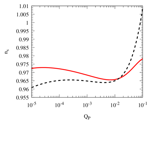
Figure 8: $n_{s}$ vs $Q_{P}$ from our expression in Eq. (4.2) (red solid line), and from that of Ref. [40] in Eq. (6.1) (black dashed line) for $N_{P}=50$ and fixed $A_{s}$.

The expression in Ref. [40] is obtained using certain approximations and hence does not include certain factors and terms. First of all, because of the coth$\left(\frac{H}{2T}\right)\sim\frac{T}{2H}$ for $H\ll 2T$ approximation , a factor $\frac{e^{H_{P}/T_{P}}}{e^{H_{P}/T_{P}}-1}\frac{H_{P}}{T_{P}}$ was missed by the authors. This factor varies from 1 to 1.4 as $Q_{P}$ goes from $10^{-1}$ to $10^{-5}$. Secondly, Eq. (6.1) is valid only in the $Q_{P}\ll 1$ approximation which is indicated by the statement just above their Eq. (5.23). If the approximation $Q_{P}\ll 1$ is not considered and $1+Q_{P}$ is retained in the derivation, an extra term $\frac{10\epsilon_{1}Q_{P}}{(1+7Q_{P})(1-\epsilon_{1})}$ is obtained as in our Eq. (4.2). This extra term is significant, $\Delta n_{s}\geq 0.005$, for $Q_{P}>10^{-1.8}$. Thirdly, in Ref. [40] the spectral index is defined as $d\ln P_{\cal R}/dN$ instead of $d\ln P_{\cal R}/d\ln(k/k_{P})$, because of which another factor of $dN/dx=-(1-\epsilon_{1})^{-1}$, as given in Eq. (3.17), is ignored . The magnitude of this overall factor varies from 1.05 to 1.02 for $Q_{P}$ between $10^{-1}$ to $10^{-5}$. In all, the combined effect of these three factors is seen in Figure (8). In the $Q_{P}\ll 1$ limit, and if we drop the factor $\frac{e^{H_{P}/T_{P}}}{e^{H_{P}/T_{P}}-1}\frac{H_{P}}{T_{P}}$, our expression for the spectral index agrees with that in Ref. [40] which implies that Eq. (6.1) is equivalent to Eq. (4.2) combined with the above approximations.

7 Constraining the parameters of the warm quartic chaotic inflation model with the full Planck 2015 data

As we saw in Section §3.1, for warm inflation driven by a single scalar field with a quartic self-interaction potential, for a given $N_{P}$ the parameters which determine the underlying microphysics can be chosen to be $Q_{P}$ and $\lambda$. We therefore obtain the joint and marginal distributions of these parameters and constrain their values.

It is well known that in cold inflation driven by a quartic potential, the self coupling $\lambda$ is quite small (${\cal O}(10^{-14}))$. From our preliminary analysis with CAMB we have found that $\lambda$ for warm inflation is similarly small. Hence we work with $-\log_{10}\lambda$ rather than $\lambda$ as one of the variables in performing our analysis. In the weak dissipative regime $Q_{P}\ll 1$ and we use $-\log_{10}Q_{P}$ as another variable. We can now attempt to constrain $-\log_{10}\lambda$ and $-\log_{10}Q_{P}$ for the two choices of $N_{P}$ i.e. $N_{P}=50$ and $N_{P}=60$.

For $N_{P}=50$ and 60, we use $10^{-14}$ to $10^{-13}$ and $10^{-14.5}$ to $10^{-13.5}$ respectively as the range of values for $\lambda$. The angular power spectrum is sensitive to $\lambda$ and we have to choose a narrow range. As discussed in Section §4.3 for the values of $Q_{P}$ smaller than $10^{-5}$, one has $T<H$ and so this regime can not be thought of as a realisation of warm inflation. Keeping this in mind, we would like to consider $Q_{P}$ between $10^{-5}$ and $10^{-1}$. However for numerical reasons we consider $-\log_{10}Q_{p}$ between 5.4 and 1 for both $N_{P}=50$ and 60.

In the Planck 2015 likelihood analysis [41] the CMB angular power spectra at low-l are computed following a Gibbs sampling approach called COMMANDER. At high-l, the TT, TE and EE power spectra are computed by using the code Plik which computes “Pseudo-Cls” by cross-correlating the data from different frequency maps. Plik has a large number nuisance parameters, representing the foreground, calibration, etc., for computing likelihood. Although the parameters of Plik also can be estimated from the Planck 2015 data in a CosmoMC analysis we have decided not to do that and fixed their values to be the best fit values for the standard $\Lambda$CDM baseline model as given by the Planck collaboration. We carry out our MCMC search in a six dimensional parameter space with the standard parameters $\Omega_{b}h^{2},\Omega_{c}h^{2},\theta,\tau$, and our parameters $-\log_{10}\lambda$ and $-\log_{10}Q_{p}$. $\Omega_{b}h^{2},\Omega_{c}h^{2},\theta$ and $\tau$ represent the baryon density, cold dark matter density, the ratio of the size of the sound horizon at decoupling ($r_{dec}$) and the angular diameter distance at decoupling ($D_{A}$), and the Thomson scattering optical depth due to reionization respectively. The priors for the standard parameters are found by comparing the CMB angular power spectra for a set of trial values with the observational data points using CAMB. We consider flat priors for all these parameters. We use the November 2016 version of CAMB and the July 2015 version of CosmoMC and set the flags, compute_tensor=T, CMB_lensing=T, and use_nonlinear_lensing=F. We use as the pivot scale $k_{P}=0.05\text{Mpc}^{-1}$, set the number of massless neutrino species to its value in the Standard Model i.e. $n_{\nu}=3.046$ and similarly set the value of the Helium fraction $Y_{He}=0.24$ in our analysis.

We present the mean and 68 % limits for the six parameters we consider in Table 1. The mean values of $\lambda$ for $N_{P}=50$ and 60 are $1.6\times 10^{-14}$ and $1.0\times 10^{-14}$ respectively, and of $Q_{P}$ are $3.7\times 10^{-3}$ and $4.4\times 10^{-3}$ respectively. We also show the marginalized probability distributions and the joint probability distribution of these parameters in Figure (9). We find that both the parameters of the quartic warm inflation model that we consider, $\lambda$ and $Q_{P}$, are well constrained by the Planck 2015 temperature and polarization data. The shape of the joint probability distribution of $-\log_{10}\lambda$ and $-\log_{10}Q_{P}$ in Figure (9) is best understood by comparing with the $\log_{10}\lambda$ vs $\log_{10}Q_{P}$ plot in Figure (4), and is consistent with the empirical relation $\lambda\sim Q_{p}^{-0.1}$ for $N_{P}=50$ and 60 obtained in Section §4.4.

S. No.	Parameter	Priors	$N_{P}=50$	$N_{P}=60$
1	$\Omega_{b}h^{2}$	(0.005,0.1)	$0.02220\pm 0.00013$	$0.02226\pm 0.00013$
2	$\Omega_{c}h^{2}$	(0.001,0.99)	$0.1191\pm 0.0010$	$0.1177\pm 0.0009$
3	$100\theta$	(0.50,10.0)	$1.04089\pm 0.00029$	$1.04105\pm 0.00029$
4	$-\log_{10}\lambda$	(13.0,14.0),(13.5,14.5)	$13.783\pm 0.051$	$13.998\pm 0.037$
5	$-\log_{10}Q_{P}$	(1.0,5.4)	$2.4358\pm 0.5856$	$2.3585\pm 0.4495$
6	$\tau$	(0.1,0.8)	$0.065\pm 0.011$	$0.075\pm 0.011$

Table 1: From the Planck 2015 TT, TE, EE + low P + lensing data mean and 68% limits for the four standard and two extra parameters of the quartic model of warm inflation for 50 and 60 number of e-foldings is displayed. The priors for various parameters are also included. (For $-\log_{10}\lambda$ separate priors for $N_{P}=50$ and 60 are indicated.)

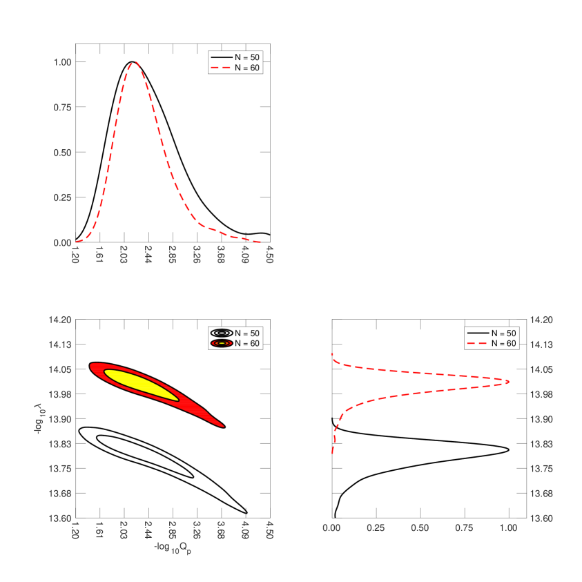
Figure 9: The joint probability distribution and the marginalized distributions for $\lambda$ and $Q_{p}$. For the marginalized distributions the black solid lines are for $N_{P}=50$ and the red dashed lines are for $N_{P}=60$. In the contour plots of the joint probability distributions the lower contours are for $N_{P}=50$ and the upper ones are for $N_{P}=60$.

A CosmoMC analysis of warm inflation for different potentials was carried out in Ref. [42]. In that analysis the CosmoMC parameters are $\Omega_{c}h^{2}$, $\Omega_{b}h^{2}$, $\theta$, $\tau$ and $Q_{P}$, for fixed $N_{P}$. The normalization of the power spectrum at the pivot scale is also taken to be fixed. In the power spectrum, the authors parametrize $Q_{k}$, $T_{k}/H_{k}$ and the prefactor in the power spectrum, $P_{0}(k)=[H_{k}^{2}/(2\pi\dot{\phi}_{k})]^{2}$, as $a_{i}k^{b_{i}+c_{i}\ln(k)}$ with $i$ referring to $Q_{k}$, $T_{k}/H_{k}$ and $P_{0}(k)$ . For each value of $Q_{P}$, and fixed $P_{\cal R}(k_{P})$ and $N_{P}$, their background equations [Eqs. (2.1-2.3, 2.9-2.15)] are used to (uniquely) determine $a_{i},b_{i}$ and $c_{i}$. With the values of these coefficients $P_{\mathcal{R}}(k)$ is known, which is used by CosmoMC. CosmoMC then provides a likelihood curve for $Q_{P}$, as shown in their Fig. 8. The algorithm BOBYQA (Bound Optimization BY Quadratic Approximation) is used to find the best fit value. Furthermore they obtain $n_{s},n_{s}^{\prime}$ and $n_{s}^{{}^{\prime\prime}}$ at $k_{P}$ using their Eqs. (2.23-2.25). Planck 2015 results suggest a lower value of the tensor to scalar $r$, and a positive value of the running of the running parameter $n_{s}^{{}^{\prime\prime}}$ (albeit of small statistical significance) and these cannot be explained in the standard cold inflation scenario driven by a quartic potential. In Ref. [42] it has been shown that different warm inflation models can explain these features, though not quartic warm inflation.

In the present work, instead of restricting our attention to finding only the best fit value of $Q_{P}$ (and then the other derived parameters), we vary both $Q_{P}$ and $\lambda$. This allows us to get the joint probability distribution for the two parameters which describe the underlying microphysics of the quartic chaotic warm inflation model. Furthermore, we do the full CosmoMC and not just BOBYQA. This allows us to get the mean values and standard deviations. In algorithms such as those followed in CosmoMC the range of preferred values, represented by the mean and standard deviation, carry more information than the best fit value.

8 Discussion and Conclusions

The standard cold inflation is based on the simple picture in which the inflaton does not experience any dissipative dynamics as it slowly rolls down during the inflationary phase. On the other hand, warm inflation provides an example of an alternative picture, in which the dissipative dynamics plays a major role even during slow roll. The next generation CMB experiments will provide unprecedentedly stringent constraints on the various parameters characterizing the primordial power spectrum of large field inflationary scenarios [43, 44]. Given this, it is important to understand how these constraints are to be interpreted, i.e. what will these constraints teach us about the epoch of cosmic inflation. Keeping this future prospect in mind, one must first best understand how the current available data constrains the possibility of warm inflation.

In this work, we studied warm inflation driven by a scalar field with a quartic potential in the weak dissipative regime i.e. in the regime in which the inflaton decay rate is small as compared to the Hubble parameter when the modes of cosmological interest cross the horizon during inflation. We focused on constraining all aspects of this specific scenario using the most recent CMB observational data. In particular we found the joint probability distribution of $\lambda$, the self coupling of the inflaton, and $Q_{P}$, the ratio of the inflaton decay width and (three times) the Hubble parameter during inflation, evaluated at the pivot scale (0.05 ${\rm Mpc}^{-1}$). We also found the mean and standard deviation values of these parameterss. $Q_{P}$ is also related to $C_{\phi}$, a parameter related to the inflaton coupling to other fields and the number of other fields in the warm inflation model.

From the marginalised distributions of the parameters of the model we find that the preferred range of values of $\lambda$ is $1.5\times 10^{-14}$ to $1.9\times 10^{-14}$ with a mean value of $1.6\times 10^{-14}$ for the number of e-foldings of inflation after the pivot scale crosses the horizon during inflation, $N_{P}$, equal to 50, and the preferred range of values for $N_{P}$ equal to 60 is $9.2\times 10^{-15}$ to $1.1\times 10^{-14}$ with a mean value of $1.0\times 10^{-14}$. The preferred range of values of $Q_{P}$ is $9.5\times 10^{-4}$ to $1.4\times 10^{-2}$ with a mean value of $3.7\times 10^{-3}$ for $N_{P}$ equal to 50, and the preferred range of values for $N_{P}$ equal to 60 is $1.6\times 10^{-3}$ to $1.2\times 10^{-2}$ with a mean value of $4.4\times 10^{-3}$. The values of $C_{\phi}$ corresponding to the mean values of $Q_{P}$ are $8.7\times 10^{6}\,(1.2\times 10^{7})$ for $N_{P}$ equal to 50 (60), from the analysis in Sec. §4.2.

From the joint probability distribution obtained using CosmoMC, as well us from the analysis of the power spectrum, normalised at the pivot scale, in Secs. 4.2 and 4.4, we obtain $\lambda\sim Q_{P}^{-0.1}$ for both $N_{P}=50$ and 60, a potentially useful result for warm inflation model building.

Acknowledgements: It is a pleasure to acknowledge discussions with Arjun Berera, Mar Bastero-Gil and Rudnei Ramos about details of their work on the warm inflationary scenario. J.P. would like to thank the Navajbai Ratan Tata Trust (NRTT) for financial support. Numerical work for the present study was done on the IUCAA HPC facility.

Note: While this manuscript was being prepared, Ref. [45] appeared on the arXiv. They too consider a CosmoMC analysis of warm inflation. They consider an inflaton dissipation rate proportional to the temperature $T$, while above we consider $\Upsilon\sim T^{3}$.

References

- [1] A. A. Starobinsky, “A New Type of Isotropic Cosmological Models Without Singularity,” Phys. Lett. 91B, 99 (1980).
- [2] D. Kazanas, “Dynamics of the Universe and Spontaneous Symmetry Breaking,” Astrophys. J. 241, L59 (1980).
- [3] A. H. Guth, “The Inflationary Universe: A Possible Solution to the Horizon and Flatness Problems,” Phys. Rev. D 23, 347 (1981).
- [4] A. D. Linde, “A New Inflationary Universe Scenario: A Possible Solution of the Horizon, Flatness, Homogeneity, Isotropy and Primordial Monopole Problems,” Phys. Lett. 108B, 389 (1982).
- [5] A. Albrecht and P. J. Steinhardt, “Cosmology for Grand Unified Theories with Radiatively Induced Symmetry Breaking,” Phys. Rev. Lett. 48, 1220 (1982).
- [6] A. A. Starobinsky, “Spectrum of relict gravitational radiation and the early state of the universe,” JETP Lett. 30, 682 (1979) [Pisma Zh. Eksp. Teor. Fiz. 30, 719 (1979)].
- [7] S. W. Hawking, “The Development of Irregularities in a Single Bubble Inflationary Universe,” Phys. Lett. 115B, 295 (1982).
- [8] A. A. Starobinsky, “Dynamics of Phase Transition in the New Inflationary Universe Scenario and Generation of Perturbations,” Phys. Lett. 117B, 175 (1982).
- [9] A. H. Guth and S. Y. Pi, “Fluctuations in the New Inflationary Universe,” Phys. Rev. Lett. 49, 1110 (1982).
- [10] A. Berera and L. Z. Fang, “Thermally induced density perturbations in the inflation era,” Phys. Rev. Lett. 74, 1912 (1995) [astro-ph/9501024].
- [11] A. Berera, “Warm inflation,” Phys. Rev. Lett. 75, 3218 (1995) [astro-ph/9509049].
- [12] A. Berera, “Warm inflation at arbitrary adiabaticity: A Model, an existence proof for inflationary dynamics in quantum field theory,” Nucl. Phys. B 585, 666 (2000) [hep-ph/9904409].
- [13] D. Lopez Nacir, R. A. Porto, L. Senatore and M. Zaldarriaga, “Dissipative effects in the Effective Field Theory of Inflation,” JHEP 1201, 075 (2012) [arXiv:1109.4192 [hep-th]].
- [14] A. Berera, M. Gleiser and R. O. Ramos, “A First principles warm inflation model that solves the cosmological horizon / flatness problems,” Phys. Rev. Lett. 83, 264 (1999) [hep-ph/9809583].
- [15] M. Bastero-Gil, A. Berera and N. Kronberg, “Exploring the Parameter Space of Warm-Inflation Models,” JCAP 1512, 046 (2015) [arXiv:1509.07604 [hep-ph]].
- [16] H. Mishra, S. Mohanty and A. Nautiyal, “Warm natural inflation,” Phys. Lett. B 710, 245 (2012) [arXiv:1106.3039 [hep-ph]].
- [17] M. Bastero-Gil, A. Berera, R. O. Ramos and J. G. Rosa, “Warm Little Inflaton,” Phys. Rev. Lett. 117, 151301 (2016) [arXiv:1604.08838 [hep-ph]].
- [18] A. Lewis and S. Bridle, “Cosmological parameters from CMB and other data: A Monte Carlo approach,” Phys. Rev. D 66, 103511 (2002) [astro-ph/0205436].
- [19] I. G. Moss and C. Xiong, “Dissipation coefficients for supersymmetric inflatonary models,” hep-ph/0603266.
- [20] M. Bastero-Gil, A. Berera and R. O. Ramos, “Dissipation coefficients from scalar and fermion quantum field interactions,” JCAP 1109, 033 (2011) [arXiv:1008.1929 [hep-ph]].
- [21] M. Bastero-Gil, A. Berera, R. O. Ramos and J. G. Rosa, “General dissipation coefficient in low-temperature warm inflation,” JCAP 1301, 016 (2013) [arXiv:1207.0445 [hep-ph]].
- [22] R. O. Ramos and L. A. da Silva, “Power spectrum for inflation models with quantum and thermal noises,” JCAP 1303, 032 (2013) [arXiv:1302.3544 [astro-ph.CO]].
- [23] E. W. Kolb and M. S. Turner, “The Early Universe”, Front. Phys. 69, 1 (1990).
- [24] A. Berera, I. G. Moss and R. O. Ramos, “Warm Inflation and its Microphysical Basis,” Rept. Prog. Phys. 72, 026901 (2009) [arXiv:0808.1855 [hep-ph]].
- [25] C. Graham and I. G. Moss, “Density fluctuations from warm inflation,” JCAP 0907, 013 (2009) [arXiv:0905.3500 [astro-ph.CO]].
- [26] M. Bastero-Gil and A. Berera, “Warm inflation model building,” Int. J. Mod. Phys. A 24, 2207 (2009) [arXiv:0902.0521 [hep-ph]].
- [27] S. Bartrum, M. Bastero-Gil, A. Berera, R. Cerezo, R. O. Ramos and J. G. Rosa, “The importance of being warm (during inflation),” Phys. Lett. B 732, 116 (2014) [arXiv:1307.5868 [hep-ph]].
- [28] A. Berera, M. Gleiser and R. O. Ramos, “Strong dissipative behavior in quantum field theory,” Phys. Rev. D 58, 123508 (1998) [hep-ph/9803394].
- [29] J. Yokoyama and A. D. Linde, “Is warm inflation possible?,” Phys. Rev. D 60, 083509 (1999) [hep-ph/9809409].
- [30] D. J. Schwarz, C. A. Terrero-Escalante and A. A. Garcia, “Higher order corrections to primordial spectra from cosmological inflation,” Phys. Lett. B 517, 243 (2001) [astro-ph/0106020].
- [31] I. G. Moss and C. Xiong, “On the consistency of warm inflation,” JCAP 0811, 023 (2008) [arXiv:0808.0261 [astro-ph]].
- [32] L. M. Hall, I. G. Moss and A. Berera, “Scalar perturbation spectra from warm inflation,” Phys. Rev. D 69, 083525 (2004) [astro-ph/0305015].
- [33] I. G. Moss, “Primordial Inflation With Spontaneous Symmetry Breaking,” Phys. Lett. 154B, 120 (1985).
- [34] M. Bastero-Gil, A. Berera and R. O. Ramos, “Shear viscous effects on the primordial power spectrum from warm inflation,” JCAP 1107, 030 (2011) [arXiv:1106.0701 [astro-ph.CO]].
- [35] S. Bartrum, A. Berera and J. G. Rosa, “Gravitino cosmology in supersymmetric warm inflation,” Phys. Rev. D 86, 123525 (2012) [arXiv:1208.4276 [hep-ph]].
- [36] P. A. R. Ade et al. [Planck Collaboration], “Planck 2015 results. XIII. Cosmological parameters,” Astron. Astrophys. 594, A13 (2016) [arXiv:1502.01589 [astro-ph.CO]] (Table 4).
- [37] http://camb.info/
- [38] P. A. R. Ade et al. [Planck Collaboration], “Planck 2013 results. XV. CMB power spectra and likelihood,” Astron. Astrophys. 571, A15 (2014) [arXiv:1303.5075 [astro-ph.CO]].
- [39] K. Bhattacharya, S. Mohanty and R. Rangarajan, “Temperature of the inflaton and duration of inflation from WMAP data,” Phys. Rev. Lett. 96, 121302 (2006) [hep-ph/0508070].
- [40] M. Bastero-Gil, A. Berera, I. G. Moss and R. O. Ramos, “Cosmological fluctuations of a random field and radiation fluid,” JCAP 1405, 004 (2014) [arXiv:1401.1149 [astro-ph.CO]].
- [41] N. Aghanim et al. [Planck Collaboration], “Planck 2015 results. XI. CMB power spectra, likelihoods, and robustness of parameters,” Astron. Astrophys. 594, A11 (2016) [arXiv:1507.02704 [astro-ph.CO]].
- [42] M. Benetti and R. O. Ramos, “Warm inflation dissipative effects: predictions and constraints from the Planck data,” Phys. Rev. D 95, 023517 (2017) [arXiv:1610.08758 [astro-ph.CO]].
- [43] K. N. Abazajian et al. [CMB-S4 Collaboration], “CMB-S4 Science Book, First Edition,” arXiv:1610.02743 [astro-ph.CO].
- [44] J. B. Muñoz, E. D. Kovetz, A. Raccanelli, M. Kamionkowski and J. Silk, “Towards a measurement of the spectral runnings,” JCAP 1705, 032 (2017) [arXiv:1611.05883 [astro-ph.CO]].
- [45] M. Bastero-Gil, S. Bhattacharya, K. Dutta and M. R. Gangopadhyay, “Constraining Warm Inflation with CMB data,” arXiv:1710.10008 [astro-ph.CO].