Prediction of Satisfied User Ratio for Compressed Video

Abstract

A large-scale video quality dataset called the VideoSet has been constructed recently to measure human subjective experience of H.264 coded video in terms of the just-noticeable-difference (JND). It measures the first three JND points of 5-second video of resolution 1080p, 720p, 540p and 360p. Based on the VideoSet, we propose a method to predict the satisfied-user-ratio (SUR) curves using a machine learning framework. First, we partition a video clip into local spatial-temporal segments and evaluate the quality of each segment using the VMAF quality index. Then, we aggregate these local VMAF measures to derive a global one. Finally, the masking effect is incorporated and the support vector regression (SVR) is used to predict the SUR curves, from which the JND points can be derived. Experimental results are given to demonstrate the performance of the proposed SUR prediction method.

Index Terms—  Video Quality Assessment, Satisfied User Ratio, Just Noticeable Difference

1 Introduction

A large amount of bandwidth of fixed and mobile networks is consumed by real-time video streaming. It is desired to lower the bandwidth requirement by taking human visual perception into account. Although the peak signal-to-noise ratio (PSNR) has been used as an objective measure in video coding standards for years, it is generally agreed that it is a poor visual quality metric that does not correlate with human visual experience well [1].

There has been a large amount of efforts in developing new visual quality indices to address this problem, including SSIM [2], FSIM [3], DLM [4], etc. Humans are asked to evaluate the quality of visual contents by a set of discrete or continuous values called opinion score; typical opinion scores in the range 1-5, with 5 being the best and 1 the worst quality. These indices offer, by definition, users’ subjective test results and thus correlate better than PSNR with their mean (called mean opinion score, or MOS). However, there is one shortcoming with these indices. That is, the difference of selected contents for ranking is sufficiently large for a great majority of subjects. Since the difference is higher than the just-noticeable-difference (JND) threshold for most people, disparities between visual content pairs are easier to tell.

Humans cannot perceive small pixel variation in coded image/video until the difference reaches a certain level. There is a recent trend to measure the JND threshold directly for each individual subject. The idea was first proposed in [5]. An assessor is asked to compare a pair of coded image/video contents and determine whether they are the same or not in the subjective test, and a bisection search is adopted to reduce the number of comparisons. Two small-scale JND-based image/video quality datasets were built by the Media Communications Lab at the University of Southern California. They are the MCL-JCI dataset [6] and the MCL-JCV dataset [7]. They target at the JND measurement of JPEG coded images and H.264/AVC coded video, respectively.

The number of JPEG coded images reported in [6] is 50 while the number of subjects is 30. The distribution of multiple JND points were modeled by a Gaussian Mixture Model (GMM) in [8], where the number of mixtures was determined by the Bayesian Information Criterion (BIC). The MCL-JCV dataset in [7] consists of 30 video clips of wide content variety and each of them were evaluated by 50 subjects. Differences between consecutive JND points were analyzed with outlier removal. It was also shown in [7] that the distribution of the first JND samples of multiple subjects can be well approximated by the normal distribution. The JND measure was further applied to the HEVC coded clips and, more importantly, a JND prediction method was proposed in [9]. The masking effect was considered, related features were derived from source video, and a spatial-temporal sensitive map (STSM) was defined to capture the unique characteristics of the source content. The JND prediction problem was treated as a regression problem.

More recently, a large-scale JND-based video quality dataset, called the VideoSet, was built and reported in [10]. The VideoSet consists of 220 5-second sequences, each at four resolutions (i.e., $1920\times 1080$, $1280\times 720$, $960\times 540$ and $640\times 360$). Each of these 880 video clips was encoded by the x264 encoder implementation [11] of the H.264/AVC standard with $QP=1,\cdots,51$ and the first three JND points were evaluated by 30+ subjects. The VideoSet dataset is available to the public in the IEEE DataPort [10]. It includes all source/coded video clips and measured JND data.

In this work, we focus on the prediction of the satisfied user ratio (SUR) curves for the VideoSet and derive the JND points from the predicted curves. This is different from the approach in [9], which attempted to predict the JND point directly. Here, we adopt a machine learning framework for the SUR curve prediction. First, we partition a video clip into local spatial-temporal segments and evaluate the quality of each segment using the VMAF [12] quality index. Then, we aggregate these local VMAF measures to derive a global one. Finally, the masking effect is incorporated and the support vector regression (SVR) is used to predict the SUR curves, from which the JND points can be derived. Experimental results are given to demonstrate the performance of the proposed SUR prediction method.

The rest of this paper is organized as follows. The SUR curve prediction problem is defined in Sec. 2. The SUR prediction method is detailed in Sec. 3. Experimental results are provided in Sec. 4. Finally, concluding remarks and future research direction are given in Sec. 5.

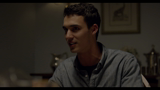
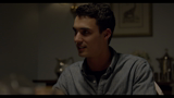
(a)

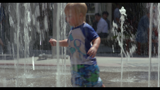
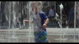
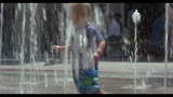
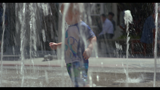
(b)

Fig. 1: Representative frames from source sequences (a) #37 and (b) #89.

2 JND and SUR for Coded Video

Given a set of clips $d_{i}$, $i=0,1,2,\cdots,51$, coded from the same source video $r$, where $i$ is the quantization parameter (QP) index used in the H.264/AVC. Typically, clip $d_{i}$ has a higher PSNR value than clip $d_{j}$, if $i<j$, and $d_{0}$ is the losslessly coded copy of $r$. The first JND location is the transitional index $i$ that lies on the boundary of perceptually lossless and lossy visual experience for a subject. The first JND is a random variable rather than a fixed quantity since it varies with several factors, including the visual content under evaluation, the test subject and the test environment. Based on the study in [10], the JND position can be approximated by a Gaussian distribution in form of

$$X\sim\mathcal{N}(\bar{x},s^{2}),$$ (1)

where $\bar{x}$ and $s$ are the sample mean and sample standard deviation, respectively.

We say that a viewer is satisfied if the compressed video appears to be perceptually the same as the reference. Mathematically, the satisfied user ratio (SUR) of vide clip $d_{i}$ can be expressed as

$$S_{i}=1-\frac{1}{M}\sum_{m=1}^{M}\mathds{1}_{m}(d_{i}),$$ (2)

where $M$ is the total number of subjects and $\mathds{1}_{m}(d_{i})=1$ or $0$ if the $m$th subject can or cannot see the difference between compressed clip $d_{i}$ and its reference, respectively. The summation term in right-hand-side of Eq. (2) is the empirical cumulative distribution function (CDF) of random variable $X$ as given in Eq. (1). Then, by plugging Eq. (1) into Eq. (2), we can obtain a compact formula for the SUR curve as

$$S_{i}=Q(d_{i}|\bar{x},s^{2}),$$ (3)

where $Q(\cdot)$ is the Q-function of the normal distribution.

3 Proposed SUR prediction System

The SUR curve is primarily determined by two factors: 1) quality degradation due to compression and 2) the masking effect. To shed light on the impact of the masking effect, we use sequences #37 (DinnerTable) and #89 (TodderFountain) as examples. Their representative frames are shown in Figs. 1 (a) and (b) and their JND data distributions are given in Figs. 2 (a) and (b), respectively. Sequence #37 is a scene captured around a dining table. It focuses on a male speaker with still dark background. His face is the visual salient region that attracts people’s attention. The masking effect is weak and, as a result, the JND point arrives earlier (i.e. a smaller $i$ value in $d_{i}$). On the other hand, sequence #89 is a scene about a toddler playing in a fountain. The masking effect is strong due to water drops in background and fast object movement. As a result, compression artifacts are difficult to perceive and the JND point arrives later.

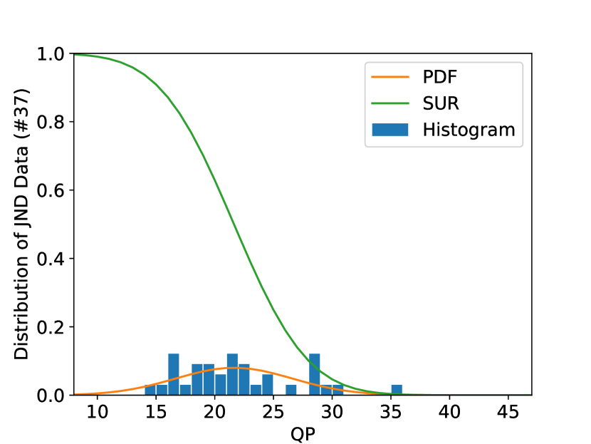
(a)

(b)

Fig. 2: SUR modeling from JND samples. The JND histogram (in blue), the smoothed PDF curve (in orange) and the SUR curve (in green) for sequences (a) #37 and (b) #89.

The block diagram of the proposed SUR prediction system is given in Fig. 3. When a subject evaluates a pair of video clips, different spatial-temporal segments of the two video clips are successively assessed. The segment dimensions are spatially and temporally bounded. The spatial dimension is determined by the area where the sequence is projected on the fovea. The temporal dimension is limited by the fixation duration or the smooth pursuit duration, where the noticeable difference is more likely to happen than the process of saccades [13, 14]. Thus, the proposed SUR prediction system first evaluates the quality of local Spatial-Temporal Segments. Then, similarity indices in these local segments are aggregated to give a compact global index. Then, significant segments are selected based on the slope of quality scores between neighboring coded clips. After that, we incorporate the masking effect that reflects the unique characteristics of each video clip. Finally, we use the support vector regression (SVR) to minimize the $L_{2}$ distance of the SUR curves, and derive the JND point accordingly. Several major modules of the system will be detailed below.

Fig. 3: The block diagram of the proposed SUR prediction system.

Step 1. Spatial-Temporal Segment Creation

The purpose of this module is to divide a video clip into multiple spatial-temporal segments and evaluate their quality at the eye fixation level. The dimension of a spatial-temporal segment is $W\times H\times T$. In case of eye pursuit, the spatial dimension should be large enough while the temporal dimension should be short enough to ensure that the moving object is still covered in one segment. In case of eye fixation, the spatial dimension should not be too large and the temporal dimension should not be too long to represent quality well at the fixation level. Based on the study in [15, 14], we set $W=320$, $H=180$ and $T=0.5s$ here. The neighboring segments overlap 50% in the spatial dimension. For example, the original dimension of 720p video is $1280\times 720\times 5s$, and there are $7\times 7\times 10=490$ segments created from each clip.

Step 2. Local Quality Assessment

We choose the Video Multimethod Assessment Fusion (VMAF) [12] as the primary quality index to assess quality degradation of compressed segments. VMAF is an open-source full-reference perceptual video quality index that aims to capture the perceptual quality of compressed video. It first estimates the quality score of a video clip with multiple high-performance image quality indices on a frame-by-frame basis. Then, these image quality scores are fused together using the support vector machine (SVM) at each frame. Results on various video quality databases show that VMAF outperforms other video quality indices such as PSNR, SSIM [2], Multiscale Fast-SSIM [16], and PSNR-HVS [17] in terms of the Spearman Rank Correlation Coefficient (SRCC), Pearson Correlation Coefficient (PCC), and the root-mean-square error (RMSE) criteria. VMAF achieves comparable or outperforms the state-of-the-art video index, the VQM-VFD index [15], on several publicly available databases. For more details about VMAF, we refer interested readers to [12].

Step 3. Significant Segments Selection

VMAF is typically applied to all spatial-temporal segments. However, not all segments contribute equally to the final quality of the entire clip. To select significant segments that are more relevant to our objective, we examine the local quality degradation slope, which is defined as

$$\delta V(S_{wht}^{d_{i}})=\frac{V(S_{wht}^{d_{i-k}})-V(S_{wht}^{d_{i}})}{k},$$ (4)

where $V(S_{wht}^{d_{i}})$ is the VMAF score of segment $S_{wht}^{d_{i}}$ that is cropped from compressed clip $d_{i}$ with spatial indices $(w,h)$ and temporal index $t$, respectively. The slope in Eq. (4) evaluates how much the VMAF score of the current segment $S_{wht}^{d_{i}}$ differs from that in its neighboring compressed clip $S_{wht}^{d_{i-k}}$, where $k=2$ is the QP difference between them. If the slope is small, the local quality does not change too much and the probability of the associated coding index $i$ to be a JND point is lower. We order all spatial-temporal segments based on their slopes and select $p$ percents of them with larger slope values. We set $p=80\%$ in our experiment. The goal is to filter out less important segments before we extract a representative feature vector.

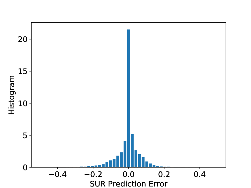
(a)

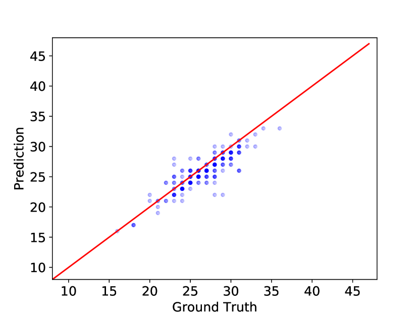
(b)

Fig. 4: JND prediction result: (a) the histogram of $\Delta$ SUR and (b) the predicted VS. the ground truth JND location.

Step 4. Quality Degradation Features

A cumulative quality degradation curve is computed for every coded clip based on the change of VMAF scores in significant segments. Its computation consists of two steps. First, we compute the difference of VMAF scores between a significant segment from compressed clip $d_{i}$ and its reference $r$ as

$$\Delta V(S_{wht}^{d_{i}})=V(S_{wht}^{r})-V(S_{wht}^{d_{i}}).$$ (5)

The values $\Delta V(S_{wht}^{d_{i}})$ collected from all significant segments can be viewed as samples of a random variable denoted by $\Delta V(S^{d_{i}})$. Then, based on the distribution of $\Delta V(S^{d_{i}})$, we can compute the cumulative quality degradation curve as

$$F^{d_{i}}(n)=Prob[\Delta V(S^{d_{i}})\leq 2n],\mbox{ for }n=1,\cdots,20,$$ (6)

which captures the cumulative histogram of VMAF score differences for coded video $d_{i}$. As shown in Eq. (6), the cumulative quality degradation curve is represented in form of a 20-D feature vector.

Step 5. Masking Features

As mentioned earlier, quality degradation in a spatial-temporal segment is more difficult to observe if there exists a masking effect in the segment. Here, we use the spatial randomness and temporal randomness proposed in [18, 19] to measure the masking effect. The process is sketched below. First, high frequency components of distortions are first removed by applying a low-pass filter, which is inspired by the Contrast Sensitivity Function (CSF), in the pre-processing step. Then, we use the spatial randomness (SR) model [18] and the temporal randomness (TR) [19] to compute the spatial and temporal regularity in a spatial-temporal segment that is generated in Step 1. The spatial randomness is small in smooth or highly structured regions. Similarly, the temporal randomness is small if there is little motion between adjacent frames. When the SR and TR values are higher, the spatial and temporal masking effects are stronger. The masking features, $M_{s}$, are extracted from the reference clip only. The histograms of the SR and the TR are concatenated to yield the final masking feature vector:

$$M^{d_{0}}=[Hist_{10}(SR),Hist_{10}(TR)].$$ (7)

Step 6. Prediction of SUR Curves and JND Points

The final feature vector is the concatenation of two feature vectors. The first one is the quality degradation feature vector of dimension 20 as given in Eq. (6). The second one is the masking feature vector of dimension 20 as given in Eq. (7). Thus, the dimension of the final concatenated feature vector is $40$. The SUR prediction problem is treated as a regression problem, and solved by the Support Vector Regressor (SVR) [20]. Specifically, we adopt the $\epsilon$-SVR with the radial basis function kernel.

4 Experimental Results

In this section, we present the prediction results of the proposed SUR prediction framework. The VideoSet consists of 220 videos in 4 resolutions and three JND points per resolution per video clip. Here, we focus on the SUR prediction of the first JND and conduct this task for each video resolution independently. For each resolution, we trained and tested 220 video clips using the 5-fold validation. That is, we choose 80% (i.e. 176 video clips) as the training set and the remaining 20% (i.e., 44 video clips) as the testing set. We rotated the 20% testing set five times so that each video clip was tested once. Since the JND location is chosen to be the QP value when the SUR value is equal to 75% in the VideoSet, we adopt the same rule here so that the JND position can be easily computed from the predicted SUR curve.

The averaged prediction errors of the SUR curve and the JND position for video clips in four resolutions were summarized in Table 1. We see that prediction errors increase as the resolution becomes lower. This is probably due to the use of fixed $W$ and $H$ values in generating spatial-temporal segments as described in Sec. 3. We will finetune these parameters to obtain better prediction results in the future.

To see the prediction performance of each individual clip, we use 720p video as an example. The histogram of the SUR prediction error is given in Fig. 4 (a), where the mean absolute error (MAE) is 0.038 for all test sequences. The predicted JND location versus the ground-truth JND location is plotted in Fig. 4 (b), where each dot denotes one video clip. As shown in the figure, most dots are distributed along the 45-degree line, which indicates that the predicted JND is very close to the ground truth JND for most sequences.

Table 1: Summary of averaged prediction errors for video clips in four resolutions.

	1080p	720p	540p	360p
$\Delta$SUR	0.039	0.038	0.037	0.042
$\Delta$QP	1.218	1.273	1.345	1.605

5 Conclusion and Future Work

A Satisfied User Ratio (SUR) prediction framework for H.264/AVC coded video was proposed in this work. It took both the local quality degradation as well as the masking effect into consideration and extract a compact feature vector and fed it into the support vector regressor to obtain the predicted SUR curve. The first JND point can be derived accordingly. The system achieves good performance in all resolutions. We will adopt the same framework to predict locations of the second and the third JND points in the near future.

References

- [1] W. Lin and C.-C. Jay Kuo, “Perceptual visual quality metrics: A survey,” Journal of Visual Communication and Image Representation, vol. 22, no. 4, pp. 297–312, 2011.
- [2] Zhou Wang, A.C. Bovik, H.R. Sheikh, and E.P. Simoncelli, “Image quality assessment: from error visibility to structural similarity,” Image Processing, IEEE Transactions on, vol. 13, no. 4, pp. 600–612, April 2004.
- [3] Lin Zhang, D. Zhang, Xuanqin Mou, and D. Zhang, “FSIM: A feature similarity index for image quality assessment,” Image Processing, IEEE Transactions on, vol. 20, no. 8, pp. 2378–2386, Aug 2011.
- [4] Songnan Li, Fan Zhang, Lin Ma, and King Ngi Ngan, “Image quality assessment by separately evaluating detail losses and additive impairments,” IEEE Transactions on Multimedia, vol. 13, no. 5, pp. 935–949, 2011.
- [5] Joe Yuchieh Lin, Lina Jin, Sudeng Hu, Ioannis Katsavounidis, Zhi Li, Anne Aaron, and C-C Jay Kuo, “Experimental design and analysis of JND test on coded image/video,” in SPIE Optical Engineering+ Applications. International Society for Optics and Photonics, 2015, pp. 95990Z–95990Z.
- [6] Lina Jin, Joe Yuchieh Lin, Sudeng Hu, Haiqiang Wang, Ping Wang, Ioannis Katasvounidis, Anne Aaron, and C.-C. Jay Kuo, “Statistical study on perceived JPEG image quality via MCL-JCI dataset construction and analysis,” in IS&T/SPIE Electronic Imaging. International Society for Optics and Photonics, 2016.
- [7] H. Wang, W. Gan, S. Hu, J. Y. Lin, L. Jin, L. Song, P. Wang, I. Katsavounidis, A. Aaron, and C.-C. J. Kuo, “MCL-JCV: A JND-based H.264/AVC video quality assessment dataset,” in 2016 IEEE International Conference on Image Processing (ICIP), Sept 2016, pp. 1509–1513.
- [8] Sudeng Hu, Haiqiang Wang, and C-C Jay Kuo, “A GMM-based stair quality model for human perceived JPEG images,” arXiv preprint arXiv:1511.03398, 2015.
- [9] Qin Huang, Haiqiang Wang, Sung Chang Lim, Hui Yong Kim, Se Yoon Jeong, and C-C Jay Kuo, “Measure and prediction of hevc perceptually lossy/lossless boundary qp values,” in Data Compression Conference (DCC), 2017. IEEE, 2017, pp. 42–51.
- [10] Haiqiang Wang, Ioannis Katsavounidis, Jiantong Zhou, Jeonghoon Park, Shawmin Lei, Xin Zhou, Man-On Pun, Xin Jin, Ronggang Wang, Xu Wang, et al., “Videoset: A large-scale compressed video quality dataset based on jnd measurement,” Journal of Visual Communication and Image Representation, vol. 46, pp. 292–302, 2017.
- [11] Laurent Aimar, Loren Merritt, Eric Petit, Min Chen, Justin Clay, Mns Rullgrd, Christian Heine, and Alex Izvorski, “X264-a free H264/AVC encoder,” http://www.videolan.org/developers/x264.html, 2005, Accessed: 04/01/07.
- [12] Zhi Li, Anne Aaron, Ioannis Katsavounidis, Anush Moorthy, and Megha Manohara, “Toward a practical perceptual video quality metric,” The Netflix Tech Blog, vol. 6, 2016.
- [13] James E Hoffman, “Visual attention and eye movements,” Attention, vol. 31, pp. 119–153, 1998.
- [14] Alexandre Ninassi, Olivier Le Meur, Patrick Le Callet, and Dominique Barba, “Considering temporal variations of spatial visual distortions in video quality assessment,” IEEE Journal of Selected Topics in Signal Processing, vol. 3, no. 2, pp. 253–265, 2009.
- [15] Stephen Wolf and MH Pinson, “Video quality model for variable frame delay (vqm vfd),” National Telecommunications and Information Administration NTIA Technical Memorandum TM-11-482, 2011.
- [16] Ming-Jun Chen and Alan C Bovik, “Fast structural similarity index algorithm,” Journal of Real-Time Image Processing, vol. 6, no. 4, pp. 281–287, 2011.
- [17] Nikolay Ponomarenko, Flavia Silvestri, Karen Egiazarian, Marco Carli, Jaakko Astola, and Vladimir Lukin, “On between-coefficient contrast masking of dct basis functions,” in Proceedings of the third international workshop on video processing and quality metrics, 2007, vol. 4.
- [18] Sudeng Hu, Lina Jin, Hanli Wang, Yun Zhang, Sam Kwong, and C.-C.J. Kuo, “Compressed image quality metric based on perceptually weighted distortion,” Image Processing, IEEE Transactions on, vol. 24, no. 12, pp. 5594–5608, Dec 2015.
- [19] S. Hu, L. Jin, H. Wang, Y. Zhang, S. Kwong, and C. C. J. Kuo, “Objective Video Quality Assessment based on Perceptually Weighted Mean Squared Error,” IEEE Transactions on Circuits and Systems for Video Technology, vol. PP, no. 99, pp. 1–1, 2016.
- [20] Alex J Smola and Bernhard Schölkopf, “A tutorial on support vector regression,” Statistics and computing, vol. 14, no. 3, pp. 199–222, 2004.