Asymptotic degree distributions
in large (homogeneous) random networks:
A little theory and a counterexample

Abstract

In random graph models, the degree distribution of an individual node should be distinguished from the (empirical) degree distribution of the graph that records the fractions of nodes with given degree. We introduce a general framework to explore when these two degree distributions coincide asymptotically in a sequence of homogeneous random networks of increasingly large size. The discussion is carried under three basic statistical assumptions on the degree sequences: (i) distributional homogeneity; (ii) existence of an asymptotic (nodal) degree distribution; and (iii) asymptotic uncorrelatedness. It follows from the discussion that under (i)-(ii) the asymptotic equality of the two degree distributions occurs if and only if (iii) holds. We use this observation to show that the asymptotic equality may fail in some homogeneous random networks. The counterexample is found in the class of random threshold graphs for which (i) and (ii) hold but where (iii) does not. An implication of this finding is that these random threshold graphs cannot be used as a substitute to the Barabási-Albert model for scale-free network modeling, as was proposed by some authors. The results can also be formulated for non-homogeneous models by making use of a random sampling procedure over the nodes.

1 Introduction

In the past three decades considerable efforts have been devoted to understanding the rich structure and functions of complex networks, be they technologically engineered, found in nature or generated through social interactions. These developments have been recorded in surveys, e.g., [1, 19, 32], research monographs, e.g., [4, 16, 20, 25, 33], and anthologies of research papers, e.g., [34].

The questions of interest often relate to a collection of entities (alternatively called nodes, agents, etc.) and to a set of relationships between them. The pairings can be physical, logical or social in nature; when pictured as links or edges between nodes, they naturally give rise to graphs and graph-like structures (customarily referred to as networks) on the set of nodes. Often the pairwise relationships are best viewed as inherently random, suggesting that random graph models be used to frame the relevant issues – Here we understand a random graph to be a graph-valued random variable (rv).

A popular research direction has been concerned with designing random graph models that exhibit key properties observed in real networks. Historically attention has been given to the simplest of network properties, namely the degree of nodes and their various distributions. The discussion invariably starts with the work of Erdős and Rényi [22]: With $n$ nodes and link probability $p$, the (binomial) Erdős-Rényi graph $\mathbb{G}(n;p)$ postulates that the $\frac{n(n-1)}{2}$ potential undirected links between these $n$ nodes are each created with probability $p$, independently of each other. The degree distribution in Erdős-Rényi graphs is announced to be Poisson-like, the justification going roughly as follows: (i) With $D_{n,k}(p)$ denoting the degree rv of node $k$ in $\mathbb{G}(n;p)$, the rvs $D_{n,1}(p),\ldots,D_{n,n}(p)$ are identically distributed, each distributed according to a binomial rv ${\rm Bin}(n-1;p)$; (ii) If the link probability scales with $n$ as $p_{n}\sim\frac{\lambda}{n}$ for some $\lambda>0$, then Poisson convergence ensures the distributional convergence

$$D_{n,1}(p_{n})\Longrightarrow_{n}D$$ (1)

with $D$ denoting a Poisson rv with parameter $\lambda$. A rich asymptotic theory has been developed for Erdős-Rényi graphs in the many node regime; see the monographs [10, 18, 20, 26].

However, in many networks the data tells a different story: If the network comprises a large number $n$ nodes and $N_{n}(d)$ is the number of nodes with degree $d$ in the network, then statistical analysis suggests a power-law behavior of the form

$$\frac{N_{n}(d)}{n}\simeq Cd^{-\alpha}$$ (2)

for some $\alpha$ in the range $[2,3]$ (with occasional exceptions) and $C>0$. See [20, Section 4.2] for an introductory discussion and references, and the paper by Clauset et al. [15] for a principled statistical framework. Statements such as (2) are usually left somewhat vague as the range of $d$ is never carefully specified; networks where (2) was observed are often called scale-free networks.

On account of this observation, Erdős-Rényi graphs were deemed inadequate for modeling scale-free networks (as well as other networks of interest). As a result, new classes of random graph models have been proposed in an attempt to capture the behavior (2) (and other properties), e.g., the configuration model [8, 9, 30, 31], generalized random graphs [12], and exponential random graphs [24, 40] to name some of the possibilities. The Barabási-Albert network model came to prominence for its ability to formally “explain” the existence of power law degree distributions in large networks via the mechanism of preferential attachment [3].

The statement (2) concerns an empirical degree distribution computed network-wide, whereas the convergence (1) addresses the behavior of the (generic) degree of a single node, its distribution being identical across nodes. A natural question is then whether these two different points of view are compatible with each other and can be reconciled, at least asymptotically, in large networks, and if so, under what conditions. The purpose of this paper is to explore this issue in some details. What follows is an outline of some of the contributions along these lines:

1. In Section 2 a general framework to investigate this discrepancy is introduced in terms of a sequence of random graphs $\{\mathbb{G}_{n},\ n=1,2,\ldots\}$ whose size goes to infinity with $n$. Two different settings of increasing generality are considered.

2. The homogeneous setting captures situations where an asymptotic nodal degree distribution exists, and is presented in Section 3. It is defined in terms of the following three assumptions:

1. A weak form of distributional homogeneity (hence the terminology homogeneous networks): In particular, for each $n=1,2,\ldots$, the degree rvs in $\mathbb{G}_{n}$ are identically distributed across nodes – Let $D_{n}$ denote the generic degree rv in $\mathbb{G}_{n}$;

2. Existence of an asymptotic (nodal) degree distribution: In analogy with (1), there exists an $\mathbb{N}$-valued rv $D$ such that

   $$D_{n}\Longrightarrow_{n}D.$$ (3)

   Let $(p(d),\ d=0,1,\ldots)$ denote the pmf of $D$; and

3. Asymptotic uncorrelatedness: The degree rvs $\{D_{n},\ n=1,2,\ldots\}$ display a weak form of asymptotic “pairwise independence.”

3. The relevant results for the homogeneous case are discussed in Section 4. Under the aforementioned assumptions, Proposition 4.2 states that if $(P_{n}(d),\ d=0,1,\ldots)$ is the empirical degree distribution in $\mathbb{G}_{n}$ (with $P_{n}(d)$ denoting the fraction of nodes with degree $d$ in $\mathbb{G}_{n}$), then

$$P_{n}(d)\mbox{~{}$\stackrel{{\scriptstyle P}}{{\longrightarrow}}$}_{n}~{}p(d),\quad d=0,1,\ldots$$ (4)

where the pmf $(p(d),\ d=0,1,\ldots)$ on $\mathbb{N}$ is as postulated in (ii) above. A strengthening of this result in terms of total variation distance is provided as Proposition 6.1.

4. A more general setting is considered in Section 5 where degree homogeneity, namely (i) above, is replaced by a random sampling procedure over pairs of nodes. Many situations are easily fitted into this more general framework. They include the non-homogeneous Barabási-Albert model (and other growth models), sequences of deterministic graphs and sequences which are locally weakly convergent [2] (or weakly convergent in the sense of Benjamini and Schramm [5]).

5. In Section 7 we introduce a broad class of models where the underlying assumptions (i)–(iii) can be checked; this provides a natural and convenient setting for applying Proposition 4.2. Erdős-Rényi graphs (under the scaling yielding (1)) are readily subsumed in this framework, as are many other homogeneous networks of interest in applications; see [35] for details. This resolves the discrepancy mentioned earlier in that the appropriate version of (4) does hold for both Erdős-Rényi graphs (by virtue of Proposition 4.2) [35] and for the Barabási-Albert model (for which (4) holds with limiting pmf satisfying $p(d)\sim d^{-3}$ ($d\rightarrow\infty)$ [11]).

6. Next we turn our attention to the proposition, too often taken for granted, that in homogeneous random graphs the convergence (3) of the generic degree distribution automatically implies the convergence (4) of the empirical degree distribution. In Section 8 we provide a counterexample drawn from the class of random threshold graph models [13, 23, 29, 39]. For this class of models under exponentially distributed fitness, although (3) is known to take place with $p(d)\sim d^{-2}$ ($d\rightarrow\infty)$ [23], we show that (4) fails to hold. This fact, contained in Proposition 8.2, constitutes an easy byproduct of Proposition 8.1. Proofs occupy Section 10 to Section 13, and rely on the asymptotics of order statistics for i.i.d. variates [21, 28]. We illustrate this failure through limited simulation results in Section 9.

7. One implication of this last finding is that random threshold graphs with exponentially distributed fitness cannot be used as an alternative scale-free model to the Barabási-Albert model (see below) as claimed by some authors [13, 39]. Indeed, only the convergence (4) has meaning in the preferential attachment model while (3) is meaningless there, with the situation being reversed for random threshold graphs. In other words, leaving aside the issue of which value of $\alpha$ is appropriate, the two models cannot be compared in terms of their degree distributions! This highlights the fact that even in homogeneous graphs, the network-wide degree distribution and the nodal degree distribution may capture vastly different information.

Some of the results discussed in this paper were announced in the conference paper [36], mostly without proofs. Different proofs to establish Proposition 8.2. were originally given in the Ph.D. thesis of the first author [35].

2 A simple framework

First some notation and conventions: The random variables (rvs) under consideration are all defined on the same probability triple $(\Omega,{\cal F},\mathbb{P})$. The construction of a probability triple sufficiently large to carry all the required rvs is standard, and omitted in the interest of brevity. All probabilistic statements are made with respect to the probability measure $\mathbb{P}$, and we denote the corresponding expectation operator by $\mathbb{E}$. The notation $\mbox{~{}$\stackrel{{\scriptstyle P}}{{\longrightarrow}}$}_{n}$ (resp. $\Longrightarrow_{n}$) is used to signify convergence in probability (resp. convergence in distribution) (under $\mathbb{P}$) with $n$ going to infinity; see the monographs [7, 14] for definitions and properties. If $E$ is a subset of $\Omega$, then ${\bf 1}\left[E\right]$ is the indicator rv of the set $E$ with the usual understanding that ${\bf 1}\left[E\right](\omega)=1$ (resp. ${\bf 1}\left[E\right](\omega)=0$) if $\omega\in E$ (resp. $\omega\notin E$). The symbol $\mathbb{N}$ (resp. $\mathbb{N}_{0}$) denotes the set of non-negative (resp. positive) integers.

The discussion is carried out in the following framework often encountered in the literature; see Section 7 for examples: Given is a sequence of random graphs $\{\mathbb{G}_{n},\ n=2,3,\ldots\}$ defined on the probability triple $(\Omega,{\cal F},\mathbb{P})$ – We interchangeably use the terms random graphs and random networks. Fix $n=2,3,\ldots$. The random graph $\mathbb{G}_{n}$ is then an ordered pair $(V_{n},\mathbb{E}_{n})$ defined on the set of nodes $V_{n}$ with random edge set $\mathbb{E}_{n}\subseteq V_{n}\times V_{n}$. Throughout the deterministic set $V_{n}$ is assumed to be non-empty and finite. The random edge set $\mathbb{E}_{n}$ is equivalently determined by a set of $\{0,1\}$-valued edge rvs $\{\chi_{n}(k,\ell),\ k,\ell\in V_{n}\}$ – Thus, $\chi_{n}(k,\ell)=1$ (resp. $\chi_{n}(k,\ell)=0$) if there is a directed edge (resp. no edge) from node $k$ to node $\ell$, so that $\mathbb{E}_{n}=\{(k,\ell)\in V_{n}\times V_{n}:\ \chi_{n}(k,\ell)=1\}$. We do not necessarily assume that $\mathbb{G}_{n}$ is an undirected graph, and we allow self-loops. There is no loss in generality in taking $V_{n}=\{1,\ldots,k_{n}\}$ for some positive integer $k_{n}$. In most cases of interest $V_{n}=\{1,\ldots,n\}$ so that $k_{n}=n$.

For each $k$ in $V_{n}$, the degree of node $k$ in the random graph $\mathbb{G}_{n}$ is the rv $D_{n,k}$ given by

$$D_{n,k}=\sum_{\ell\in V_{n}}\chi_{n}(k,\ell).$$ (5)

For each $d=0,1,\ldots$, the rv $N_{n}(d)$ defined by

$$N_{n}(d)=\sum_{k\in V_{n}}{\bf 1}\left[D_{n,k}=d\right]$$ (6)

counts the number of nodes in $V_{n}$ which have degree $d$ in $\mathbb{G}_{n}$. The fraction of nodes in $V_{n}$ with degree $d$ in $\mathbb{G}_{n}$ is then given by

$$P_{n}(d)=\frac{N_{n}(d)}{|V_{n}|}=\frac{1}{|V_{n}|}\sum_{k\in V_{n}}{\bf 1}\left[D_{n,k}=d\right].$$

This defines the random pmf

$${\mbox{\boldmath{$P$}}}_{n}=\left(\frac{N_{n}(d)}{|V_{n}|},\ d=0,1,\ldots\right)$$

on $\mathbb{N}$ with support contained in $V_{n}\cup\{0\}$. Strictly speaking, the expression (5) defines the out-degree of a node. However, everything said for out-degrees can also be developed for in-degrees with no substantive changes. In what follows the term degree will refer interchangeably to either out-degree or in-degree, the point being moot when considering undirected graphs as is the case in many situations.

For each $d=0,1,\ldots$, we explore the convergence (in probability) of the random sequence $\{P_{n}(d),\ n=2,\ldots\}$ to a deterministic limit, say $L(d)$ in $\mathbb{R}$, when the graph size becomes infinitely large, namely $\lim_{n\rightarrow\infty}|V_{n}|=\infty$.

For sequences of bounded rvs, convergence in probability and mean-square convergence are equivalent by standard facts concerning modes of convergence for rvs [7, 14]. Therefore, the convergence

$$P_{n}(d)\mbox{~{}$\stackrel{{\scriptstyle P}}{{\longrightarrow}}$}_{n}~{}L(d)$$ (7)

occurs if and only if

$$\lim_{n\rightarrow\infty}{\mathbb{E}}\left[{\left|P_{n}(d)-L(d)\right|^{2}}\right]=0.$$ (8)

For each $n=2,3,\ldots$, standard properties of the variance give

$${\mathbb{E}}\left[{\left|P_{n}(d)-L(d)\right|^{2}}\right]$$ (9)

$$= {\rm Var}\left[P_{n}(d)\right]+\left|{\mathbb{E}}\left[{P_{n}(d)}\right]-L(d)\right|^{2},$$

and the following characterization is readily obtained.

Fact 2.1.

With $d=0,1,\ldots$, the convergence in probability (7) occurs to some scalar $L(d)$ if and only if we simultaneously have $\lim_{n\rightarrow\infty}{\mathbb{E}}\left[{P_{n}(d)}\right]=L(d)$ and $\lim_{n\rightarrow\infty}{\rm Var}\left[P_{n}(d)\right]=0$.

To exploit this observation we begin by computing the first two moments ${\mathbb{E}}\left[{N_{n}(d)}\right]$ and ${\mathbb{E}}\left[{N_{n}(d)^{2}}\right]$. The definition (6) of the rv $N_{n}(d)$ yields the expressions

$${\mathbb{E}}\left[{N_{n}(d)}\right]=\sum_{k\in V_{n}}{\mathbb{P}}\left[{D_{n,k}=d}\right]$$ (10)

and

$${\mathbb{E}}\left[{N_{n}(d)^{2}}\right]$$

$$= \sum_{k\in V_{n}}{\mathbb{P}}\left[{D_{n,k}=d}\right]$$

$$+~{}\sum_{k\in V_{n}}\left(\sum_{\ell\in V_{n}:\ \ell\neq k}{\mathbb{E}}\left[{{\bf 1}\left[D_{n,k}=d\right]{\bf 1}\left[D_{n,\ell}=d\right]}\right]\right)$$

by the binary nature of the involved rvs.

We leverage Fact 2.1 in two different settings: The homogeneous setting, introduced in Section 3, captures situations already mentioned in the introduction where an asymptotic nodal degree distribution exists; the relevant results are presented in Section 4. A more general setting is considered in Section 5.

3 The homogeneous case – Assumptions

First we specify what we mean by a random network (or interchangeably, a random graph) to be homogeneous for the purpose of this paper.

Assumption 1.

(Homogeneity) For each $n=2,3,\ldots$, the degree rvs in $\mathbb{G}_{n}$ are equidistributed in the sense that

$$D_{n,k}=_{st}D_{n,1},\quad k\in V_{n}$$ (12)

and

$$(D_{n,k},D_{n,\ell})=_{st}(D_{n,1},D_{n,2})\quad\begin{array}[]{c}k\neq\ell\\ k,\ell\in V_{n}.\\ \end{array}$$ (13)

Obviously condition (13) implies condition (12). In many settings (see Section 7), Assumption 13 follows from the stronger structural assumption that for each $n=1,2,\ldots$, the edge rvs $\{\chi_{n}(k,\ell),\ k,\ell\in V_{n}\}$ (or a subset thereof in the undirected case) are exchangeable – Random networks with this property are traditionally called homogeneous. Under Assumption 13, for each $n=2,3,\ldots$, it is appropriate to speak of the degree distribution of a node in $\mathbb{G}_{n}$, namely the distribution of $D_{n,1}$.

In many cases of interest the degree rvs $\{D_{n,1},\ n=2,3,\ldots\}$ converge in the following sense.

Assumption 2.

(Existence of an asymptotic degree distribution) Assume that Assumption 13 holds and that there exists an $\mathbb{N}$-valued rv $D$ such that

$$D_{n,1}\Longrightarrow_{n}D.$$ (14)

Let ${\mbox{\boldmath{$p$}}}=(p(d),\ d=0,1,\ldots)$ denote the pmf of the limiting rv $D$.

Assumption 2 can be rephrased as

$$\lim_{n\rightarrow\infty}{\mathbb{P}}\left[{D_{n,1}=d}\right]=p(d),\quad d=0,1,\ldots$$ (15)

Even in well-structured settings where Assumption 13 holds, the convergence (14) may fail. For instance, in large homogeneous binary multiplicative attribute graph (MAG) models introduced by Kim and Leskovec [27], although (14) occurs, it does so only with a trivial limiting pmf $p$, say $D=0$ a.s. or $D=\infty$ a.s. depending on the parameter values; see [38] for an extended discussion.

In the homogeneous setting, the motivating issue driving the discussion is whether under Assumptions 13 and 2, the convergence

$$P_{n}(d)\mbox{~{}$\stackrel{{\scriptstyle P}}{{\longrightarrow}}$}_{n}~{}p(d),\quad d=0,1,\ldots$$ (16)

takes place where the pmf ${\mbox{\boldmath{$p$}}}=(p(d),\ d=0,1,\ldots)$ is the pmf postulated in Assumption 2. The next assumption turns out to be key.

Assumption 3.

(Asymptotic uncorrelatedness) Assume that Assumption 13 holds, and that for each $d=0,1,\ldots$, the identically distributed rvs ${\bf 1}\left[D_{n,1}=d\right]$ and ${\bf 1}\left[D_{n,2}=d\right]$ are asymptotically uncorrelated in the sense that

$$\lim_{n\rightarrow\infty}{\rm Cov}\left[{\bf 1}\left[D_{n,1}=d\right],{\bf 1}\left[D_{n,2}=d\right]\right]=0.$$ (17)

Assumption 17 amounts to the convergence statement

$$\lim_{n\rightarrow\infty}\big{(}{\mathbb{P}}\left[{D_{n,1}=d,D_{n,2}=d}\right]$$

$$\hskip 8.53581pt-{\mathbb{P}}\left[{D_{n,1}=d}\right]{\mathbb{P}}\left[{D_{n,2}=d}\right]\big{)}=0$$ (18)

for each $d=0,1,\ldots$. It is implied by the following stronger assumption which is easier to check in practice; see Section 7 for some examples in a commonly occurring setting.

Assumption 4.

(Pairwise asymptotic independence) Assume Assumptions 13 and 2 to hold. Furthermore, the degree rvs $D_{n,1}$ and $D_{n,2}$ are asymptotically independent in the sense that

$$(D_{n,1},D_{n,2})\Longrightarrow_{n}(D_{1},D_{2})$$ (19)

where $D_{1}$ and $D_{2}$ are independent $\mathbb{N}$-valued rvs, each distributed according to the pmf $p$ postulated in Assumption 2.

While Assumption 4 reads

$$\lim_{n\rightarrow\infty}{\mathbb{P}}\left[{D_{n,1}=d,D_{n,2}=d^{\prime}}\right]=p(d)p(d^{\prime}),\quad d,d^{\prime}=0,1,\ldots$$

Assumption 17 does not require the joint convergence (19) to hold. However, if (19) were known to hold (but with no further characterization of the joint limit), then under Assumption 2 it is easy to check that Assumption 17 is equivalent to the independence of the binary rvs ${\bf 1}\left[D_{1}=d\right]$ and ${\bf 1}\left[D_{2}=d\right]$ for each $d=0,1,\ldots$. However, the lack of independence of the rvs $D_{1}$ and $D_{2}$ does not preclude the possibility that the rvs ${\bf 1}\left[D_{1}=d\right]$ and ${\bf 1}\left[D_{2}=d\right]$ are independent – It is possible to have ${\mathbb{P}}\left[{D_{1}=d,D_{2}=d}\right]={\mathbb{P}}\left[{D_{1}=d}\right]{\mathbb{P}}\left[{D_{2}=d}\right]$ for all $d=0,1,\ldots$ without the rvs $D_{1}$ and $D_{2}$ being independent.

4 A little theory – The homogeneous case

We return to Fact 2.1. Fix $d=0,1,\ldots$ and $n=2,3,\ldots$. Under Assumption 13, the expressions (10) and (2) become

$${\mathbb{E}}\left[{N_{n}(d)}\right]=|V_{n}|\cdot{\mathbb{P}}\left[{D_{n,1}=d}\right]$$

and

$${\mathbb{E}}\left[{N_{n}(d)^{2}}\right] = |V_{n}|(|V_{n}|-1)\cdot{\mathbb{P}}\left[{D_{n,1}=d,D_{n,2}=d}\right]$$

$$~{}+|V_{n}|\cdot{\mathbb{P}}\left[{D_{n,1}=d}\right],$$

respectively. It follows that

$${\mathbb{E}}\left[{P_{n}(d)}\right]={\mathbb{P}}\left[{D_{n,1}=d}\right]$$ (20)

and

$${\rm Var}\left[P_{n}(d)\right]$$

$$= {\mathbb{E}}\left[{\left(\frac{N_{n}(d)}{|V_{n}|}\right)^{2}}\right]-\left({\mathbb{E}}\left[{\frac{N_{n}(d)}{|V_{n}|}}\right]\right)^{2}$$

$$= \frac{|V_{n}|-1}{|V_{n}|}\cdot{\mathbb{P}}\left[{D_{n,1}=d,D_{n,2}=d}\right]$$

$$~{}+\frac{{\mathbb{P}}\left[{D_{n,1}=d}\right]}{|V_{n}|}-\left({\mathbb{P}}\left[{D_{n,1}=d}\right]\right)^{2}$$

$$= \frac{{\rm Var}\left[{\bf 1}\left[D_{n,1}=d\right]\right]}{|V_{n}|}$$

$$+~{}\frac{|V_{n}|-1}{|V_{n}|}\cdot{\rm Cov}\left[{\bf 1}\left[D_{n,1}=d\right],{\bf 1}\left[D_{n,2}=d\right]\right]$$

since ${\mathbb{P}}\left[{D_{n,1}=d}\right]={\mathbb{P}}\left[{D_{n,2}=d}\right]$ under Assumption 13.

Let $n$ go to infinity in (20) and (4) with $\lim_{n\rightarrow\infty}|V_{n}|=\infty$. It is plain that $\lim_{n\rightarrow\infty}{\mathbb{E}}\left[{P_{n}(d)}\right]$ exists if and only if $\lim_{n\rightarrow\infty}{\mathbb{P}}\left[{D_{n,1}=d}\right]$ exists, and that $\lim_{n\rightarrow\infty}{\rm Var}\left[P_{n}(d)\right]$ exists if and only if the limit

$$C(d)\equiv\lim_{n\rightarrow\infty}{\rm Cov}\left[{\bf 1}\left[D_{n,1}=d\right],{\bf 1}\left[D_{n,2}=d\right]\right]$$ (22)

exists. Fact 2.1 translates into the following equivalence.

Proposition 4.1.

Assume Assumption 13. With $d=0,1,\ldots$, we have the convergence (7) for some constant $L(d)$ in $\mathbb{R}$ if and only if

$$\lim_{n\rightarrow\infty}{\mathbb{P}}\left[{D_{n,1}=d}\right]=L(d)$$ (23)

and

$$\lim_{n\rightarrow\infty}{\rm Cov}\left[{\bf 1}\left[D_{n,1}=d\right],{\bf 1}\left[D_{n,2}=d\right]\right]=0.$$ (24)

Under Assumption 13, Assumption 2 and Assumption 17 imply that the conditions (23) (with $L(d)=p(d)$) and (24) hold for all $d=0,1,\ldots$, respectively. Applying Proposition 24 we then obtain the following compact conclusion.

Proposition 4.2.

Under Assumptions 13-17, the convergence (16) holds for all $d=0,1,\ldots$ where the pmf ${\mbox{\boldmath{$p$}}}=(p(d),\ d=0,1,\ldots)$ is the pmf postulated in Assumption 2.

To formulate a converse to Proposition 4.2, assume Assumption 13 to hold. The mere existence of the limit (23) for all $d=0,1,\ldots$ does not guarantee that the limiting values $\{L(d),\ d=0,1,\ldots\}$ constitute a pmf on $\mathbb{N}$. Without any additional assumption, it only holds that $\sum_{d=0}^{\infty}L(d)\leq 1$: Indeed, for each $n=2,3,\ldots$, we have $\sum_{d\in V}P_{n}(d)\leq 1$ for every finite subset $V\subseteq\mathbb{N}$, hence $\sum_{d\in V}{\mathbb{E}}\left[{P_{n}(d)}\right]\leq 1$. By virtue of (20) this is equivalent to $\sum_{d\in V}{\mathbb{P}}\left[{D_{n,1}=d}\right]\leq 1$. Letting $n$ go to infinity we get $\sum_{d\in V}p(d)\leq 1$, and the desired conclusion follows.

Proposition 4.3.

Under Assumption 13, assume that for every $d=0,1,\ldots$, there exists a scalar $L(d)$ such that

$$P_{n}(d)\mbox{~{}$\stackrel{{\scriptstyle P}}{{\longrightarrow}}$}_{n}~{}L(d).$$ (25)

If the limiting values $\{L(d),\ d=0,1,\ldots\}$ constitute a pmf ${\mbox{\boldmath{$p$}}}=(p(d),\ d=0,1,\ldots)$ on $\mathbb{N}$, then both Assumption 2 (with pmf $p$) and Assumption 17 must hold.

Proof.  By Proposition 24, the validity of (25) for all $d=0,1,\ldots$ implies (24) for all $d=0,1,\ldots$, hence Assumption 17 holds. By Proposition 24, the validity of (25) for all $d=0,1,\ldots$ also implies that (23) holds for all $d=0,1,\ldots$. If additionally the limiting values $\{L(d),\ d=0,1,\ldots\}$ constitute a pmf $p$ on $\mathbb{N}$, then there exists an $\mathbb{N}$-valued rv $D$ distributed according to the pmf $p$ such that $D_{n,1}\Longrightarrow_{n}D$, and Assumption 2 holds.  

As we survey the discussion so far, it is plain that under Assumptions 13-2, the convergence (7) necessarily takes the form (16). Furthermore, whenever we have

$$\lim_{n\rightarrow\infty}{\rm Cov}\left[{\bf 1}\left[D_{n,1}=d\right],{\bf 1}\left[D_{n,2}=d\right]\right]>0,$$ (26)

then (16) cannot hold.

5 A little theory – The general setting

Proposition 24 is a special case of a more general fact that does not require any homogeneity assumption. We devote this section to a presentation of this more general viewpoint: Fix $n=2,3,\ldots$. In the context of the random graph $\mathbb{G}_{n}$, let $\Sigma_{n}$ denote the set $\{(k,\ell)\in V_{n}\times V_{n}:\ k\neq\ell\}$ that comprises all ordered pairs drawn from $V_{n}$ without repetition. Let also the rv $(\nu_{n},\mu_{n}):\Omega\rightarrow\Sigma_{n}$ be uniformly distributed over $\Sigma_{n}$, i.e.,

$${\mathbb{P}}\left[{\nu_{n}=k,\mu_{n}=\ell}\right]=\frac{1}{|V_{n}|(|V_{n}|-1)},\quad\begin{array}[]{c}k\neq\ell\\ k,\ell\in V_{n}.\\ \end{array}$$

Thus, the rv $(\nu_{n},\mu_{n})$ models the randomly uniform selection of two nodes in $V_{n}$ (without repetition); the rvs $\nu_{n}$ and $\mu_{n}$ are both uniformly distributed over $V_{n}$. The selection rv $(\nu_{n},\mu_{n})$ is assumed to be independent of the random graph $\mathbb{G}_{n}$.

Fix $d=0,1,\ldots$. Under the enforced independence assumptions, we note from (10) that

$${\mathbb{E}}\left[{\frac{N_{n}(d)}{|V_{n}|}}\right] = \frac{1}{|V_{n}|}\cdot\sum_{k\in V_{n}}{\mathbb{P}}\left[{D_{n,k}=d}\right]$$

$$= \sum_{k\in V_{n}}{\mathbb{P}}\left[{\nu_{n}=k,D_{n,k}=d}\right],$$

and it follows that

$${\mathbb{E}}\left[{P_{n}(d)}\right]={\mathbb{P}}\left[{D_{n,\nu_{n}}=d}\right].$$ (27)

Using (2) we also conclude from (27) that

$${\mathbb{E}}\left[{N_{n}(d)^{2}}\right]$$

$$= |V_{n}|\cdot{\mathbb{P}}\left[{D_{n,\nu_{n}}=d}\right]$$

$$+~{}|V_{n}|\left(|V_{n}|-1\right)\cdot{\mathbb{P}}\left[{D_{n,\nu_{n}}=d,D_{n,\mu_{n}}=d}\right],$$

whence

$${\rm Var}\left[P_{n}(d)\right]$$

$$= {\mathbb{E}}\left[{\left(\frac{N_{n}(d)}{|V_{n}|}\right)^{2}}\right]-\left({\mathbb{E}}\left[{\frac{N_{n}(d)}{|V_{n}|}}\right]\right)^{2}$$

$$= \frac{{\mathbb{P}}\left[{D_{n,\nu_{n}}=d}\right]}{|V_{n}|}+\frac{|V_{n}|-1}{|V_{n}|}\cdot{\mathbb{P}}\left[{D_{n,\nu_{n}}=d,D_{n,\mu_{n}}=d}\right]$$

$$-~{}{\mathbb{P}}\left[{D_{n,\nu_{n}}=d}\right]{\mathbb{P}}\left[{D_{n,\mu_{n}}=d}\right]$$

$$= \frac{{\rm Var}\left[{\bf 1}\left[D_{n,\nu_{n}}=d\right]\right]}{|V_{n}|}$$

$$+~{}\frac{|V_{n}|-1}{|V_{n}|}\cdot{\rm Cov}\left[{\bf 1}\left[D_{n,\nu_{n}}=d\right],{\bf 1}\left[D_{n,\mu_{n}}=d\right]\right].$$

To obtain the variance term in (5) we used the obvious equality ${\mathbb{P}}\left[{D_{n,\mu_{n}}=d}\right]={\mathbb{P}}\left[{D_{n,\nu_{n}}=d}\right]$. Let $n$ go to infinity in (27) and (5) with $\lim_{n\rightarrow\infty}|V_{n}|=\infty$. Appealing again to Fact 2.1 we obtain the following analog of Proposition 24.

Proposition 5.1.

Under the foregoing assumptions, with $d=0,1,\ldots$, the convergence (7) holds for some scalar $L(d)$ in $\mathbb{R}$ if and only if

$$\lim_{n\rightarrow\infty}{\mathbb{P}}\left[{D_{n,\nu_{n}}=d}\right]=L(d)$$ (29)

and

$$\lim_{n\rightarrow\infty}{\rm Cov}\left[{\bf 1}\left[D_{n,\nu_{n}}=d\right],{\bf 1}\left[D_{n,\mu_{n}}=d\right]\right]=0.$$ (30)

Under Assumption 13, for each $n=1,2,\ldots$ the distributional equalities $D_{n,\nu_{n}}=_{st}D_{n,1}$, $D_{n,\mu_{n}}=_{st}D_{n,1}$, and $(D_{n,\nu_{n}},D_{n,\mu_{n}})=_{st}(D_{n,1},D_{n,2})$ hold, in which case the conditions (29) and (30) reduce to conditions (23) and (24) of Proposition 24, respectively – Proposition 24 is plainly subsumed by Proposition 30. While the latter holds under no assumption on the sequence $\{\mathbb{G}_{n},\ n=2,3,\ldots\}$, unfortunately in that generality it does not retain the operational ability of Proposition 24 of equating the two different degree distributions available in the homogeneous case.

Proposition 30 also applies when the graphs $\{\mathbb{G}_{n},\ n=2,3,\ldots\}$ are deterministic. The non-homogeneous Barabási-Albert model (and other growth models) are easily fitted into this more general framework. In particular, Proposition 30 offers the possibility of establishing the convergence (7) through (29) and (30). These two properties follow if the sequence $\{\mathbb{G}_{n},\ n=2,3,\ldots\}$ is locally weakly convergent (or weakly convergent in the sense of Benjamini and Schramm [5]); see the reference [2] for an introduction to these ideas. The Barabási-Albert model (and some of its variants) were shown to be locally weakly convergent by Berger et al. [6]. However, in the Barabási-Albert model, Bollobás et al. have shown the convergence (7) by direct Hoeffding-Azuma bounding arguments [11], thereby implying (30) (as well as (29) trivially by bounded convergence).

6 Convergence in total variation distance

The weak convergence of $\mathbb{N}$-valued rvs is equivalent to convergence in the total variation distance of their corresponding pmfs (on $\mathbb{N}$); this is a well-known consequence of Scheffé’s Theorem [7, App. II, p. 224] when applied to discrete rvs. Here we show an analogous equivalence when the convergence in probability (16) holds for all $d=0,1,\ldots$:

If ${\mbox{\boldmath{$\mu$}}}=(\mu(x),\ x=0,1,\ldots)$ and ${\mbox{\boldmath{$\nu$}}}=(\nu(x),\ x=0,1,\ldots)$ are two pmfs on $\mathbb{N}$, the total variation distance between them is given by

$$d_{\rm TV}({\mbox{\boldmath{$\mu$}}},{\mbox{\boldmath{$\nu$}}})=\frac{1}{2}\sum_{x=0}^{\infty}\left|\mu(x)-\nu(x)\right|.$$

This quantity can alternatively be expressed as

$$d_{\rm TV}({\mbox{\boldmath{$\mu$}}},{\mbox{\boldmath{$\nu$}}})=\sum_{x=0}^{\infty}\left(\mu(x)-\nu(x)\right)^{+}=\sum_{x=0}^{\infty}\left(\nu(x)-\mu(x)\right)^{+}.$$

Proposition 6.1.

Under Assumptions 13-17, we have

$$d_{\rm TV}\left({\mbox{\boldmath{$P$}}}_{n},{\mbox{\boldmath{$p$}}}\right)\mbox{~{}$\stackrel{{\scriptstyle P}}{{\longrightarrow}}$}_{n}~{}0$$ (31)

where the pmf ${\mbox{\boldmath{$p$}}}=(p(d),\ d=0,1,\ldots)$ is the pmf postulated in Assumption 2.

Proof.  Pick $V\subseteq\mathbb{N}_{0}$ arbitrary with $|V|<\infty$. Using the alternate representation above, we get

$${\mathbb{E}}\left[{d_{\rm TV}\left({\mbox{\boldmath{$P$}}}_{n},{\mbox{\boldmath{$p$}}}\right)}\right]\leq\sum_{x\in V}{\mathbb{E}}\left[{\left(p(x)-P_{n}(x)\right)^{+}}\right]+\sum_{x\notin V}p(x)$$

for each $n=1,2,\ldots$. Let $n$ go to infinity in this last inequality. By Proposition 4.2 we have $P_{n}(x)\mbox{~{}$\stackrel{{\scriptstyle P}}{{\longrightarrow}}$}_{n}~{}p(x)$ for each $x=0,1,\ldots$, whence $\lim_{n\rightarrow\infty}{\mathbb{E}}\left[{\left(p(x)-P_{n}(x)\right)^{+}}\right]=0$ by bounded convergence. It follows that

$$\limsup_{n\rightarrow\infty}{\mathbb{E}}\left[{d_{\rm TV}\left({\mbox{\boldmath{$P$}}}_{n},{\mbox{\boldmath{$p$}}}\right)}\right]\leq\sum_{x\notin V}p(x).$$

The set $V$ being an arbitrary finite subset of $\mathbb{N}$ and $p$ being a pmf on $\mathbb{N}$ (hence tight), we readily obtain $\lim_{n\rightarrow\infty}{\mathbb{E}}\left[{d_{\rm TV}\left({\mbox{\boldmath{$P$}}}_{n},{\mbox{\boldmath{$p$}}}\right)}\right]=0$, and the desired conclusion (31) follows by Markov’s inequality.  

7 A commonly encountered setting

In many situations of interest the sequence of random graphs $\{\mathbb{G}_{n},\ n=1,2,\ldots\}$ arises in the following natural manner: Given is an underlying parametric family of random graphs, say

$$\{\mathbb{G}(n;\alpha),\ n=2,3,\ldots\},\quad\alpha\in A\subseteq\mathbb{R}^{r}$$ (32)

where $A$ is some parameter set and $r$ is a positive integer. With $\alpha$ in $A$, for each $n=2,3,\ldots$, the random graph $\mathbb{G}(n;\alpha)$ is a random graph on $V_{n}$ whose statistics depend on the parameter $\alpha$. For each $k$ in $V_{n}$, let $D_{n,k}(\alpha)$ denote the degree of node $k$ in $\mathbb{G}(n;\alpha)$; it is often the case that the rvs $\{D_{n,k}(\alpha),\ k\in V_{n}\}$ constitute an exchangeable family, as we assume thereafter in this section. Thus, there is no ambiguity when speaking of the (nodal) degree distribution in $\mathbb{G}(n;\alpha)$ because all nodes have the same degree distribution, namely that of the rv $D_{n,1}(\alpha)$.

We construct the collection $\{\mathbb{G}_{n},\ n=2,3,\ldots\}$ by setting

$$\mathbb{G}_{n}\equiv\mathbb{G}(n;\alpha_{n}),\quad n=2,3,\ldots$$ (33)

for some scaling $\alpha:\mathbb{N}_{0}\rightarrow A$, in which case $D_{n,k}=D_{n,k}(\alpha_{n})$ for each $k$ in $V_{n}$ – Scalings are sequences which we view as mappings defined on $\mathbb{N}_{0}$; the mapping itself is denoted by the same symbol used for the generic element of the sequence.

The scaling $\alpha:\mathbb{N}_{0}\rightarrow A$ appearing in (33) is the (usually unique) scaling which ensures the convergence

$$D_{n,1}(\alpha_{n})\Longrightarrow_{n}D$$ (34)

for some non-degenerate $\mathbb{N}$-valued rv $D$; this scaling is often the critical scaling associated with the emergence of a maximal component. Under these circumstances, Assumptions 13 and 2 are automatically satisfied, and only Assumption 17 needs to be verified.

The setting outlined above applies to a number of examples routinely discussed in the literature: Here for each $n=1,2,\ldots$, we take $V_{n}=\{1,\ldots,n\}$. With $c>0$,

1. Erdős-Rényi graphs $\mathbb{G}(n;p)$ ($0\leq p\leq 1$) with scaling $p:\mathbb{N}_{0}\rightarrow[0,1]$ such that $p_{n}\sim\frac{c}{n}$ [10, 18, 22];

2. Geometric random graphs $\mathbb{G}(n;\rho)$ on a unit square ($\rho>0$) with scaling $\rho:\mathbb{N}_{0}\rightarrow\mathbb{R}_{+}$ such that $\pi\rho_{n}^{2}\sim\frac{c}{n}$ [37]; and

3. Random key graphs $\mathbb{K}(n;K,P)$ ($K<P$ in $\mathbb{N}_{0}$) with scalings $K,P:\mathbb{N}_{0}\rightarrow\mathbb{N}_{0}$ such that $\frac{K^{2}_{n}}{P_{n}}\sim\frac{c}{n}$ [41].

Assumption 13 is readily satisfied in these homogeneous situations. In each case, Poisson convergence can be invoked to validate Assumption 2 with the rv $D$ in (34) being a Poisson rv with parameter $c$. In all cases, the stronger Assumption 4 is established, thereby implying Assumption 17. While it is elementary to do so for Erdős-Rényi graphs, the calculations become increasingly tedious as we move from geometric random graphs to random key graphs; see [35] for details. Finally, despite an abundance of situations where Assumptions 13-17 are satisfied (beyond the ones discussed above), it is nevertheless possible to find homogeneous random networks in the sense of Assumption 13 where (14) occurs but where the convergence (16) fails. This is taken on in the remainder of the paper starting with the next section.

8 A counterexample

8.1 Random threshold graphs

The setting is that of [13, 23, 29, 39]: Let $\{\xi,\xi_{k},\ k=1,2,\ldots\}$ denote a collection of i.i.d. $\mathbb{R}_{+}$-valued rvs defined on the probability triple $(\Omega,{\cal F},\mathbb{P})$, each distributed according to a given (probability) distribution function $F:\mathbb{R}\rightarrow[0,1]$ with $F(x)=0$ for $x\leq 0$. With $\xi$ acting as a generic representative for this sequence of i.i.d. rvs, we have

$${\mathbb{P}}\left[{\xi\leq x}\right]=F(x),\quad x\in\mathbb{R}.$$

Once $F$ is specified, random thresholds graphs are characterized by two parameters, namely a positive integer $n$ and a threshold value $\theta>0$: The network comprises $n$ nodes, labelled $k=1,\ldots,n$, and to each node $k$ we assign a fitness variable (or weight) $\xi_{k}$ which measures its importance or rank. For distinct $k,\ell=1,\ldots,n$, the nodes $k$ and $\ell$ are declared to be adjacent if

$$\xi_{k}+\xi_{\ell}>\theta,$$ (35)

and a bidirectional edge exists between nodes $k$ and $\ell$. The adjacency notion (35) defines the random threshold graph $\mathbb{T}(n;\theta)$ on the set of vertices $V_{n}=\{1,\ldots,n\}$. The degree $D_{n,k}(\theta)$ of node $k$ in $\mathbb{T}(n;\theta)$ is clearly given by

$$D_{n,k}(\theta)=\sum_{\ell=1,\ \ell\neq k}^{n}{\bf 1}\left[\xi_{k}+\xi_{\ell}>\theta\right],\quad k=1,\ldots,n.$$

Under the enforced assumptions, the rvs $D_{n,1}(\theta),\ldots,D_{n,n}(\theta)$ are exchangeable, thus equidistributed.

8.2 Applying Proposition 4.2 under exponential fitness

From now on we focus on the special case when $\xi$ is exponentially distributed with parameter $\lambda>0$, written $\xi\sim{\rm Exp}(\lambda)$, that is

$${\mathbb{P}}\left[{\xi\leq x}\right]=1-e^{-\lambda x^{+}},\quad x\in\mathbb{R}$$ (36)

where we have used the standard notation $x^{+}=\max(x,0)$. While other distributions could be considered to develop counterexamples to Proposition 4.2, the exponential distribution was selected for two main reasons: This situation was considered in the references [13, 23, 39] in making the case that scale-free networks can be generated through the fitness-based mechanism used in random threshold graphs; more on that later. Moreover, calculations are greatly simplified in the exponential case.

With random threshold graphs as the underlying family (32), the definition (33) here takes the form

$$\mathbb{G}_{n}=\mathbb{T}(n;\theta^{\star}_{n}),\quad n=2,3,\ldots$$ (37)

with scaling $\theta^{\star}:\mathbb{N}_{0}\rightarrow[0,\infty)$ given by

$$\theta^{\star}_{n}=\lambda^{-1}\log n,\quad n=2,3,\ldots.$$ (38)

We are in the setting of Section 7. Having in mind to apply Proposition 4.2 to the random graphs $\{\mathbb{G}_{n},\ n=1,2,\ldots\}$, we recover the notation of Section 2 by setting

$$D_{n,k}=D_{n,k}(\theta^{\star}_{n}),\quad\begin{array}[]{c}k=1,\ldots,n\\ n=2,3,\ldots\\ \end{array}$$

Assumption 13 is obviously satisfied in light of the aforementioned exchangeability. It was shown by Fujihara et al. [23, Example 1, p. 366] that $D_{n,1}\Longrightarrow_{n}D$ where the $\mathbb{N}$-valued rv $D$ is a conditionally Poisson rv with pmf ${\mbox{\boldmath{$p$}}}_{\rm Fuj}=(p_{\rm Fuj}(d),\ d=0,1,\ldots)$ given by

$$p_{\rm Fuj}(d)={\mathbb{P}}\left[{D=d}\right]={\mathbb{E}}\left[{\frac{(e^{\lambda\xi})^{d}}{d!}e^{-e^{\lambda\xi}}}\right],\quad d=0,1,\ldots$$ (39)

Therefore, Assumption 2 holds with

$$\lim_{n\rightarrow\infty}{\mathbb{P}}\left[{D_{n,1}=d}\right]=p_{\rm Fuj}(d),\quad d=0,1,\ldots$$ (40)

8.3 Assumption 17 fails

The remainder of the paper is devoted to showing the following convergence result.

Proposition 8.1.

Assume $\xi\sim{\rm Exp}(\lambda)$ for some $\lambda>0$. For each $d=0,1,\ldots$, the limit

$$C(d)\equiv\lim_{n\rightarrow\infty}{\rm Cov}\left[{\bf 1}\left[D_{n,1}(\theta^{\star}_{n})=d\right],{\bf 1}\left[D_{n,2}(\theta^{\star}_{n})=d\right]\right]$$ (41)

exists and $C(d)>0$.

Proposition 8.1 is established from Section 10 to Section 12 where expressions are given for the limits (41): For instance, we show at (70) that

$$C(0)={\mathbb{E}}\left[{e^{-\max(e^{\lambda\xi_{1}},e^{\lambda\xi_{2}})}}\right]-{\mathbb{E}}\left[{e^{-(e^{\lambda\xi_{1}}+e^{\lambda\xi_{2}})}}\right]>0.$$

The expression (74) of the limit $C(d)$ for $d\neq 0$ is rather cumbersome and is omitted at this point. However, the fact that $C(d)>0$ on the entire range suffices to establish the desired counterexample by virtue of the observation following Proposition 4.3.

Proposition 8.2.

Assume $\xi\sim{\rm Exp}(\lambda)$ for some $\lambda>0$. For each $d=0,1,\ldots$, the sequence of rvs

$$\left\{\frac{1}{n}\sum_{k=1}^{n}{\bf 1}\left[D_{n,k}(\theta^{\star}_{n})=d\right],\ n=2,3,\ldots\right\}$$ (42)

does not converge in probability to any constant.

In fact, for each $d=0,1,\ldots$, there exists a non-degenerate $[0,1]$-valued rv $\Pi(d)$ with ${\mathbb{E}}\left[{\Pi(d)}\right]=p_{\rm Fuj}(d)$ and ${\rm Var}\left[\Pi(d)\right]>0$ such that

$$\frac{1}{n}\sum_{k=1}^{n}{\bf 1}\left[D_{n,k}(\theta^{\star}_{n})=d\right]\Longrightarrow_{n}~{}\Pi(d).$$

Details are available in [35].

The failure of the convergence (16) in the context of random threshold graphs with exponentially distributed fitness is noteworthy for the following reason: Caldarelli et al. [13, 39] have proposed this class of random graph models as an alternative scale-free model to the preferential attachment model of Barabási and Albert [3]. The basis for their proposal was the provable power-law behavior

$$p_{\rm Fuj}(d)\sim d^{-2}\quad(d\rightarrow\infty).$$ (43)

See Fujihara et al. [23, Example 1, p. 366] for details. However, a meaningful comparison between the two models would have required at minimum the validity of the convergence

$$\frac{1}{n}\sum_{k=1}^{n}{\bf 1}\left[D_{n,k}(\theta^{\star}_{n})=d\right]\mbox{~{}$\stackrel{{\scriptstyle P}}{{\longrightarrow}}$}_{n}~{}p_{\rm Fuj}(d),\quad d=0,1,\ldots$$

By Proposition 8.2 this last convergence fails to happen, and the two models cannot be meaningfully compared since for the Barabási-Albert model it only holds that

$$\frac{1}{n}\sum_{k=1}^{n}{\bf 1}\left[D_{n,k}(\theta^{\star}_{n})=d\right]\mbox{~{}$\stackrel{{\scriptstyle P}}{{\longrightarrow}}$}_{n}~{}p_{\rm BA}(d),\quad d=0,1,\ldots$$

with $p_{\rm BA}(d)\sim d^{-3}$ $(d\rightarrow\infty)$ [11]. Although the Barabási-Albert model has attracted much attention as a network model, its tree-like structure does not make it a particularly good fit for the empirical data coming from large real-life networks. Similar comments apply to the class of random threshold graph models due to a propensity to produce star-like structures.

9 Simulation Results

Through a limited set of simulation experiments, we now demonstrate the failure of the convergence (16) established for random threshold graphs in Proposition 8.2. Throughout, the fitness variable $\xi$ is taken to be exponentially distributed with parameter $\lambda=1$, and the threshold is scaled in accordance to (38), namely $\theta_{n}^{\star}=\log n$ for each $n=2,3,\ldots$.

The number $n$ of nodes being given, we generate $R$ mutually independent realizations of the random threshold graph $\mathbb{T}(n;\theta_{n}^{\star})$; they are denoted $\mathbb{T}^{(1)}(n;\theta_{n}^{\star}),\mathbb{T}^{(2)}(n;\theta_{n}^{\star}),\ldots,\mathbb{T}^{(n)}(n;\theta_{n}^{\star})$, respectively. For each $k=1,2,\ldots,n$ and $r=1,2,\ldots,R$, let $D_{n,k}^{(r)}(\theta_{n}^{\star})$ denote the degree of node $k$ in the random graph $\mathbb{T}^{(r)}(n;\theta_{n}^{\star})$.

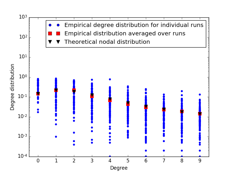
(a) $n=10000$, $R=100$

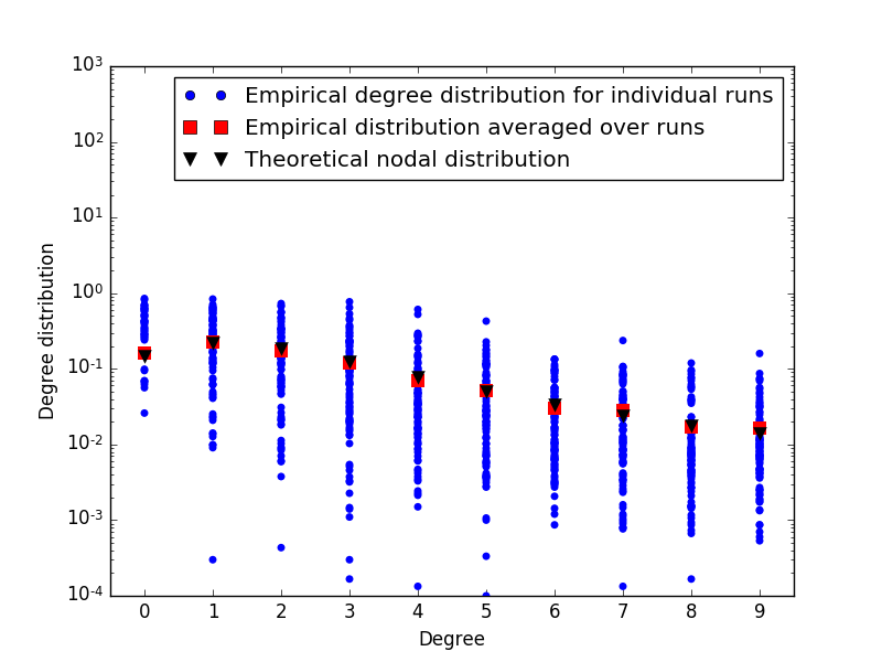
(b) $n=30000$, $R=100$

Figure 1:

We explore the behavior of the empirical degree distribution along the scaling (38) (with $\lambda=1$) as generated through a single network realization. We do so by plotting the histograms

$$\frac{N_{n}^{(r)}(d;\theta_{n}^{\star})}{n}=\frac{1}{n}\sum_{k=1}^{n}{\bf 1}\left[D^{(r)}_{n,k}(\theta^{\star}_{n})=d\right],\quad\begin{array}[]{c}d=0,1,\ldots\\ r=1,\ldots,R\\ \end{array}$$ (44)

for various values of $d$ and $r$, and large $n$, and comparing against the corresponding value for the limiting nodal distribution $p_{\rm Fuj}(d)$ given in (39). Using this expression we numerically evaluate $p_{\rm Fuj}(d)$ as

$$p_{\rm Fuj}(d)=\frac{1}{d!}\int_{0}^{\infty}\frac{e^{dx}}{d!}e^{-e^{x}}e^{-x}dx$$

for each $d=0,1,\ldots$. In Figure 1 we plot the histogram $\frac{N_{n}^{(r)}(.;\theta_{n}^{\star})}{n}$ for different runs $r=1,2,\ldots,R$ and varying graph sizes $n=10000,30000$. Observe the high variability with respect to the nodal degree distribution ${\mbox{\boldmath{$p$}}}_{\rm Fuj}$ which does not change as the graph size is increased.

We smooth out the variability observed in Figure 1 by averaging the empirical degree distributions (44) over the $R$ i.i.d. realizations $\mathbb{T}^{(1)}(n;\theta^{\star}_{n}),\mathbb{T}^{(2)}(n;\theta^{\star}_{n}),\ldots,\mathbb{T}^{(R)}(n;\theta^{\star}_{n})$. This results in the statistic

$$\frac{1}{R}\sum_{r=1}^{R}\frac{N_{n}^{(r)}(d;\theta_{n}^{\star})}{n},\ d=0,1,\ldots.$$ (45)

Fix $d=0,1,\ldots$. The Strong Law of Large Numbers yields

$$\lim_{R\rightarrow\infty}\frac{1}{R}\sum_{r=1}^{R}\frac{N_{n}^{(r)}(d;\theta_{n}^{\star})}{n}={\mathbb{E}}\left[{\frac{N_{n}(d;\theta_{n}^{\star})}{n}}\right]\quad\mbox{a.s.}$$ (46)

with

$${\mathbb{E}}\left[{\frac{N_{n}(d;\theta_{n}^{\star})}{n}}\right]={\mathbb{P}}\left[{D_{n,1}(\theta^{\star}_{n})=d}\right]$$

by exchangeability. On the other hand, by virtue of (40) we have $\lim_{n\rightarrow\infty}{\mathbb{P}}\left[{D_{n,1}(\theta^{\star}_{n})=d}\right]=p_{\rm Fuj}(d)$. Combining these observations yields the approximation

$$\frac{1}{R}\sum_{r=1}^{R}\frac{N_{n}^{(r)}(d;\theta_{n}^{\star})}{n}=_{\rm Approx}p_{\rm Fuj}(d)$$ (47)

for large $n$ and $R$. The goodness of the approximation (47) is noted in Figure 1, where the empirical distribution averaged over $R=100$ runs is observed to be very close to the nodal degree distribution. However, the accuracy of the approximation (47) does in no way imply the validity of (16). In fact the mistaken belief that (16) holds, implicitly assumed in the papers [13, 39], might have stemmed from using the smoothed estimate (47).

10 Preparing the proof of Proposition 8.1

For every $n=2,3,\ldots$ and $\theta>0$, the decomposition

$$D_{n,j}(\theta)={\bf 1}\left[\xi_{1}+\xi_{2}>\theta\right]+D^{\star}_{n,j}(\theta),\quad j=1,2$$ (48)

holds where we have set

$$D^{\star}_{n,j}(\theta)=\sum_{k=3}^{n}{\bf 1}\left[\xi_{j}+\xi_{k}>\theta\right].$$

Fix $d=0,1,\ldots$. It is a simple matter to check that

$$\left|{\mathbb{P}}\left[{D_{n,j}(\theta)=d}\right]-{\mathbb{P}}\left[{D^{\star}_{n,j}(\theta)=d}\right]\right|$$ (49)

$$\leq 2{\mathbb{P}}\left[{\xi_{1}+\xi_{2}>\theta}\right],\quad j=1,2$$

and

$$\left|{\mathbb{P}}\left[{D_{n,j}(\theta)=d,\ j=1,2}\right]-{\mathbb{P}}\left[{D^{\star}_{n,j}(\theta)=d,\ j=1,2}\right]\right|$$

$$\leq 2{\mathbb{P}}\left[{\xi_{1}+\xi_{2}>\theta}\right].$$ (50)

Next, for each $n=2,3,\ldots$ we substitute $\theta$ by $\theta^{\star}_{n}$ in the bound (50) and let $n$ go to infinity in the resulting inequality. Since $\lim_{n\rightarrow\infty}\theta^{\star}_{n}=\infty$, we conclude that $\lim_{n\rightarrow\infty}\big{|}{\mathbb{P}}\left[{D_{n,1}(\theta^{\star}_{n})=d,D_{n,2}(\theta^{\star}_{n})=d}\right]-{\mathbb{P}}\left[{D^{\star}_{n,1}(\theta^{\star}_{n})=d,D^{\star}_{n,2}(\theta^{\star}_{n})=d}\right]\big{|}=0$, whence

$$\lim_{n\rightarrow\infty}{\mathbb{P}}\left[{D_{n,1}(\theta^{\star}_{n})=d,D_{n,2}(\theta^{\star}_{n})=d}\right]$$ (51)

$$= \lim_{n\rightarrow\infty}{\mathbb{P}}\left[{D^{\star}_{n,1}(\theta^{\star}_{n})=d,D^{\star}_{n,2}(\theta^{\star}_{n})=d}\right]$$

provided either limit exists. The same argument applied to the bounds (49) readily yields

$$\lim_{n\rightarrow\infty}{\mathbb{P}}\left[{D_{n,j}(\theta^{\star}_{n})=d}\right] =\lim_{n\rightarrow\infty}{\mathbb{P}}\left[{D^{\star}_{n,j}(\theta^{\star}_{n})=d}\right]$$

$$=p_{\rm Fuj}(d),\quad j=1,2$$ (52)

in light of (40). It then follows from (51) and (52) that

$$C(d)$$

$$= \lim_{n\rightarrow\infty}{\rm Cov}\left[{\bf 1}\left[D^{\star}_{n,1}(\theta^{\star}_{n})=d\right],{\bf 1}\left[D^{\star}_{n,2}(\theta^{\star}_{n})=d\right]\right]$$

provided either limit at (51) exists.

As we now turn to evaluating (LABEL:eq:LimitGivesC(d)), it will be notationally convenient to introduce a second collection of $\mathbb{R}_{+}$-valued rvs $\{\eta_{\ell},\ \ell=1,2,\ldots\}$. We assume that the rvs $\{\eta_{\ell},\ \ell=1,2,\ldots\}$ are also i.i.d. rvs, each of which is exponentially distributed with parameter $\lambda>0$. The two collections $\{\xi,\xi_{k},\ k=1,2,\ldots\}$ and $\{\eta_{\ell},\ \ell=1,2,\ldots\}$ are assumed to be mutually independent. For each integer $p=2,3,\ldots$, let $\eta_{p|1},\ldots,\eta_{p|p}$ denote the values of the rvs $\eta_{1},\ldots,\eta_{p}$ arranged in decreasing order, namely $\eta_{p|p}\leq\ldots\leq\eta_{p|1}$, with a lexicographic tiebreaker when needed. The rvs $\eta_{p|1},\ldots,\eta_{p|p}$ are the order statistics associated with the collection $\eta_{1},\ldots,\eta_{p}$, so that for each $s=1,\ldots,p$, the rv $\eta_{p|s}$ denotes the $s^{th}$ largest value amongst $\eta_{1},\ldots,\eta_{p}$; in particular $\eta_{p|1}$ and $\eta_{p|p}$ are the maximum and minimum of the rvs $\eta_{1},\ldots,\eta_{p}$, respectively [17, 21].

The evaluation of the limiting covariances (LABEL:eq:LimitGivesC(d)) proceeds with the following observation: Fix $d=0,1,\ldots$ and take $n=3,4,\ldots$ such that $d\leq n-2$. Under the enforced i.i.d. assumptions, for each $\theta>0$ we get

$$\left(D^{\star}_{n,1}(\theta),D^{\star}_{n,2}(\theta)\right)$$

$$= \left(\sum_{k=3}^{n}{\bf 1}\left[\xi_{1}+\xi_{k}>\theta\right],\sum_{k=3}^{n}{\bf 1}\left[\xi_{2}+\xi_{k}>\theta\right]\right)$$

$$=_{st} \left(\sum_{\ell=1}^{n-2}{\bf 1}\left[\xi_{1}+\eta_{\ell}>\theta\right],\sum_{\ell=1}^{n-2}{\bf 1}\left[\xi_{2}+\eta_{\ell}>\theta\right]\right)$$

$$= \left(\sum_{\ell=1}^{n-2}{\bf 1}\left[\xi_{1}+\eta_{n-2|\ell}>\theta\right],\sum_{\ell=1}^{n-2}{\bf 1}\left[\xi_{2}+\eta_{n-2|\ell}>\theta\right]\right)$$

where $=_{st}$ denotes distributional equality between rvs. Two different cases arise:

First, with $d=0$ we find

$${\mathbb{P}}\left[{D^{\star}_{n,1}(\theta)=0}\right] = {\mathbb{P}}\left[{\sum_{\ell=1}^{n-2}{\bf 1}\left[\xi_{1}+\eta_{n-2|\ell}>\theta\right]=0}\right]$$ (54)

$$= {\mathbb{P}}\left[{\xi_{1}+\eta_{\ell}\leq\theta,\ \ell=1,\ldots,n-2}\right]$$

$$= {\mathbb{P}}\left[{\xi_{1}+\eta_{n-2|1}\leq\theta}\right]$$

$$= {\mathbb{P}}\left[{\eta_{n-2|1}-\theta\leq-\xi_{1}}\right]$$

and

$${\mathbb{P}}\left[{D^{\star}_{n,1}(\theta)=0,D^{\star}_{n,2}(\theta)=0}\right]$$ (55)

$$= {\mathbb{P}}\left[{\sum_{\ell=1}^{n-2}{\bf 1}\left[\xi_{j}+\eta_{n-2|\ell}>\theta\right]=0,\ j=1,2}\right]$$

$$= {\mathbb{P}}\left[{\xi_{1}+\eta_{\ell}\leq\theta,\xi_{2}+\eta_{\ell}\leq\theta,\ \ell=1,\ldots,n-2}\right]$$

$$= {\mathbb{P}}\left[{\xi_{1}+\eta_{n-2|1}\leq\theta,\xi_{2}+\eta_{n-2|1}\leq\theta}\right]$$

$$= {\mathbb{P}}\left[{\eta_{n-2|1}-\theta\leq-\max\left(\xi_{1},\xi_{2}\right)}\right].$$

Next we consider the case $d=1,2,\ldots$. Under the enforced independence assumptions we have

$${\mathbb{P}}\left[{D^{\star}_{n,1}(\theta)=d}\right]$$ (56)

$$= {\mathbb{P}}\left[{\sum_{\ell=1}^{n-2}{\bf 1}\left[\xi_{1}+\eta_{n-2|\ell}>\theta\right]=d}\right]$$

$$= {\mathbb{P}}\left[{\xi_{1}+\eta_{n-2|d+1}\leq\theta<\xi_{1}+\eta_{n-2|d}}\right]$$

$$= {\mathbb{P}}\left[{\theta-\eta_{n-2|d}<\xi_{1}\leq\theta-\eta_{n-2|d+1}}\right]$$

$$= {\mathbb{E}}\left[{e^{-\lambda(\theta-\eta_{n-2|d})^{+}}-e^{-\lambda(\theta-\eta_{n-2|d+1})^{+}}}\right]\hskip 28.45274pt$$

and

$${\mathbb{P}}\left[{D^{\star}_{n,1}(\theta)=d,D^{\star}_{n,2}(\theta)=d}\right]$$ (57)

$$= {\mathbb{P}}\left[{\sum_{\ell=1}^{n-2}{\bf 1}\left[\xi_{j}+\eta_{n-2|\ell}>\theta\right]=0,\ j=1,2}\right]$$

$$= {\mathbb{P}}\left[{\xi_{j}+\eta_{n-2|d+1}\leq\theta<\xi_{j}+\eta_{n-2|d},\ j=1,2}\right]$$

$$= {\mathbb{P}}\left[{\theta-\eta_{n-2|d}<\xi_{j}\leq\theta-\eta_{n-2|d+1},\ j=1,2}\right]$$

$$= {\mathbb{E}}\left[{\left(e^{-\lambda(\theta-\eta_{n-2|d})^{+}}-e^{-\lambda(\theta-\eta_{n-2|d+1})^{+}}\right)^{2}}\right].$$

In the next step, carried out in Section 12, we replace $\theta$ by $\theta^{\star}_{n}$ in the expressions above, and let $n$ go to infinity in the resulting expressions. To evaluate these limits we shall rely on asymptotic properties of the order statistics which are discussed next.

11 Asymptotic results for order statistics

We begin with a one-dimensional result. For each $s=1,2,\ldots$, consider the mapping $G_{s}:\mathbb{R}\rightarrow\mathbb{R}_{+}$ defined by

$$G_{s}(x_{s})\equiv\left(\sum_{m=0}^{s-1}\frac{e^{-mx_{s}}}{m!}\right)G(x_{s}),\quad x_{s}\in\mathbb{R}$$ (58)

where $G:\mathbb{R}\rightarrow\mathbb{R}_{+}$ denotes the well-known Gumbel distribution given by

$$G(x)=e^{-e^{-x}},\quad x\in\mathbb{R}.$$ (59)

The next result is well known [28, Thm. 2.2.1, p. 33], and takes the following form when applied to exponential distributions.

Lemma 11.1.

For each $s=1,2,\ldots$, it holds that

$$\lim_{p\rightarrow\infty}{\mathbb{P}}\left[{\lambda\left(\eta_{p|s}-\theta^{\star}_{p}\right)\leq x_{s}}\right]=G_{s}(x_{s}),\quad x_{s}\in\mathbb{R}$$ (60)

where the scaling $\theta^{\star}:\mathbb{N}_{0}\rightarrow\mathbb{R}$ is given by (38).

With $s=1$, Lemma 11.1 expresses the well-known membership of exponential distributions in the maximal domain of attraction of the Gumbel distribution [21] [28, Example 1.7.2, p. 21].

We now turn to the two-dimensional result we need: For each $s=1,2,\ldots$, define the mapping $J_{s}:\mathbb{R}^{2}\rightarrow\mathbb{R}_{+}$ given by

$$J_{s}(x_{s+1},x_{s})\equiv\sum_{k_{s}=0}^{s-1}\left(\ldots\right)\times\frac{e^{-k_{s}x_{s}}}{k_{s}!}\cdot e^{-e^{-\min(x_{s},x_{s+1})}}$$ (61)

with

$$\ldots=\sum_{k_{s+1}=k_{s}}^{s}\frac{\left(e^{-\min(x_{s},x_{s+1})}-e^{-x_{s}}\right)^{k_{s+1}-k_{s}}}{(k_{s+1}-k_{s})!}$$ (62)

as $x_{s}$ and $x_{s+1}$ range over $\mathbb{R}$. In these expressions we use the convention $0^{0}=1$.

Lemma 11.2.

For each $s=1,2,\ldots$, we have

$$\lim_{p\rightarrow\infty}{\mathbb{P}}\left[{\lambda(\eta_{p|s+1}-\theta^{\star}_{p})\leq x_{s+1},\lambda(\eta_{p|s}-\theta^{\star}_{p})\leq x_{s}}\right]$$ (63)

$$= J_{s}(x_{s+1},x_{s}),\quad x_{s+1},x_{s}\in\mathbb{R}$$

with mapping $J_{s}:\mathbb{R}^{2}\rightarrow\mathbb{R}_{+}$ given by (61)-(62), and scaling $\theta^{\star}:\mathbb{N}_{0}\rightarrow\mathbb{R}$ given by (38).

This result is a consequence of Theorem 2.3.1 in [28, p. 34]. As only the case $s=1$ was discussed in [28, Thm 2.3.2, p. 34], we provide in Section 13 a proof for arbitrary values of $s$ when the variates $\{\eta_{k},\ k=1,2,\ldots\}$ are exponentially distributed. By inspection we note from (61)-(62) that

$$J_{s}(x_{s+1},x_{s})=G_{s}(x_{s}),\quad\begin{array}[]{c}x_{s}\leq x_{s+1}\\ x_{s},x_{s+1}\in\mathbb{R}\\ \end{array}$$ (64)

so that

$$J_{s}(\infty,x_{s}) =\lim_{x_{s+1}\rightarrow\infty}J_{s}(x_{s+1},x_{s})$$

$$=G_{s}(x_{s}),\quad x_{s}\in\mathbb{R}$$ (65)

while

$$J_{s}(x_{s+1},\infty) =\lim_{x_{s}\rightarrow\infty}J_{s}(x_{s+1},x_{s})$$

$$=G_{s+1}(x_{s+1}),\quad x_{s+1}\in\mathbb{R}.$$ (66)

This confirms that the probability distributions $G_{s+1}$ and $G_{s}$ are the one-dimensional marginal distributions of $J_{s}$ (as expected).

For use in Section 12 we find it convenient to give Lemma 11.1 and Lemma 11.2 the following probabilistic (and more compact) formulation: For any given $s=1,2,\ldots$, there exists a pair of $\mathbb{R}$-valued rvs $\Lambda_{s+1}$ and $\Lambda_{s}$ defined on $(\Omega,\mathcal{F},\mathbb{P})$ such that

$$\lambda\left(\eta_{p|s+j}-\theta^{\star}_{p}\right)\Longrightarrow_{p}\Lambda_{s+j},\quad j=0,1$$ (67)

and

$$\left(\lambda\left(\eta_{p|s+1}-\theta^{\star}_{p}\right),\lambda\left(\eta_{p|s}-\theta^{\star}_{p}\right)\right)\Longrightarrow_{p}(\Lambda_{s+1},\Lambda_{s})$$ (68)

with $(\Lambda_{s+1},\Lambda_{s})$ jointly distributed according to $J_{s}$, and the $\mathbb{R}$-valued rvs $\Lambda_{s+1}$ and $\Lambda_{s}$ distributed according to $G_{s+1}$ and $G_{s}$, respectively.

12 Completing the proof of Proposition 8.1

We return to the expressions obtained in Section 10: With $d=0,1,\ldots$ held fixed, for each $n=2,3,\ldots$ we substitute $\theta$ by $\theta^{\star}_{n}$ in these expressions according to (38), and let $n$ go to infinity in the resulting expressions.

12.1 The case $d=0$

For each $n=3,4,\ldots$, with the aforementioned substitution, we rewrite (54) and (55) as

$${\mathbb{P}}\left[{D^{\star}_{n,1}(\theta^{\star}_{n})=0}\right]={\mathbb{P}}\left[{\lambda(\eta_{n-2|1}-\theta^{\star}_{n})\leq-\lambda\xi_{1}}\right]$$

and

$${\mathbb{P}}\left[{D^{\star}_{n,1}(\theta^{\star}_{n})=0,D^{\star}_{n,2}(\theta^{\star}_{n})=0}\right]$$

$$= {\mathbb{P}}\left[{\lambda(\eta_{n-2|1}-\theta^{\star}_{n})\leq-\lambda\max(\xi_{1},\xi_{2})}\right]$$

where by construction the rv $\eta_{n-2|1}$ is independent of the i.i.d. rvs $\xi_{1}$ and $\xi_{2}$.

Let $\Lambda_{1}$ denote a rv which is distributed according to the Gumbel distribution (59), and which is independent of the i.i.d. rvs $\xi_{1}$ and $\xi_{2}$. By Lemma 11.1 (for $s=1$ and $p=n-2$), since $\lim_{n\rightarrow\infty}\left(\theta^{\star}_{n}-\theta^{\star}_{n-2}\right)=0$, it is now plain that

$$p_{\rm Fuj}(0) = \lim_{n\rightarrow\infty}{\mathbb{P}}\left[{D^{\star}_{n,1}(\theta^{\star}_{n})=0}\right]$$

$$= {\mathbb{P}}\left[{\Lambda_{1}\leq-\lambda\xi_{1}}\right]={\mathbb{E}}\left[{e^{-e^{\lambda\xi_{1}}}}\right]$$

and

$$\lim_{n\rightarrow\infty}{\mathbb{P}}\left[{D^{\star}_{n,1}(\theta^{\star}_{n})=0,D^{\star}_{n,2}(\theta^{\star}_{n})=0}\right]$$

$$= {\mathbb{P}}\left[{\Lambda_{1}\leq-\lambda\max(\xi_{1},\xi_{2})}\right]={\mathbb{E}}\left[{e^{-e^{\lambda\max(\xi_{1},\xi_{2})}}}\right]$$

under the independence assumptions. Collecting these facts, we find

$$\lim_{n\rightarrow\infty}{\rm Cov}\left[{\bf 1}\left[D^{\star}_{n,1}(\theta^{\star}_{n})=0\right],{\bf 1}\left[D^{\star}_{n,2}(\theta^{\star}_{n})=0\right]\right]$$ (69)

$$= {\mathbb{E}}\left[{e^{-e^{\lambda\max(\xi_{1},\xi_{2})}}}\right]-{\mathbb{E}}\left[{e^{-e^{\lambda\xi_{1}}}}\right]{\mathbb{E}}\left[{e^{-e^{\lambda\xi_{2}}}}\right].$$

As we make use of the reduction step (LABEL:eq:LimitGivesC(d)) discussed in Section 10. It follows that

$$C(0) = \lim_{n\rightarrow\infty}{\rm Cov}\left[{\bf 1}\left[D^{\star}_{n,1}(\theta^{\star}_{n})=0\right],{\bf 1}\left[D^{\star}_{n,2}(\theta^{\star}_{n})=0\right]\right]$$ (70)

$$= {\mathbb{E}}\left[{e^{-e^{\lambda\max(\xi_{1},\xi_{2})}}}\right]-{\mathbb{E}}\left[{e^{-e^{\lambda\xi_{1}}}}\right]{\mathbb{E}}\left[{e^{-e^{\lambda\xi_{2}}}}\right]$$

$$> 0$$

since $\max(e^{\lambda\xi_{1}},e^{\lambda\xi_{2}})<e^{\lambda\xi_{1}}+e^{\lambda\xi_{2}}$.  

12.2 The case $d=1,2,\ldots$

Pick $n=3,4,\ldots$ such that $d<n-2$. Under the aforementioned substitution, we can rewrite (56) and (57) as

$${\mathbb{P}}\left[{D^{\star}_{n,1}(\theta^{\star}_{n})=d}\right]$$ (71)

$$= {\mathbb{E}}\left[{e^{-\lambda(\theta^{\star}_{n}-\eta_{n-2|d})^{+}}-e^{-\lambda(\theta^{\star}_{n}-\eta_{n-2|d+1})^{+}}}\right]$$

and

$${\mathbb{P}}\left[{D^{\star}_{n,1}(\theta^{\star}_{n})=d,D^{\star}_{n,2}(\theta^{\star}_{n})=d}\right]$$ (72)

$$= {\mathbb{E}}\left[{\left(e^{-\lambda(\theta^{\star}_{n}-\eta_{n-2|d})^{+}}-e^{-\lambda(\theta^{\star}_{n}-\eta_{n-2|d+1})^{+}}\right)^{2}}\right].$$

Applying Lemma 11.1 and Lemma 11.2 (for $s=d$ and $p=n-2$) we conclude that

$$\left(\lambda\left(\eta_{n-2|d+1}-\theta^{\star}_{n-2}\right),\lambda\left(\eta_{n-2|d}-\theta^{\star}_{n-2}\right)\right)\Longrightarrow_{n}(\Lambda_{d+1},\Lambda_{d})$$

in the notation used at (68). Because $\lim_{n\rightarrow\infty}\left(\theta^{\star}_{n}-\theta^{\star}_{n-2}\right)=0$, we obtain

$$\left(\lambda\left(\theta^{\star}_{n}-\eta_{n-2|d+1}\right)^{+},\lambda\left(\theta^{\star}_{n}-\eta_{n-2|d}\right)^{+}\right)$$

$$\Longrightarrow_{n}((-\Lambda_{d+1})^{+},(-\Lambda_{d})^{+})\hskip 91.04881pt$$

by the Continuous Mapping Theorem for weak convergence, whence

$$e^{-\lambda(\theta^{\star}_{n}-\eta_{n-2|d})^{+}}-e^{-\lambda(\theta^{\star}_{n}-\eta_{n-2|d+1})^{+}}$$

$$\Longrightarrow_{n}e^{-(-\Lambda_{d})^{+}}-e^{-(-\Lambda_{d+1})^{+}}$$

by applying the Continuous Mapping Theorem once more.

Let $n$ go to infinity in (71) and (72): The Bounded Convergence Theorem yields

$$\lim_{n\rightarrow\infty}{\mathbb{E}}\left[{\left(e^{-\lambda(\theta^{\star}_{n}-\eta_{n-2|d})^{+}}-e^{-\lambda(\theta^{\star}_{n}-\eta_{n-2|d+1})^{+}}\right)^{a}}\right]$$ (73)

$$= {\mathbb{E}}\left[{\left(e^{-(-\Lambda_{d})^{+}}-e^{-(-\Lambda_{d+1})^{+}}\right)^{a}}\right]\hskip 56.9055pt$$

for each $a=1,2$ upon observing the obvious bounds

$$\left|e^{-\lambda(\theta^{\star}_{n}-\eta_{n-2|d})^{+}}-e^{-\lambda(\theta^{\star}_{n}-\eta_{n-2|d+1})^{+}}\right|\leq 1,\quad n=3,4,\ldots$$

It follows that

$$\lim_{n\rightarrow\infty}{\rm Cov}\left[{\bf 1}\left[D^{\star}_{n,1}(\theta^{\star}_{n})=d\right],{\bf 1}\left[D^{\star}_{n,2}(\theta^{\star}_{n})=d\right]\right]$$

$$= {\mathbb{E}}\left[{\left(e^{-(-\Lambda_{d})^{+}}-e^{-(-\Lambda_{d+1})^{+}}\right)^{2}}\right]$$

$$-\left({\mathbb{E}}\left[{e^{-(-\Lambda_{d})^{+}}-e^{-(-\Lambda_{d+1})^{+}}}\right]\right)^{2}\hskip 42.67912pt$$

and the reduction step (LABEL:eq:LimitGivesC(d)) leads to

$$C(d) = \lim_{n\rightarrow\infty}{\rm Cov}\left[{\bf 1}\left[D^{\star}_{n,1}(\theta^{\star}_{n})=d\right],{\bf 1}\left[D^{\star}_{n,2}(\theta^{\star}_{n})=d\right]\right]$$ (74)

$$= {\rm Var}\left[e^{-(-\Lambda_{d})^{+}}-e^{-(-\Lambda_{d+1})^{+}}\right].$$

Note that $C(d)>0$ as the variance of the non-degenerate rv $e^{-(-\Lambda_{d})^{+}}-e^{-(-\Lambda_{d+1})^{+}}$.  

13 A Proof of Lemma 11.2

First some preliminaries. Fix $p=1,2,\ldots$ and $u\geq 0$. The rv $S_{p}(u)$ given by

$$S_{p}(u)=\sum_{\ell=1}^{p}{\bf 1}\left[\xi_{\ell}>u\right]$$

counts the number of exceedances of level $u$ by the rvs $\xi_{1},\ldots,\xi_{p}$. The proof of Lemma 11.2 relies on the well-known equivalence

$$\eta_{p|s}\leq u\quad\mbox{if and only if}\quad S_{p}(u)<s,\quad s=0,1,\ldots,p$$ (75)

given in [28, Section 2.2, p. 33]; see also [28, Theorem 2.3.2, p. 36] for the case $s=1$. Throughout we shall write

$$u_{p}(x)=\lambda^{-1}\left(\log p+x\right)^{+},\quad x\in\mathbb{R}.$$ (76)

Fix $s=1,2,\ldots$, and pick $x_{s}$ and $x_{s+1}$ in $\mathbb{R}$. Two cases are possible:

(i) If $x_{s}\leq x_{s+1}$ in $\mathbb{R}$, then for each $p=s+1,s+2,\ldots$, it holds that $u_{p}(x_{s})\leq u_{p}(x_{s+1})$, whence

$${\mathbb{P}}\left[{\eta_{p|s+1}\leq u_{p}(x_{s+1}),\eta_{p|s}\leq u_{p}(x_{s})}\right]$$

$$= {\mathbb{P}}\left[{\eta_{p|s+1}\leq u_{p}(x_{s}),\eta_{p|s}\leq u_{p}(x_{s})}\right]$$

$$= {\mathbb{P}}\left[{\eta_{p|s}\leq u_{p}(x_{s})}\right]$$

since $\eta_{p|s+1}\leq\eta_{p|s}$. From Lemma 11.1 it follows that

$$\lim_{p\rightarrow\infty}{\mathbb{P}}\left[{\lambda(\eta_{p|s+1}-\theta^{\star}_{p})\leq x_{s+1},\lambda(\eta_{p|s}-\theta^{\star}_{p})\leq x_{s}}\right]$$

$$= \lim_{p\rightarrow\infty}{\mathbb{P}}\left[{\lambda(\eta_{p|s}-\theta^{\star}_{p})\leq x_{s}}\right]$$

$$= G_{s}(x_{s})$$

and (63) holds as seen through (64).

(ii) If $x_{s+1}\leq x_{s}$ in $\mathbb{R}$, then for each $p=s+1,s+2,\ldots$, the equivalence (75) yields

$${\mathbb{P}}\left[{\eta_{p|s+1}\leq u_{p}(x_{s+1}),\eta_{p|s}\leq u_{p}(x_{s})}\right]$$ (77)

$$= {\mathbb{P}}\left[{S_{p}(u_{p}(x_{s+1}))<s+1,S_{p}(u_{p}(x_{s}))<s}\right]$$

$$= \sum_{k_{s}=0}^{s-1}\left(\sum_{k_{s+1}=0}^{s}{\mathbb{P}}\left[{\begin{array}[]{c}S_{p}(u_{p}(x_{s+1}))=k_{s+1}\\ \\ S_{p}(u_{p}(x_{s}))=k_{s}\\ \end{array}}\right]\right)$$ (81)

$$= \sum_{k_{s}=0}^{s-1}\Bigg{(}\sum_{k_{s+1}=k_{s}}^{s}{\mathbb{P}}\left[{\begin{array}[]{c}\sum_{\ell=1}^{p}{\bf 1}\left[\xi_{\ell}>u_{p}(x_{s+1})\right]=k_{s+1}\\ \\ \sum_{\ell=1}^{p}{\bf 1}\left[\xi_{\ell}>u_{p}(x_{s})\right]=k_{s}\end{array}}\right]$$ (85)

upon noting the fact $S_{p}(u_{p}(x_{s}))\leq S_{p}(u_{p}(x_{s+1}))$ since $u_{p}(x_{s+1})\leq u_{p}(x_{s})$. For arbitrary $k_{s},k_{s+1}=0,1,\ldots$ with $k_{s}\leq k_{s+1}$, standard counting arguments give

$${\mathbb{P}}\left[{\begin{array}[]{c}\sum_{\ell=1}^{p}{\bf 1}\left[\xi_{\ell}>u_{p}(x_{s+1})\right]=k_{s+1}\\ \\ \sum_{\ell=1}^{p}{\bf 1}\left[\xi_{\ell}>u_{p}(x_{s})\right]=k_{s}\end{array}}\right]$$ (90)

$$= {p\choose k_{s}}e^{-\lambda k_{s}u_{p}(x_{s})}\left(e^{-\lambda u_{p}(x_{s+1})}-e^{-\lambda u_{p}(x_{s})}\right)^{k_{s+1}-k_{s}}$$

$$\times{p-k_{s}\choose k_{s+1}-k_{s}}\left(1-e^{-\lambda u_{p}(x_{s+1})}\right)^{p-k_{s+1}}$$

$$= \frac{1}{k_{s}!(k_{s+1}-k_{s})!}\cdot\frac{p!\cdot p^{-k_{s+1}}}{(p-k_{s+1})!}\cdot e^{-k_{s}x_{s}}$$

$$\times\left(e^{-x_{s+1}}-e^{-x_{s}}\right)^{k_{s+1}-k_{s}}\cdot\left(1-\frac{e^{-x_{s+1}}}{p}\right)^{p-k_{s+1}}$$

where the last step holds whenever $p$ is large enough so that $\log p+x_{s}>0$ and $\log p+x_{s+1}>0$.

Let $p$ go to infinity in (81): From (90) the limit of each term in (81) is given by

$$\lim_{p\rightarrow\infty}{\mathbb{P}}\left[{\begin{array}[]{c}\sum_{\ell=1}^{p}{\bf 1}\left[\xi_{\ell}>u_{p}(x_{s+1})\right]=k_{s+1}\\ \\ \sum_{\ell=1}^{p}{\bf 1}\left[\xi_{\ell}>u_{p}(x_{s})\right]=k_{s}\\ \end{array}}\right]$$

$$= \frac{e^{-k_{s}x_{s}}}{k_{s}!}\cdot\frac{\left(e^{-x_{s+1}}-e^{-x_{s}}\right)^{k_{s+1}-k_{s}}}{(k_{s+1}-k_{s})!}\cdot e^{-e^{-x_{s+1}}}$$

for $k_{s}\leq k_{s+1}$ in $\mathbb{N}$, as we note that

$$\lim_{p\rightarrow\infty}\frac{p!}{(p-k_{s+1})!\cdot p^{k_{s+1}}}=1$$

and

$$\lim_{p\rightarrow\infty}\left(1-\frac{e^{-x_{s+1}}}{p}\right)^{p-k_{s+1}}=e^{-e^{-x_{s+1}}}.$$

The convergence (63) follows upon using the equivalence (77) together with the observation that $u_{p}(x_{s})=\lambda^{-1}\left(\log p+x_{s}\right)$ and $u_{p}(x_{s+1})=\lambda^{-1}\left(\log p+x_{s+1}\right)$ for $p$ sufficiently large.  

Siddharth Pal received his Bachelors degree in Electronics and Telecommunication Engineering from Jadavpur University, India, in 2011, and his Masters and Ph.D degrees. both in Electrical Engineering from University of Maryland College Park, USA, in 2014 and 2015 respectively. Since then he has been working as a research scientist at Raytheon BBN Technologies. His research interests include network science and analysis, game theory, machine learning with emphasis on neural network based approaches, and stochastic systems.

Armand M. Makowski (M’83√±-SM’94√±-F’06) received the Licence en Sciences Mathématiques from the Université Libre de Bruxelles in 1975, the M.S. degree in Engineering-Systems Science from U.C.L.A. in 1976 and the Ph.D. degree in Applied Mathematics from the University of Kentucky in 1981. In August 1981, he joined the faculty of the Electrical Engineering Department at the University of Maryland College Park, where he is Professor of Electrical and Computer Engineering. He has held a joint appointment with the Institute for Systems Research since its establishment in 1985. Armand Makowski was a C.R.B. Fellow of the Belgian-American Educational Foundation (BAEF) for the academic year 1975-76; he is also a 1984 recipient of the NSF Presidential Young Investigator Award and became an IEEE Fellow in 2006. His research interests lie in applying advanced methods from the theory of stochastic processes to the modeling, design and performance evaluation of engineering systems, with particular emphasis on communication systems and networks.

References

- [1] R. Albert and A.L. Barabási, “Statistical mechanics of complex systems,” Review of Modern Physics 74 (2002), pp. 47-97.
- [2] D. Aldous and J.M. Steele, “The Objective Method: Probabilistic Combinatorial Optimization and Local Weak Convergence,” Probability on Discrete Structures pp. 1-72
- [3] A.L. Barabási and R. Albert, “Emergence of scaling in random networks,” Science 286 (1999), pp. 509-512.
- [4] A. Barrat, M. Barthélemy and A. Vespignani, Dynamical Processes on Complex Networks, Cambridge University Press, Cambridge (U.K.), 2008.
- [5] I. Benjamini and O. Schramm, “Recurrence of distributional limits of finite planar graphs,” Electronic Journal of Probability 6 (2001), pp. 1-13.
- [6] N. Berger, C. Borgs, J.T. Chayes and A. Saberi, “Asymptotic behavior and distributional limits of preferential attachment graphs,” The Annals of Probability 42 (20140, pp. 1-40.
- [7] P. Billingsley, Convergence of Probability Measures, John Wiley & Sons, New York (NY), 1968.
- [8] E.A. Bender and E.R. Caulfield, “The asymptotic number of labelled graphs with given degree sequence,” Journal of Combinatorial Theory (A) 24 (1978), pp. 296-307.
- [9] B. Bollobás, “A probabilistic proof of an asymptotic formula for the number of labelled regular graphs,” European Journal of Combinatorics 1 (1980), pp. 311-316.
- [10] B. Bollobás, Random Graphs, Second Edition, Cambridge Studies in Advanced Mathematics, Cambridge University Press, Cambridge (UK), 2001.
- [11] B. Bollobás, O. Riordan, J. Spencer and G. Tusnády, “The degree sequence of a scale free random graph process,” Random Structures and Algorithms 18 (2001), pp. 279-290.
- [12] T. Britton, M. Deijfen, and A. Martin-Löf, “Generating simple random graphs with prescribed degree distribution,” Journal of Statistical Physics 124 (2006), pp. 1377-1397.
- [13] G. Caldarelli, A. Capocci, P. De Los Rios and M.A. Muñoz, “Scale-free networks from varying vertex intrinsic fitness,” Physical Review Letters 89 (2002), 258702.
- [14] K.L. Chung, A Course in Probability Theory, Second Edition, Academic Press, Harcourt, New York (NY), 1974.
- [15] A. Clauset, C. Rohilla Shalizi and M.E.J. Newman, “Power-law distributions in empirical data,” SIAM Review 51 (2009), pp. 661-703.
- [16] R. Cohen and S. Havlin, Complex Networks: Structure, Robustness and Function, Cambridge University Press, Cambridge (U.K.), 2010.
- [17] H.A. David and H.N. Nagaraja, Order Statistics, 3rd Edition, Wiley Series in Probability and Statistics, John Wiley & Sons, Hoboken (NJ), 2003.
- [18] M. Draief and L. Massoulié, Epidemics and Rumours in Complex Networks, London Mathematical Society Lecture Note Series 369, Cambridge University Press, Cambridge (UK), 2010.
- [19] S.N. Dorogovstev and J.F.F. Mendes, “Evolution of networks,” Advances in Physics 51 (2002), pp. 1097-1187.
- [20] R. Durrett, Random Graph Dynamics, Cambridge Series in Statistical and Probabilistic Mathematics, Cambridge University Press, Cambridge (U.K.), 2007.
- [21] P. Embrechts, C. Klüppelberg and T. Mikosch, Modelling Extremal Events for Insurance and Finance, Stochastic Modelling and Applied Probability, Springer-Verlag, New York (NY), 1997.
- [22] P. Erdős and A. Rényi, “On the evolution of random graphs,” Publ. Math. Inst. Hung. Acad. Sci 5 (1960), pp. 17-61.
- [23] A. Fujihara, Y. Ide, N. Konno, N. Masuda, H. Miwa and M. Uchida, “Limit theorems for the average distance and the degree distribution of the threshold network model,” Interdisciplinary Information Sciences 15 (2003), pp. 361-366.
- [24] P.W. Holland and S. Leinhardt, “An exponential family of probability distributions for directed graphs,” Journal of the American Statistical Association 76 (1981), pp. 33-50.
- [25] M.O. Jackson, Social and Economic Networks, Princeton University Press, Princeton (NJ), 2008.
- [26] S. Janson, T. Łuczak and A. Ruciński, Random Graphs, Wiley-Interscience Series in Discrete Mathematics and Optimization, John Wiley & Sons, 2000.
- [27] M. Kim and J. Leskovec, “Multiplicative attribute graph model of real-world networks,” Internet Mathematics 8 (2011), pp. 113-160.
- [28] M.R. Leadbetter, G. Lindgren and H. Rootzén Extremes and Related Properties of Random Sequences and Processes, Springer Series in Statistics, Springer (Berlin), 1983.
- [29] A. M. Makowski and O. Yağan, “Scaling laws for connectivity in random threshold graph models with non-negative fitness variables,” IEEE Journal on Selected Areas in Communications JSAC–31 (2013), Special Issues on Emerging Technologies in Communications (Area 4: Social Networks).
- [30] M. Molloy and B. Reed, “A critical point for random graphs with a given degree sequence,” Random Structures and Algorithms 6 (1995), pp. 161-179.
- [31] M. Molloy and B. Reed, “The size of the giant component of a random graph with a given degree sequence,” Journal of Combinatorics, Probability and Computing 7 (1988), pp. 295-305
- [32] M.E.J. Newman, “The structure and function of complex networks,” SIAM Review 45 (2003), pp. 167-256.
- [33] M.E.J. Newman, Networks: An Introduction, Oxford University Press, Oxford (U.K.), 2010.
- [34] M.E.J. Newman, A.L. Barabási and D.J. Watts, Edrs., The Structure and Dynamics of Networks, Princeton University Press, Princeton (NJ), 2006.
- [35] S. Pal, Adventures on Networks: Degrees and Games, Ph.D. Thesis, Department of Electrical and Computer Engineering, University of Maryland, College Park (MD). December 2015.
- [36] S. Pal and A.M. Makowski, “On the asymptotics of degree distributions,” in the Proceedings of the 53rd IEEE Conference on Decision and Control (CDC 2015), Osaka (Japan), December 2015.
- [37] M.D. Penrose, Random Geometric Graphs, Oxford Studies in Probability 5, Oxford University Press, New York (NY), 2003.
- [38] S. Qu and A.M. Makowski, “On the log-normality of the degree distribution in large homogeneous binary multiplicative attribute graph models,” Available at arXiv:1810.10114.
- [39] V.D.P. Servedio and G. Caldarelli, “Vertex intrinsic fitness: How to produce arbitrary scale-free networks,” Physical Review E 70 (2004), 056126.
- [40] D. Strauss, “On a general class of models for interaction,” SIAM Review 28 (1986), pp. 513-527.
- [41] O. Yağan and A.M. Makowski, “Zero-one laws for connectivity in random key graphs.” IEEE Transactions on Information Theory IT-58 (2012), pp. 2983-2999.