Imposing jump conditions on nonconforming interfaces for the Correction Function Method: a least squares approach

Abstract

We introduce a technique that simplifies the problem of imposing jump conditions on interfaces that are not aligned with a computational grid in the context of the Correction Function Method (CFM). The CFM offers a general framework to solve Poisson’s equation in the presence of discontinuities to high order of accuracy, while using a compact discretization stencil. A key concept behind the CFM is enforcing the jump conditions in a least squares sense. This concept requires computing integrals over sections of the interface, which is a challenge in 3-D when only an implicit representation of the interface is available (e.g., the zero contour of a level set function). The technique introduced here is based on a new formulation of the least squares procedure that relies only on integrals over domains that are amenable to simple quadrature after local coordinate transformations. We incorporate this technique into a fourth order accurate implementation of the CFM, and show examples of solutions to Poisson’s equation computed in 2-D and 3-D.

1 Introduction

Solving Poisson’s equation in the presence of discontinuities is of great importance in science and engineering applications. In many cases, the discontinuities are caused by interfaces between different media, such as in multiphase flows, Stefan’s problem, Janus drops, and other multiphase phenomena. These interfaces follow themselves from solutions to differential equations, and can assume complex configurations. For this reason, it is convenient to embed the interface into a regular triangulation or Cartesian grid and solve Poisson’s equation in this regular domain. The Correction Function Method (CFM) [1, 2, 3] was developed to solve Poisson’s equation in this context, and achieve high order of accuracy with a compact discretization stencil.

The CFM is based on the concept of the correction function (introduced in §2.1), which is the minimizer of an energy functional constructed to impose the jump conditions and locally satisfy Poisson’s equation. In the present paper we leverage the flexibility in this construction and propose a new formulation that simplifies numerical implementation. A key ingredient of the CFM is computing integrals over sections of the interface, which is a challenge in 3-D when only an implicit representation of the interface is available (e.g., the zero contour of a level set function). There are several recent methods that focus specifically on integrating functions on implicitly defined surfaces [4, 5, 6, 7, 8]. However, these methods are designed to solve general problems that include non-trivial integration domains. In our context, we are free to define the energy functional and we use this flexibility to simplify the integration problem. Specifically, we define integration domains using approximate coordinate transformations such that we can always use standard quadrature techniques.

We now define the problem precisely. Poisson’s equation with imposed discontinuities (for brevity: discontinuous Poisson equation) is given by

$$\nabla\cdot\bigl{(}\beta(\vec{x})\nabla u(\vec{x})\bigr{)} =f(\vec{x}) \mathrm{for}\;\;\vec{x} \in\Omega\/,$$ (1a)

$$[u(\vec{x})] =a(\vec{x}) \mathrm{for}\;\;\vec{x} \in\Gamma\/,$$ (1b)

$$[\beta(\vec{x})u_{n}(\vec{x})] =b(\vec{x}) \mathrm{for}\;\;\vec{x} \in\Gamma\/,$$ (1c)

$$u(\vec{x}) =g(\vec{x}) \mathrm{for}\;\;\vec{x} \in\partial\Omega\/.$$ (1d)

Here the solution domain $\Omega\/$ is split into two sub-domains, $\Omega_{1}\/$ and $\Omega_{2}\/$, by a co-dimension 1 surface, $\Gamma\/$, disjoint from the boundary $\partial\Omega\/$. This situation is illustrated in figure 1. Furthermore, $a\/$ and $b\/$ are known functions defined on $\Gamma\/$, and square brackets denote the jump in the enclosed quantity across $\Gamma\/$, i.e.,

$$[u(\vec{x})]=\lim_{\begin{subarray}{c}\vec{x}^{\ast}\,\to\,\vec{x}\\ \vec{x}^{\ast}\,\in\,\Omega_{2}\end{subarray}}u(\vec{x}^{\ast})-\lim_{\begin{subarray}{c}\vec{x}^{\ast}\,\to\,\vec{x}\\ \vec{x}^{\ast}\,\in\,\Omega_{1}\end{subarray}}u(\vec{x}^{\ast})\/.$$

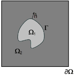
Figure 1: Illustration of the solution domain for the discontinuous Poisson equation. The domain $\Omega\/$ is split into two subdomains, $\Omega_{1}\/$ and $\Omega_{2}\/$, by the internal interface $\Gamma\/$.

In addition, we assume Dirichlet conditions on the domain boundary $\partial\Omega\/$, and that this boundary is aligned with the computational grid. However, other boundary conditions can be used, such as Neumann or Robin, with no effect on how jump conditions are imposed on the interface $\Gamma\/$.

Remark 1.

The coefficient $\beta\/$ denotes a known positive function, $\beta=\beta(\vec{x})$. In many applications, $\beta\/$ is discontinuous across the interface $\Gamma\/$. However, in this paper we only consider the case where $\beta\/$ is constant. The subject of this paper is imposing the jump conditions when only an implicit representation of the interface is available. The case of discontinuous $\beta\/$ introduces additional difficulties in the context of the CFM formulation that are not related to the subject of this paper. Hence, we address the matter of discontinuous $\beta\/$ in separate work. This matter was partially addressed in ref. [3] by coupling the CFM with boundary integral equations. However, solving boundary integral equations to high order of accuracy using level set functions is also a challenge. For this reason, work on a more general framework for the case of discontinuous $\beta\/$ is ongoing and will be addressed in future publications.

Over the past four decades, several methods have been developed to solve (1), and other closely related problems, with either an interface or a boundary that is embedded into a regular triangulation or Cartesian grid [9, 10, 11, 12, 13, 14, 15, 16, 17, 18, 19, 20, 21, 22, 23, 24, 25, 26, 27, 28, 29, 30, 31, 32, 33, 34, 35, 36, 37, 38]. One of the shortcomings of many embedded methods is that they are rather hard to generalize beyond first or second order of accuracy. However, there are methods that achieve accuracy higher than second order, based on one of the following ideas: (i) discretization stencils that incorporate the jump (or boundary) conditions [20, 21, 22, 27, 28], or (ii) smooth extrapolations of the solution constrained by the jump (or boundary) conditions [18, 32, 33, 34]. In practice these ideas are implemented by Taylor expansion or a similar concept, and high order of accuracy is obtained at the expense of wide discretization stencils. In turn, wide stencils introduce additional issues, such as handling multiple crossings of the interface by a single stencil, and restrictions on the proximity between interfaces. The method introduced by Mayo and collaborators [20, 21, 22] avoids wide discretization stencils by incorporating second and third derivatives of the jump conditions into the Taylor expansion. On the other hand, computing higher derivatives of the jump conditions requires the solution of an additional boundary integral equation.

In contrast to using Taylor expansion, the CFM [1, 2, 3] is based on computing a smooth extension of the solution by solving a partial differential equation that is compatible with Poisson’s equation. This concept results in a general framework that, in principle, can achieve arbitrary order of accuracy, and maintains compact discretization stencils. In ref. [1] we introduced the fundamentals of the CFM, and proposed a fourth order implementation to solve (1) in 2-D when $\beta\/$ is constant. In ref. [3] we extended the CFM to solve (1) with piece-wise constant $\beta\/$, including the possibility of arbitrarily large jumps in the equation’s coefficients (in [3] we showed third order convergence for coefficient ratios of $O(10^{6})$). The work of ref. [3] is inspired by Mayo’s method [20, 21], and also requires the solution of a boundary integral equation. However, there is an extension of the CFM for the case of discontinuous $\beta\/$ that does not require the solution of a boundary integral equation. This extension is briefly discussed in ref. [2], and is the subject of current research by the authors. The CFM has also been extended to other classes of differential equations, such as the heat equation [2], the Navier-Stokes equations [2], and the wave equation [39].

This paper is organized as follows. In §2 we present an overview of the CFM for Poisson’s equation. Next, in §3 we present the details of the new technique for imposing the jump conditions in a least squares sense, including its effects on the CFM formulation. In §4 we present solutions computed with the modified CFM in 2-D and 3-D. Finally, the conclusions are in §5.

2 Overview of the Correction Function Method

2.1 The correction function

The Correction Function Method (CFM) was developed to solve the discontinuous Poisson problem (1) when the interface $\Gamma\/$ is not aligned with a computational grid [1, 2, 3]. The CFM is based on the notion of smooth extensions of the solution (denoted by $u_{1}\/$ and $u_{2}\/$) across the interface, and the definition of the correction function: $D=u_{2}-u_{1}\/$. This function can be used to complete discretization stencils that stride the interface.

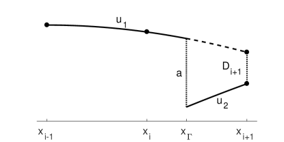
Figure 2: Illustration of how the correction function is used to complete discretization stencils. To compute $u_{xx_{i}}\/$, write $u_{1_{i+1}}=u_{2_{i+1}}-D_{i+1}\/$, which leads to (3).

We illustrate this point with a 1-D example. Consider the approximate computation of $u_{xx}\/$ at grid node $i\/$ using standard centered finite differences:

$$u_{xx_{i}}\approx\dfrac{u_{i-1}-2u_{i}+u_{i+1}}{h^{2}},$$ (2)

where $h\/$ is a uniform grid spacing. Equation (2) is known to produce errors $O(h^{2})\/$ if $u\in C^{2}((x_{i-1},x_{i+1}))\/$. However, when $u\/$ is discontinuous, as depicted in figure 2, the approximation in (2) is not valid since it is based on Taylor expansions. One way to address this issue, originally introduced in the Ghost Fluid Method [29, 30, 31], is to estimate a smooth extension of the solution across the interface before applying the discretization. In practice, only the difference between the smooth extension and the actual grid values are needed. In the case depicted in figure 2, an estimate of $D_{i+1}=u_{2_{i+1}}-u_{1_{i+1}}\/$ can be used to correct (2) as follows:

$$u_{xx_{i}}\approx\dfrac{u_{i-1}-2u_{i}+u_{i+1}}{h^{2}}-\dfrac{D_{i+1}}{h^{2}}.$$ (3)

To achieve high order of accuracy, the correction $D\/$ needs to be computed to at least the same order of accuracy as the discretization of Poisson’s equation. Other methods use Taylor expansions to estimate $D\/$ [30, 31] or, equivalently, smooth extrapolations of $u\/$ [29, 32, 33, 34]. In contrast, the CFM [1] computes $D\/$ by solving a partial differential equation defined on a narrow band of width $O(h)\/$ that surrounds the interface. As shown in ref. [1], when $\beta\/$ is constant, the correction function is defined as the solution to the following equation,

$$\nabla^{2}D(\vec{x}) =\bigl{(}f_{2}(\vec{x})-f_{1}(\vec{x})\bigr{)}/\beta=f_{D}(\vec{x}) \mathrm{for}\;\;\vec{x} \in\Omega_{\Gamma},$$ (4a)

$$D(\vec{x}) =a(\vec{x}) \mathrm{for}\;\;\vec{x} \in\Gamma,$$ (4b)

$$D_{n}(\vec{x}) =b(\vec{x}) \mathrm{for}\;\;\vec{x} \in\Gamma\/,$$ (4c)

where $\Omega_{\Gamma}\/$ denotes the narrow band around the interface in which the correction function is defined.

In (4), we assume that we have access to smooth extensions of $f_{1}\/$ and $f_{2}\/$ across the interface. To maintain the accuracy of the computations, these extensions must in $C^{m-2}\/$, where $m\/$ denotes the desired order of accuracy. In most practical applications, $f_{1}\/$ and $f_{2}\/$ are simple functions (e.g., a constant), and computing the extensions is trivial. In more complex cases, the extensions can be computed following, for instance, the algorithm described by Aslam [40].

Remark 2.

Because (4) depends only on known parameters of the problem ($a\/$, $b\/$, $f\/$, and the position of $\Gamma$), the CFM produces modifications to the right-hand-side of the discretized equations only. As a result, one can solve Poisson’s equation by inverting the exact same linear system as in problems with no interface, but with a modified right-hand-side.

Remark 3.

Equation (4) is an elliptic Cauchy problem. In a continuous setting, this problem is ill-posed because small perturbations to the interface conditions (4b-c) can result in arbitrarily large changes in the solution. However, in a numerical setting, where disturbances to (4b-c) are restricted to a finite wave length, it is possible to develop well-behaved numerical schemes to solve this problem in a narrow band surrounding the interface. The least squares approach used in the CFM (discussed below) is one such numerical scheme. In ref. [1] we explain the implications of using this method in terms of conditioning.  $\clubsuit\/$

In practice, it is convenient to solve (4) locally whenever the stencil used to discretize the Laplace operator in (1a) crosses the interface. Namely, (4) is solved in small patches $\Omega_{\Gamma_{i}}\/$, $i\in S_{\Gamma}\/$, where $S_{\Gamma}\/$ denotes the set of stencils that cross the interface. The construction of these patches is described in §2.2.

The correction function is computed by solving a least squares minimization. Let $P_{m}(\Omega_{\Gamma_{i}})\/$ denote some class of approximating functions that allow $m^{th}$ order approximations to smooth functions within $\Omega_{\Gamma_{i}}\/$. For example, polynomials of order $m-1\/$. We search for an approximate solution to (4), within $\Omega_{\Gamma_{i}}\/$, of the form $\tilde{D}_{i}(\vec{x};\,\vec{c})=\sum_{j}c_{j}\varphi_{j}(\vec{x})\/$, $\varphi_{j}\in P_{m}(\Omega_{\Gamma_{i}})\/$. The coefficients $c_{j}\/$ are computed by solving the following minimization problem.

$$\vec{c}^{\ast}=\operatorname{arg\,min}\,J_{i}(\vec{c})\,$$ (5)

where

$$\begin{split}J_{i}(\vec{c})&=\dfrac{\ell_{i}^{4}}{V_{i}}\int_{\Omega_{\Gamma_{i}}}\bigl{(}\nabla^{2}\tilde{D}(\vec{x};\,\vec{c})-f_{D}(\vec{x})\bigr{)}^{2}\,dV\\ &+\dfrac{1}{S_{i}}\int_{\Gamma_{i}}\Bigl{(}\bigl{(}\tilde{D}(\vec{x};\,\vec{c})-a(\vec{x})\bigr{)}^{2}+\ell_{i}^{2}\bigl{(}\tilde{D}_{n}(\vec{x};\,\vec{c})-b(\vec{x})\bigr{)}^{2}\Bigr{)}\,dS\/.\end{split}$$ (6)

In the expression above, $\ell_{i}$ denotes a characteristic length of the patch $\Omega_{\Gamma_{i}}\/$, $V_{i}\/$ is the volume of $\Omega_{\Gamma_{i}}\/$, $\Gamma_{i}\/$ is the intersection of the interface $\Gamma\/$ with the patch $\Omega_{\Gamma_{i}}\/$, and $S_{i}\/$ is the area of this intersection.

The surface integral in (6) is responsible for imposing the jump conditions from the original Poisson problem. Nevertheless, evaluating these integrals is challenging in 3-D when only an implicit representation of the interface is available. The source of the problem is that correction function patches can intersect the interface in an arbitrary fashion, resulting in surface integrals that cannot be evaluated with standard numerical quadrature. In §3 we introduce a modification to the least squares formulation that enables a relatively simple implementation of the CFM in 3-D.

2.2 Correction function patch

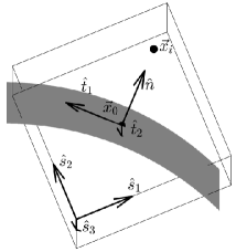
Figure 3: Patch used to define the correction function.

Here we use the “node-centered” [1] approach to construct the patches used to compute the correction function, as illustrated in figure 3 and described below.

Let us consider stencil $i\in S_{\Gamma}\/$, where $S_{\Gamma}\/$ is the set of stencils that straddle the interface. We denote $\ell_{i}\/$ as the maximum distance between grid points that are part of stencil $i$ (the characteristic length of the stencil), and $\vec{x}_{i}\/$ as the average position of those same grid points (the center position of the stencil). Furthermore, $P_{\Gamma}(\vec{x})\/$ denotes an approximate projection of $\vec{x}$ onto the interface $\Gamma\/$, defined as

$$P_{\Gamma}(\vec{x})=\vec{x}-\phi(\vec{x})\Biggl{(}\dfrac{\vec{\nabla}\phi(\vec{x})}{||\vec{\nabla}\phi(\vec{x})||^{2}}\Biggr{)}\/,$$ (7)

where $\phi\/$ is the level set function used to represent the interface.

The correction function patch associated with stencil $i$, denoted as $\Omega_{\Gamma_{i}}\/$, is a cube of edge length $\ell_{i}$ centered at $\vec{x}_{0_{i}}=P_{\Gamma}(\vec{x}_{i})\/$. Furthermore, the patch is oriented such that one of its diagonal planes coincides with the plane tangent to the interface at $\vec{x}_{0_{i}}\/$. Let $\hat{n}=\vec{\nabla}\phi(\vec{x}_{0_{i}})/||\vec{\nabla}\phi(\vec{x}_{0_{i}})||\/$ denote the unit vector normal to the interface at $\vec{x}_{0_{i}}\/$, and $\hat{t}_{1}\/$ and $\hat{t}_{2}\/$ denote vectors tangent to the surface, given by

$$\hat{t}_{1}=\hat{n}\times\hat{e}_{\min},\quad\hat{t}_{2}=\hat{n}\times\hat{t}_{1}\/,$$ (8)

where $\hat{e}_{\min}\/$ corresponds to the coordinate axis for which $(\hat{n}\cdot\hat{e}_{\min})\/$ is minimum. Then, define the following triad of unit vectors,

$$\hat{s}_{1}=(\hat{n}-\hat{t}_{1})/\sqrt{2}\/,\quad\hat{s}_{2}=(\hat{t}_{2}-\hat{s}_{1})\/,\quad\hat{s}_{3}=\hat{t}_{2}\/.$$

Finally, $\Omega_{\Gamma_{i}}\/$ is given by

$$\Omega_{\Gamma_{i}}=\left\{\vec{x}\;\bigg{|}\;\vec{x}=\vec{x}_{0_{i}}+\dfrac{\ell_{i}}{2}\sum_{i=1}^{3}\gamma_{i}\hat{s}_{i},\,\gamma_{i}\in[-1,1]\right\}.$$

2.3 Accuracy and robustness

The accuracy of the CFM stems from the fact that the correction function is defined as the solution to a PDE, which, in principle, can be solved to arbitrary order of accuracy. In the method described above, the accuracy is determined by the choice of basis functions used to represent $D\/$ within each patch. In this paper, as in ref. [1], we obtain fourth order of accuracy by representing $D\/$ with Hermite cubic interpolants.

In addition, the PDE that defines the correction function, and the least squares procedure used to solve it, do not depend on the computational grid. Hence, the CFM is applied exactly the same way for every discretization stencil that crosses the interface, and no special cases need to be considered. This feature makes the CFM very robust with respect to the arbitrary fashion an interface can cross the computational grid.

3 New technique for imposing jump conditions in a least squares sense

In this section we introduce a new technique for imposing the jump conditions in a least squares sense. This technique is based on two main observations:

1. The jump conditions can be enforced over any collection of surfaces that lie within a reasonable distance from the center of the correction function patch, and whose union has approximately the same area as a diagonal plane of the cubic patch.

2. The level set function can be used to define local coordinate transformations that map $L^{\infty}$ balls on the interface onto squares.

Hence, we impose the jump conditions on a collection of $L^{\infty}$ balls that satisfies observation (i) and, per observation (ii), over which we can easily integrate after appropriate coordinate transformations. These coordinate transformations are introduced in §3.1. In order to evaluate surface integrals, we also must be able to invert the (nonlinear) coordinate transformations efficiently. In §3.2 we present an algorithm to compute an approximate inverse of these transformations that only involves solving linear systems of equations. In §3.3 we show how to use the coordinate transformations, and their inverses, to impose jump conditions in a least squares sense. Finally, in §3.4 we discuss implementation details.

3.1 Local coordinate transformation

Let $\vec{x}_{q}$ denote a point on the interface $\Gamma\/$. Then, the following transformation maps a $L^{\infty}$ ball on the interface centered on $\vec{x}_{q}$ onto a square. This transformation is depicted in figure 4(a).

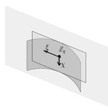
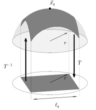
Figure 4: Local coordinate transformation $T_{q}\/$. Left: coordinates $\xi\/$ and $\chi\/$ are defined by the orthogonal projection onto the plane tangent to the interface at $\vec{x}_{q}\/$. Right: spherical interface of radius $r\/$. The transformation is bijective if $\ell_{q}<\sqrt{2}r\/$. The dark shaded region denotes $\mathcal{S}(\vec{x}_{q},\ell_{q})$.

Definition 1.

Local coordinate transformation. Let $\hat{n}\/$ denote the unit vector normal to the interface at $\vec{x}_{q}$, $\hat{t}_{1}\/$ and $\hat{t}_{2}\/$ denote vectors tangent to the surface, given by (8), and $\phi\/$ denote the level set function that represents $\Gamma\/$. Then, the local coordinate transformation $\{\eta,\xi,\chi\}=T_{q}(\vec{x})\/$ is given by

$$\eta=\dfrac{\phi}{||\vec{\nabla}\phi(\vec{x}_{q})||}\/,\quad\xi=\hat{t}_{1}\cdot(\vec{x}-\vec{x}_{q})\/,\quad\chi=\hat{t}_{2}\cdot(\vec{x}-\vec{x}_{q})\/.$$

In particular, consider the ball

$$\mathcal{S}(\vec{x}_{q},\ell_{q})=\{\vec{x}\in\Gamma\mid||\vec{x}-\vec{x}_{q}||_{n_{\infty}}\leq\ell_{q}\}\/,$$

where $||(.)||_{n_{\infty}}=\max(|(.)\cdot\hat{n}|,\,|(.)\cdot\hat{t}_{1}|,\,|(.)\cdot\hat{t}_{2}|)\/$. The transformation $T_{q}\/$ maps $\mathcal{S}(\vec{x}_{q},\ell_{q})$ onto the square $\{\xi,\chi\}\in[-\ell_{q}/2,\,\ell_{q}/2]^{2}\/$ on the $\eta=0\/$ plane.

If $\mathcal{S}(\vec{x}_{q},\ell_{q})$ is close enough to a plane (i.e., $\ell_{q}\/$ is much smaller than the minimum radius of curvature), the transformation is smooth and invertible in $\mathcal{S}(\vec{x}_{q},\ell_{q})$. To illustrate this fact, consider the simple case of a spherical interface of radius $r\/$, as depicted in figure 4(b). As long as $\mathcal{S}(\vec{x}_{q},\ell_{q})$ fits strictly within a half-sphere, the projection is smooth and invertible (because it is for any spherical cap smaller than a half-sphere). Simple geometry then shows that, in this case, the criterion for smoothness and invertibility is $\ell_{q}<\sqrt{2}r\/$. For an ellipsoid a similar argument shows that the criterion is $\ell_{q}<\sqrt{2}r_{\min}\/$ (note that any surface can be, locally, approximated by an ellipsoid). As discussed in §3.2, the algorithm used to approximate the inverse transformation $T_{q}^{-1}\/$ imposes a more stringent restriction to $\ell_{q}\/$.

In practice, we link $\ell_{q}\/$ to the size of the computational grid used to represent the level set function, and thus is set by the user. As described in §3.4, our implementation uses a convenient heuristics to check if the grid provided by the user has adequate refinement to satisfy the restrictions on $\ell_{q}\/$.

In addition, $\vec{x}_{q}$ need not lie exactly on the interface. If $\vec{x}_{q}$ is close to the interface (in the $\ell_{q}\/$-scale), then $\xi\/$ and $\chi\/$ are given by an orthogonal projection onto a plane approximately tangent to the interface. Hence $T_{q}\/$ is well defined, and the arguments above about smoothness and invertibility still apply.

3.2 Inverse transformation

Here we introduce an algorithm that computes an approximation to the inverse transformation $T_{q}^{-1}\/$. This algorithm avoids having to solve a nonlinear system of equations whenever an evaluation of $T_{q}^{-1}\/$ is required, which leads to significant computational savings.

Assume that the level set function $\phi\/$ is represented by a polynomial of degree $p\/$. Let $\hat{n}\/$ denote the unit vector normal to interface at $\vec{x}_{q}$, and $\hat{t}_{1}\/$ and $\hat{t}_{2}\/$ denote vectors that complete an orthonormal basis computed with (8). Then, we define $\mathcal{C}(\vec{x}_{q},\ell_{q})$ as a cube of edge length $\ell_{q}\/$ centered at $\vec{x}_{q}$, as follows,

$$\mathcal{C}(\vec{x}_{q},\ell_{q})=\left\{\vec{x}\;\bigg{|}\;\vec{x}=\vec{x}_{q}+\dfrac{\ell_{q}}{2}(\gamma_{1}\hat{t}_{1}+\gamma_{2}\hat{t}_{2}+\gamma_{3}\hat{n}),\,\gamma_{i}\in[-1,1]\right\}.$$

Figure 5 depicts the cube $\mathcal{C}(\vec{x}_{q},\ell_{q})$. Algorithm 1 computes an approximation to $T_{q}^{-1}\/$ within the region $T_{q}(\mathcal{C}(\vec{x}_{q},\ell_{q}))\/$ using a Hermite polynomial of degree $p\/$.

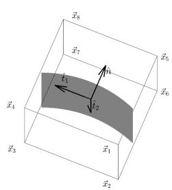
Figure 5: Cube $\mathcal{C}(\vec{x}_{q},\ell_{q})$ used to compute an approximation to the inverse transformation $T_{q}^{-1}\/$.

Algorithm 1 Approximate inverse transformation

1:Compute $\theta_{i}=T_{q}(\vec{x}_{i})\/$, where $\vec{x}_{i}\/$, $i=1,\ldots,8\/$ denotes the 8 vertices of $\mathcal{C}(\vec{x}_{q},\ell_{q})$.

2:Compute all derivatives $\partial^{|\alpha|}T_{q}(\vec{x}_{i})/\partial x^{\alpha_{1}}\partial y^{\alpha_{2}}\partial z^{\alpha_{3}}\/$, with $|\alpha|=\sum\alpha_{i}$, and $\max(\alpha_{i})\leq p-2\/$.

3:Using the inverse function theorem, compute all derivatives $\partial^{|\alpha|}T_{q}^{-1}(\theta_{i})/\partial\eta^{\alpha_{1}}\partial\xi^{\alpha_{2}}\partial\chi^{\alpha_{3}}\/$, with $\max(\alpha_{i})\leq p-2\/$.

4:Solve for the Hermite polynomial of degree $p\/$ that fits the inverse transformation at $\theta_{i}\/$.

The accuracy of the approximation to $T^{-1}\/$ imposes an upper bound on $\ell_{q}\/$. The Hermite interpolation results in an error $O(\ell_{q}^{p+1}D^{(p+1)}T^{-1})\/$, where $D^{(p+1)}\/$ denotes derivatives of order $p+1\/$. Hence, an accurate approximation is only possible when derivatives of order $p+1\/$ are bounded. Furthermore, the derivatives of $T^{-1}\/$ are related to the ratio $\ell_{q}/r_{\min}\/$, i.e., to how flat the section of the interface is with respect to $\ell_{q}\/$. We conjecture that, for a given $p\/$, it is possible to choose a constant $c>0\/$ such that $\ell_{q}<c\,r_{\min}\/$ guarantees $D^{(p+1)}T^{-1}=O(1)\/$. In particular, in our implementation we use $p=3\/$. For a spherical cap section of the interface, and $p=3\/$, one can show that $c\approx 0.4\/$. This observation motivates the heuristics we use to determine an upper bound for $\ell_{q}\/$, as discussed in §3.4.

3.3 Imposing jump conditions

Our goal is to impose jump conditions over a piece of the interface that includes enough information to define a unique solution to the Caucy problem (4) within each patch $\Omega_{\Gamma_{i}}\/$. In ref. [1] we show that in practice the method works well if these conditions are imposed over a piece of the interface whose area approximates the area of a diagonal plane of the correction function patch, and that is located within a ball of radius $O(\ell_{i})$ centered at the patch. There are many choices of surfaces that satisfy this heuristics. Previous implementations of the CFM impose jump conditions on the intersection between the interface and the correction function patch. Here we use the local transformation in §3.1 to define the section of interface over which the jump conditions are imposed, which simplifies the computation of surface integrals via numerical quadrature.

Given $\vec{x}_{q}\in\Gamma\/$, the corresponding local transformation $T_{q}\/$, and its inverse $T_{q}^{-1}\/$, one can evaluate the square error in satisfying the jump conditions over the surface $\mathcal{S}(\vec{x}_{q},\ell_{q})$ as follows:

$$\begin{split}\int_{\mathcal{S}(\vec{x}_{q},\ell_{q})}\mathscr{E}\,dS&=\int_{-\ell_{s}/2}^{\ell_{s}/2}\int_{-\ell_{s}/2}^{\ell_{s}/2}\mathscr{E}(T_{q}^{-1}\bigl{(}0,\xi,\chi)\bigr{)}\biggl{\lVert}\dfrac{\partial\vec{x}}{\partial\xi}\times\dfrac{\partial\vec{x}}{\partial\chi}\biggr{\rVert}\,d\xi\,d\chi\/\\[5.0pt] &\approx\sum_{j}\Biggl{(}w_{j}\,\mathscr{E}(T_{q}^{-1}\bigl{(}0,\xi_{j},\chi_{j})\bigr{)}\biggl{\lVert}\dfrac{\partial\vec{x}}{\partial\xi}\times\dfrac{\partial\vec{x}}{\partial\chi}\biggr{\rVert}_{(0,\xi_{j},\chi_{j})}\Biggr{)}\/,\end{split}$$ (9)

where

$$\mathscr{E}=(D-a)^{2}+\ell_{i}^{2}(D_{n}-b)^{2}\/,$$

$w_{j}\/$ are the weights of a numerical quadrature defined over the square $[-\ell_{q}/2,\ell_{q}/2]^{2}\/$, and $(\xi_{j},\chi_{j})\/$ are the quadrature points.

As discussed in §3.4, the location of the points $\vec{x}_{q}\/$ and the length $\ell_{q}\/$ are defined by the computational grid used to represent the level set function. In general, the patch $\Omega_{\Gamma_{i}}\/$ can intersect several sections $\mathcal{S}(\vec{x}_{q},\ell_{q})$, each associated with a different $\vec{x}_{q}$, as illustrated by figure 6. Hence, within each patch we impose the jump conditions over the union of all $\mathcal{S}(\vec{x}_{q},\ell_{q})$ regions associated with the set $Q=\{q\mid||\vec{x}_{q}-\vec{x}_{0_{i}}||_{2}<\sqrt{2}/2\,\ell_{i}\/\}\/$. We incorporate this new technique of imposing jump conditions into the CFM by modifying the minimization functional (6) to

$$\begin{split}J_{i}^{\text{new}}&=\dfrac{\ell_{i}^{4}}{V_{i}}\int_{\Omega_{\Gamma_{i}}}(\nabla^{2}D-f_{D})^{2}dV\\ &+\dfrac{1}{\tilde{S}_{i}}\sum_{q\in Q}\int_{\mathcal{S}(\vec{x}_{q},\ell_{q})}[(D-a)^{2}+\ell_{i}^{2}(D_{n}-b)^{2}]dS\/,\end{split}$$ (10)

where $\tilde{S}_{i}=\sum_{q\in Q}S_{q}\/$, and $S_{q}\/$ denotes the area of $\mathcal{S}(\vec{x}_{q},\ell_{q})$.

3.4 Implementation details

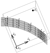
Figure 6: The surface integrals are evaluated over $L^{\infty}$ balls over the interface. The sections may overlap, and one patch may contain several sections.

We use the discretization of the level set function $\phi\/$ to compute the set of points $\vec{x}_{q}\/$ and to determine the length $\ell_{q}\/$. Let $G_{\Gamma}\/$ denote the grid used to discretize $\phi\/$, and $\mathcal{X}_{\Gamma}\/$ denote the set of grid cells in $G_{\Gamma}\/$ that are crossed by the interface. Then, for each cell $q\in\mathcal{X}_{\Gamma}$ we set $\ell_{q}\/$ as the diagonal length of the cell, and $\vec{x}_{q}=P_{\Gamma}(\vec{x}_{c_{q}})\/$, where $\vec{x}_{c_{q}}\/$ denotes the center of the cell. This implementation assumes that $G_{\Gamma}\/$ is fine enough to “resolve” the interface $\Gamma\/$, such that the local transformation $T_{q}\/$ is smooth and invertible, and that the approximate algorithm used to compute $T_{q}^{-1}\/$ is accurate.

In practice, we assess the adequateness of $\ell_{q}\/$ by monitoring the determinant of the Jacobian on the $\xi-\chi\/$ plane,

$$\text{Jac}=\biggl{\lVert}\dfrac{\partial\vec{x}}{\partial\xi}\times\dfrac{\partial\vec{x}}{\partial\chi}\biggr{\rVert}_{T^{-1}(0,\xi,\chi)}\/,$$ (11)

evaluated at the quadrature points used to compute the surface integral (9). Since (11) is computed to impose the jump conditions, computing this indicator does not add to the computational cost. For a spherical cap section of the interface we can show that $\ell_{q}<0.4\,r\/$ implies $\text{Jac}>0.83\/$ (see §3.2 for the motivation for this limitation on $\ell_{q}\/$). Hence, we use this threshold to verify whether $\ell_{q}\/$ is small enough in general cases.

Furthermore, to guarantee that $G_{\Gamma}\/$ can always be made as fine as needed, we allow $G_{\Gamma}\/$ to be distinct from the grid used to solve the Poisson equation. We make this distinction explicit by denoting the grid in which the Poisson equation is solved by $G_{P}\/$.

4 Results

In this section we verify the accuracy and robustness of the proposed technique for imposing jump conditions with numerical examples in 2-D and 3-D.

The results shown here are computed with an overall fourth order accurate scheme. Namely, we discretize Poisson’s equation using the standard 9-point stencil in 2-D, and the equivalent 19-point stencil in 3-D. Furthermore, we represent the correction function with Hermite cubic polynomials, which is consistent with fourth order of accuracy. Finally, we represent the interfaces using the Gradient-Augmented Level-Set (GALS) method [41], which is also based on Hermite cubic polynomials.

Below we use analytic expressions to define the model problems, but only the appropriate discrete data defined on a computational grid are used as inputs to the code (this is close to a practical situation in which data defining the interface is the result of a computation on the same grid). The data is presented in terms of the exact solution (denoted by $u\/$), and the level set function (denoted by $\phi\/$). We verify accuracy by evaluating the $L^{\infty}\/$ norm of the error in the solution and its gradient. Furthermore, in some problems the resolutions of $G_{P}\/$ (grid where Poisson’s equation is solved) and $G_{\Gamma\/}$ (grid where the level set function is defined) are distinct. In these cases we maintain the resolution ratio between these grids constant during error convergence studies.

In the first two examples we compare the accuracy of the technique presented here to the approach used in ref. [1] to solve 2-D problems. The CFM implemented in ref. [1] differs from the current work in three main aspects: (i) the patch used to compute the correction function, (ii) the weight given to the jump condition in the least squares minimization (5–6), and (iii) the technique used to compute the integrals along the interface. Since the focus of the present paper is point (iii), in these examples we compute two sets of solutions: minimizing (10) with the integration technique of §3 (coordinate transformation), and minimizing (6) with the integration technique of ref. [1] (curve parametrization). Both solutions are based on the patch construction described in §2.2. We compare these solutions with the results presented in ref. [1].

4.1 Smooth 5-pointed star

Here we reproduce example 2 of ref. [1], which involves a smooth 5-pointed star. By considering a smooth interface we guarantee that the transformation introduced in §3.1 is well defined, without the need of special considerations near singular points (e.g., corners). In this example $G_{P}$ and $G_{\Gamma}$ are the same grid. The problem is defined as follows.

• $\phi(x\/,\,y)=(x-0.5)^{2}+(y-0.5)^{2}-\big{(}0.25+0.05\sin(5\varphi(x\/,\,y)\big{)}^{2}\/$.

• $\varphi(x\/,\,y)=\arctan\Big{(}\dfrac{y-0.5}{x-0.5}\Big{)}\/$.

• $\Omega_{1}=\{(x\/,\,y)\in[0,1]^{2}\mid\phi(x\/,\,y)\leq 0\}\/$.

• $\Omega_{2}=\{(x\/,\,y)\in[0,1]^{2}\mid\phi(x\/,\,y)>0\}\/$.

• $u_{1}(x\/,\,y)=\exp(x)\cos(y)\/$.

• $u_{2}(x\/,\,y)=0\/$.

Figure 7 shows the interface immersed into the Cartesian grid $G_{P}$ used to solve the Poisson equation, along with a plot of the solution obtained with the CFM. Figure 8 shows the error obtained with the present technique (coordinate transformation), the current version of the CFM with integration technique of ref. [1] (curve parametrization), and the results presented in ref. [1]. All three versions of the CFM present fourth order of accuracy and comparable errors.

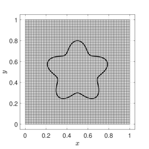
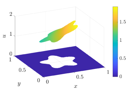
Figure 7: Example 1. Left: interface immersed into $G_{P}\/$. Right: Solution given by the CFM.

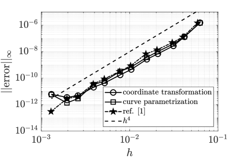
Figure 8: Example 1. Error convergence in the $L^{\infty}\/$ norm. Comparison of results computed by evaluating surface integrals with coordinate transformation (current work), curve parametrization, and results presented in ref. [1].

4.2 Touching circles

Here we reproduce example 5 of ref. [1], which involves two circular interfaces that touch at one point. In this example the interfaces are represented by level set functions defined on independent grids: $G_{\Gamma_{1}}\/$ and $G_{\Gamma_{2}}\/$. To be consistent with the implementation of ref. [1], we choose $G_{\Gamma_{1}}\/$ and $G_{\Gamma_{2}}\/$ to be the same as $G_{P}\/$. The problem is defined as follows.

• $\phi_{1}(x\/,\,y)=\big{(}x-0.5-0.2\cos(\pi/e^{2})\big{)}^{2}+\big{(}y-0.5-0.2\sin(\pi/e^{2})\big{)}^{2}-0.01\/$.

• $\phi_{2}(x\/,\,y)=(x-0.5)^{2}+(y-0.5)^{2}-0.09\/$.

• $\Omega_{1}=\{(x\/,\,y)\in[0,1]^{2}\mid\phi_{1}(x\/,\,y)\leq 0\}$.

• $\Omega_{2}=\{(x\/,\,y)\in[0,1]^{2}\mid\phi_{1}(x\/,\,y)>0,\phi_{2}(x\/,\,y)\leq 0\}\/$.

• $\Omega_{3}=\{(x\/,\,y)\in[0,1]^{2}\mid\phi_{1}(x\/,\,y)>0,\phi_{2}(x\/,\,y)>0\}\/$.

• $u_{1}(x\/,\,y)=\sin(\pi x)\sin(\pi y)+5\/$.

• $u_{2}(x\/,\,y)=\sin(\pi x)\big{(}\sin(\pi y)-\exp(\pi y)\big{)}\/$.

• $u_{3}(x\/,\,y)=\exp(x)\big{(}x^{2}\sin(y)+y^{2}\big{)}\/$.

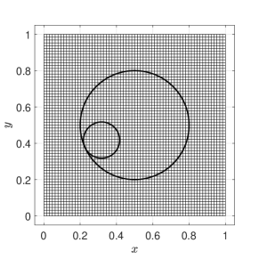
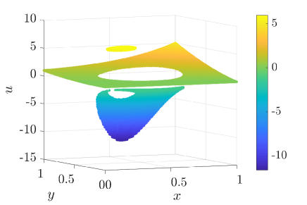
Figure 9: Example 2. Left: interfaces immersed into $G_{P}\/$, with circles that touch at single point. Right: solution obtained with the CFM.

Figure 9 shows the interfaces immersed into the Cartesian grid $G_{P}$ used to solve the Poisson equation, along with a plot of the solution obtained with the CFM. Since the jump conditions (1b-c) are linear, one can solve for correction functions associated with each interface independently and combine them as needed – see remark 4. As shown in fig. 9, this approach allows for arbitrarily close interfaces

Remark 4.

In practice, the interfaces seen by the CFM are subject to errors due to the level set representation. Hence, the “effective” interfaces likely do not touch perfectly at just one point. They may cross over, or not touch at all. However, the CFM can handle these situations seamlessly by computing correction functions due to each of the interfaces independently. For instance, when the solution domain is subdivided into three regions by two interfaces, such as in figure 9, the CFM computes $D_{12}=u_{2}-u_{1}\/$ and ${D_{13}=u_{3}-u_{1}}\/$, where $u_{i}\/$ denotes the solution restricted to each of the three regions. Since the jump conditions (1b-c) are linear, these correction functions can be combined to compute ${D_{23}=u_{3}-u_{2}=D_{13}-D_{12}}\/$ as needed.   $\clubsuit\/$

Figure 10 shows the error obtained with the present technique (coordinate transformation), the current version of the CFM with integration technique of ref. [1] (curve parametrization), and the results presented in ref. [1]. Once again, all three versions of the CFM present fourth order of accuracy and comparable errors.

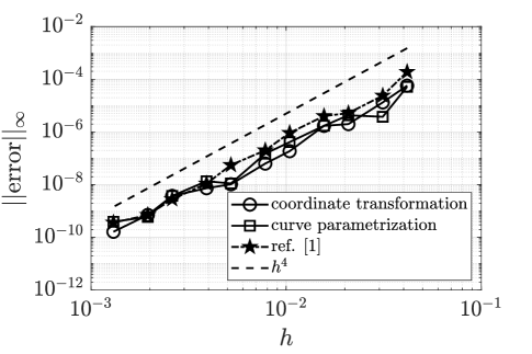
Figure 10: Example 2. Error convergence in the $L^{\infty}\/$ norm. Comparison of results computed by evaluating surface integrals with coordinate transformation (current work), curve parametrization, and results presented in ref. [1].

4.3 Three interfaces in 2-D

This 2-D example, which is not in [1], illustrates the application of the new implementation of the CFM to solve problems with more than two interfaces close together. We solve the following problem with three interfaces:

• $\phi_{1}(x_{1}\/,\,y_{1})=(x_{1}-0.3)^{2}+(y_{1}-0.3)^{2}-0.05\/$.

• $\phi_{2}(x_{2}\/,\,y_{2})=(x_{2}-0.3)^{2}+(y_{2}-0.3)^{2}-\bigl{(}\sqrt{3}/10+0.05\sin(5\varphi_{2}(x_{2}\/,\,y_{2})\bigr{)}^{2}\/$.

• $\phi_{2}(x_{3}\/,\,y_{3})=(x_{3}-0.25)^{2}+(y_{3}-0.25)^{2}-\big{(}0.15+0.05\sin(2\varphi_{3}(x_{3}\/,\,y_{3})\big{)}^{2}\/$.

• $\varphi_{2}(x_{2}\/,\,y_{2})=\arctan\Big{(}\dfrac{y_{2}-0.3}{x_{2}-0.3}\Big{)}\/$.

• $\varphi_{3}(x_{3}\/,\,y_{3})=\arctan\Big{(}\dfrac{y_{3}-0.25}{x_{3}-0.25}\Big{)}\/$.

• $\Omega_{1}=\{(x_{1}\/,\,y_{1})\in[0,0.6]^{2}\mid\phi_{1}(x_{1}\/,\,y_{1})\leq 0\}\/$.

• $\Omega_{2}=\{(x_{2}\/,\,y_{2})\in[0,0.6]^{2}\mid\phi_{2}(x_{2}\/,\,y_{2})\leq 0\}\/$.

• $\Omega_{3}=\{(x_{3}\/,\,y_{3})\in[0,0.5]^{2}\mid\phi_{3}(x_{3}\/,\,y_{3})\leq 0\}\/$.

• $\Omega_{4}=\{(x\/,\,y)\in[0,1]^{2}\,|\,\phi_{i}(x\/,\,y)>0,i=1\/,\,2\/,\,3\}\/$.

• $u_{1}(x\/,\,y)=\exp(x)\big{(}x^{2}\sin(y)+y^{2}\big{)}\/$.

• $u_{2}(x\/,\,y)=\sin(\pi x)\sin(\pi y)+10\/$.

• $u_{3}(x\/,\,y)=x\,y+10\/$.

• $u_{4}(x\/,\,y)=10(x^{2}+y^{2})\/$.

In this example the level set grids ($G_{\Gamma_{1}}\/$, $G_{\Gamma_{2}}\/$, and $G_{\Gamma_{3}}\/$) are not the same as $G_{P}\/$. The relationships between the grid spacings are $h_{\Gamma_{1}}/h_{P}=h_{\Gamma_{2}}/h_{P}=0.6$ and $h_{\Gamma_{3}}/h_{P}=0.5$. In the expressions above, each level set is defined in terms of the Cartesian coordinates aligned with the corresponding grid. These coordinates are defined as follows:

$$x_{1} =x-0.34,$$

$$y_{1} =y-0.37,$$

$$x_{2} =(x-0.29)\cos(35\pi/180)+(y+0.1)\sin(35\pi/180)\/,$$

$$y_{2} =-(x-0.29)\sin(35\pi/180)+(y+0.1)\cos(35\pi/180)\/,$$

$$x_{3} =(x-0.885)\cos(75\pi/180)+(y+0.048)\sin(75\pi/180)\/,$$

$$y_{3} =-(x-0.885)\sin(75\pi/180)+(y+0.048)\cos(75\pi/180)\/.$$

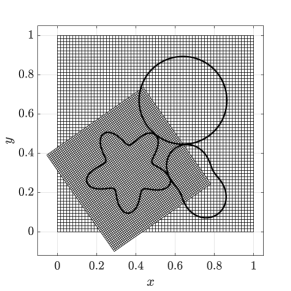
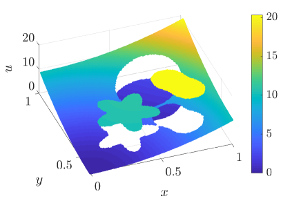
Figure 11: Example 3. Left: interfaces immersed into $G_{P}\/$. The grid $G_{\Gamma_{2}}\/$ used to represent $\phi_{2}\/$ is also shown. Right: solution obtained with the CFM.

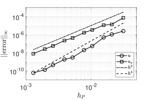
Figure 12: Example 3. Convergence of the error of in the solution and its $x$-derivative in the $L^{\infty}\/$ norm. The $y$-derivative behaves similarly.

We illustrate the concept of independent level set grids in figure 11(left). In this figure we show $G_{\Gamma_{2}}\/$ laid over $G_{P}\/$, along with the immersed interfaces. The solution obtained with the CFM is shown in figure 11(right). Once again we observe that the CFM produces good results in the presence of multiple interfaces. Furthermore, in addition to the expected fourth order convergence of the error in the solution, we also observe third order convergence of the error in the gradient, as shown in figure 12.

4.4 Sphere with bumps

In this example we solve the following 3-D problem, which is illustrated in figure 13.

• $\phi(x_{1}\/,\,y_{1}\/,\,z_{1})=(x_{1}-0.35)^{2}+(y_{1}-0.35)^{2}+(z_{1}-0.35)^{2}-r^{2}\/$.

• $r(\varphi\/,\,\psi)=\sqrt{3}/8+(0.28/\pi)(\varphi-\varphi^{2}/\pi)\sin(3\varphi)\sin(4\psi)\/$.

• $\varphi(x_{1}\/,\,y_{1})=\arctan\Big{(}\dfrac{y_{1}-0.35}{x_{1}-0.35}\Big{)}\/$.

• $\psi(x_{1}\/,\,y_{1}\/,\,z_{1})=\arccos\Bigg{(}\dfrac{z_{1}-0.35}{\sqrt{(x_{1}-0.35)^{2}+(y_{1}-0.35)^{2}+(z_{1}-0.35)^{2}}}\Bigg{)}\/$.

• $\Omega_{1}=\{(x_{1}\/,\,y_{1}\/,\,z_{1})\in[0,0.7]^{3}\mid\phi(x_{1}\/,\,y_{1}\/,\,z_{1})\leq 0\}\/$.

• $\Omega_{2}=\{(x\/,\,y\/,\,z)\in[0,1]^{3}\mid\phi(x\/,\,y\/,\,z)>0\}\/$.

• $u_{1}(x\/,\,y\/,\,z)=\sin(\pi(x+z)/\sqrt{2})\exp(\pi y)\/$.

• $u_{2}(x\/,\,y\/,\,z)=0\/$.

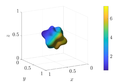
Figure 13: Example 4. Interface immersed into $G_{P}\/$, colored according to the intensity of the jump in the solution across it.

In the expressions above, the level set $\phi\/$ is defined in terms of the Cartesian coordinates aligned with $G_{\Gamma}\/$. These coordinates are given by

$$x_{1} =x-0.13\/,$$

$$y_{1} =y-0.1\/,$$

$$z_{1} =z-0.15\/.$$

Note that $G_{\Gamma}\/$ is distinct from $G_{P}\/$, and the relationship between grid spacings is $h_{\Gamma}/h_{P}=0.7$.

Figure 13 shows the interface, colored according to the intensity in the jump in the solution across it. Figure 14 shows a 2-D slice of the 3-D solution computed with the CFM, as well as the interface immersed into the Cartesian grid at the slicing plane. The error of the solution and its gradient are plotted in figure 15. Just as in 2-D, the accuracy is fourth order in the solution and third order in the gradient.

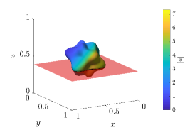
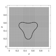
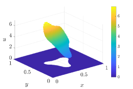
Figure 14: Example 4. 2-D slice of the 3-D solution. Left: location of the slicing plane ($z=0.39$). Center: grid $G_{P}\/$. Right: solution obtained with the CFM.

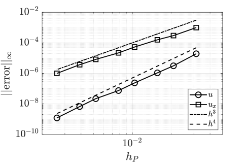
Figure 15: Example 4. Convergence of the error in the solution and its $x$-derivative in the $L^{\infty}\/$ norm. The $y\/$ and $z$-derivatives behave similarly.

4.5 Touching spheres

Here we present a 3-D version of example 2 in §4.2. We consider two spherical interfaces that touch at a single point, as shown in figure 16. The interfaces are each represented using independent level set grids and the relationships between grid spacings are $h_{\Gamma_{1}}/h_{P}=0.8$ and $h_{\Gamma_{2}}/h_{P}=0.5$. The problem is defined as follows:

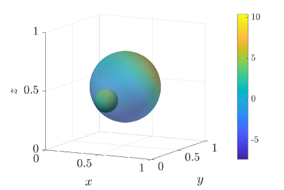
Figure 16: Example 5. Interfaces immersed into $G_{P}\/$, colored according to the intensity of the jumps in the solution across them. The spheres touch at a single point. Transparency is applied to the outer interface to show the internal interface.

• $\phi_{1}(x_{1}\/,\,y_{1}\/,\,z_{1})=(x_{1}-0.40)^{2}+(y_{1}-0.40)^{2}+(z_{1}-0.40)^{2}-0.09\/$.

• $\phi_{2}(x_{2}\/,\,y_{2}\/,\,z_{2})=(x_{2}-0.25)^{2}+(y_{2}-0.25)^{2}+(z_{2}-0.25)^{2}-0.01\/$.

• $\Omega_{1}=\{(x_{1}\/,\,y_{1}\/,\,z_{1})\in[0,0.8]^{3}\mid,\phi_{1}(x_{1}\/,\,y_{1}\/,\,z_{1})\leq 0\}\/$.

• $\Omega_{2}=\{(x_{2}\/,\,y_{2}\/,\,z_{2})\in[0,0.5]^{3}\mid\phi_{2}(x_{2}\/,\,y_{2}\/,\,z_{2})\leq 0\}\/$.

• $\Omega_{3}=\{(x\/,\,y\/,\,z)\in[0,1]^{3}\mid\phi_{1}(x\/,\,y\/,\,z)>0,\phi_{2}(x\/,\,y\/,\,z)>0\}\/$.

• $u_{1}(x\/,\,y\/,\,z)=\bigl{(}\sin(\pi x)\sin(\pi y)+5\bigr{)}\log(x+z+2)\/$.

• $u_{2}(x\/,\,y\/,\,z)=\sin\bigl{(}\pi(x+z)\bigr{)}\bigl{(}\sin(\pi y)-\exp(\pi y)\bigr{)}\/$.

• $u_{3}(x\/,\,y\/,\,z)=\exp(x)\bigl{(}x^{2}\sin(y)+y^{2}\bigr{)}\cos(\pi z)\/$.

In the expressions above, the level sets are defined in terms of the respective grid coordinates, which are given by

$$x_{1} =x-0.1\/,$$

$$y_{1} =y-0.1\/,$$

$$z_{1} =z-0.1\/,$$

$$x_{2} =x-0.25-0.2\cos(\pi/e^{2})\cos(\pi/3\varphi)\/,$$

$$y_{2} =y-0.25-0.2\sin(\pi/e^{2})\cos(\pi/3\varphi)\/,$$

$$z_{2} =z-0.25-0.2\sin(\pi/3\varphi)\/,$$

where $\varphi\/$ denotes the golden ratio, $\varphi=\frac{1+\sqrt{5}}{2}\/$.

Figure 16 shows the interfaces, colored according to the intensity of the jumps in the solution across them. Figure 17 shows a 2-D slice of the 3-D solution, as computed with the CFM, on a plane close to the contact point between the spheres. The error in the solution and gradient are plotted in figure 18. Note that the accuracy of the solution and gradient does not degrade, even though the interfaces are arbitrarily close.

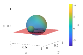
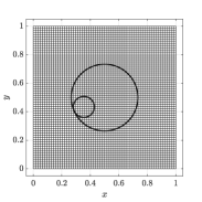
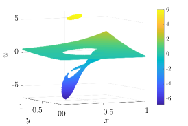
Figure 17: Example 5. 2-D slice of the 3-D solution. Left: location of the slicing plane ($z=0.32$). Center: grid $G_{P}\/$. Right: solution obtained with the CFM.

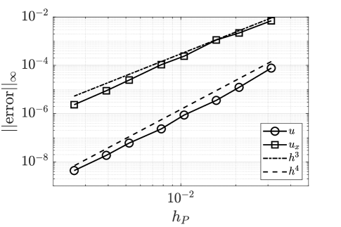
Figure 18: Example 5. Convergence of the error in the solution and its $x$-derivative in the $L^{\infty}\/$ norm. The $y\/$ and $z$-derivatives behave similarly.

4.6 3-D interfaces touching at two points

In this last example we apply the CFM to a 3-D problem with two interfaces that touch at two points, as shown in figure 19. The interfaces are represented using separate level set grids and the relationships between the grid spacings are $h_{\Gamma_{1}}/h_{P}=0.85$ and $h_{\Gamma_{2}}/h_{P}=0.6$. The problem is defined as follows:

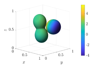
Figure 19: Example 6. Interfaces immersed into $G_{P}\/$, colored according to the intensity of the jumps in the solution across them. The interfaces touch at two distinct points.

• $R=\sqrt{(x_{1}-0.425)^{2}+(y_{1}-0.425)^{2}+(z_{1}-0.425)^{2}}\/$.

• $\psi(x_{1}\/,\,y_{1}\/,\,z_{1})=\arccos\Biggl{(}\dfrac{z_{1}-0.425}{R^{2}}\Biggr{)}\/$.

• $r(\psi)=0.25+0.13\cos(2\psi)\/$.

• $\phi_{1}(x_{1}\/,\,y_{1}\/,\,z_{1})=R^{2}-r^{2}\/$

• $\phi_{2}(x_{2}\/,\,y_{2}\/,\,z_{2})=(x_{2}-0.3)^{2}+(y_{2}-0.3)^{2}+(z_{2}-0.3)^{2}-0.04\/$.

• $\Omega_{1}=\{(x_{1}\/,\,y_{1}\/,\,z_{1})\in[0,0.85]^{3}\mid\phi_{1}(x_{1}\/,\,y_{1}\/,\,z_{1})\leq 0\}\/$.

• $\Omega_{2}=\{(x_{2}\/,\,y_{2}\/,\,z_{2})\in[0,0.6]^{3}\mid\phi_{2}(x_{2}\/,\,y_{2}\/,\,z_{2})\leq 0\}\/$.

• $\Omega_{3}=\{(x\/,\,y\/,\,z)\in[0,1]^{3}\mid\phi_{1}(x\/,\,y\/,\,z)>0,\phi_{2}(x\/,\,y\/,\,z)>0\}\/$.

• $u_{1}(x\/,\,y\/,\,z)=x\,y\,z\/$.

• $u_{2}(x\/,\,y\/,\,z)=\exp(x)\cos(y)\sin(z)\/$.

• $u_{3}(x\/,\,y\/,\,z)=\log\bigl{(}\sqrt{(x-0.661)^{2}+(y-0.651)^{2}+(z-0.636)^{2}}\bigr{)}\/$.

Note that, in the expressions above, the level set functions are defined in terms of their respective grid coordinates, given by

$$x_{1} =(x-0.1)\cos(10\pi/180)+(z-0.05)\sin(10\pi/180)\/,$$

$$y_{1} =y-0.05\/,$$

$$z_{1} =-(x-0.1)\sin(10\pi/180)+(z-0.05)\cos(10\pi/180)\/,$$

$$x_{2} =x-0.1047\/,$$

$$y_{2} =y-0.1842\/,$$

$$z_{2} =z-0.1249\/.$$

Figure 19 shows the interfaces, colored according to the intensity of the jump in the solution across them. Figure 20 shows a 2-D slice of the 3-D solution, as computed with the CFM, on a plane close to one of the contact points. The errors in the solution and its gradient are plotted in figure 21. These results corroborate the accuracy of this CFM implementation, as well as its robustness with respect to situations with arbitrarily close interfaces.

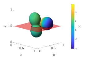
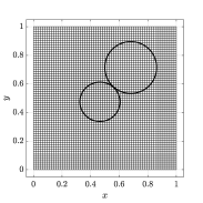
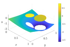
Figure 20: Example 6. 2-D slice of the 3-D solution. Left: location of the slicing plane ($z=0.5$). Center: grid $G_{P}\/$. Right: solution obtained with the CFM.

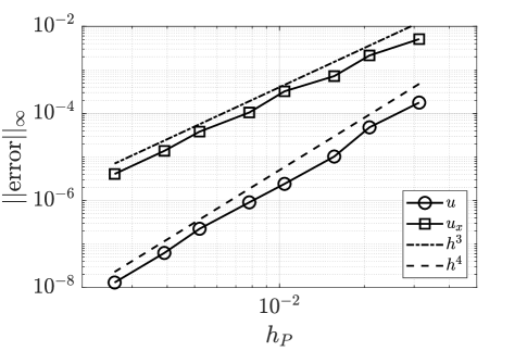
Figure 21: Example 6. Convergence of the error in the solution and its $x$-derivative in the $L^{\infty}\/$ norm. The other derivatives behave similarly.

5 Conclusion

We present a new technique to impose jump conditions in a least squares sense in the context of the Correction Function Method (CFM). This technique results in a re-formulation of the CFM that significantly simplifies numerical evaluation of surface integrals associated with the jump conditions, especially when only an implicit representation of the interface is available (e.g., the zero contour of a level set function). Furthermore, this new formulation preserves the main features of the CFM: high order of accuracy and compact discretization stencils.

The technique introduced here uses approximate coordinate transformations to map $L^{\infty}\/$ balls on the interface onto squares, defining interface sections over which integration can be carried out easily using standard numerical quadrature. The technique also exploits the flexibility of the CFM framework to create a least squares formulation that only involves integrals over collections of such $L^{\infty}\/$ balls, resulting in simple integral evaluations.

We show with numerical experiments that the reformulation of the CFM incorporating the new technique is efficient, accurate, and robust with respect to the arbitrary fashion in which the interface can intersect the computational grid. In particular, we show fourth order of accuracy when solving Poisson’s equation (1) when the diffusion coefficient $\beta\/$ is constant. An extension of this approach to problems involving discontinuous $\beta\/$ is the subject of current work.

References

References

- [1] A. N. Marques, J.-C. Nave, R. R. Rosales, A Correction Function Method for Poisson problems with interface jump conditions, Journal of Computational Physics 230 (20) (2011) 7567–7597. doi:10.1016/j.jcp.2011.06.014.
- [2] A. N. Marques, A Correction Function Method to solve incompressible fluid flows to high accuracy with immersed geometries, Ph.D. thesis, Massachusetts Institute of Technology (2012).
- [3] A. N. Marques, J.-C. Nave, R. R. Rosales, High order solution of Poisson problems with piecewise constant coefficients and interface jumps, Journal of Computational Physics 335 (2017) 497 – 515. doi:10.1016/j.jcp.2017.01.029.
- [4] X. Wen, High order numerical methods to three dimensional delta function integrals in level set methods, SIAM Journal on Scientific Computing 32 (3) (2010) 1288–1309. doi:10.1137/090758295.
- [5] B. Müller, F. Kummer, M. Oberlack, Highly accurate surface and volume integration on implicit domains by means of moment-sfitting, International Journal for Numerical Methods in Engineering 96 (8) (2013) 512–528. doi:10.1002/nme.4569.
- [6] R. Saye, High-order quadrature methods for implicitly defined surfaces and volumes in hyperrectangles, SIAM Journal on Scientific Computing 37 (2) (2015) A993–A1019. doi:10.1137/140966290.
- [7] P. Schwartz, J. Percelay, T. Ligocki, H. Johansen, D. Graves, D. Devendran, P. Colella, E. Ateljevich, High-accuracy embedded boundary grid generation using the divergence theorem, Communications in Applied Mathematics and Computational Science 10 (1) (2015) 83–96. doi:10.2140/camcos.2015.10.83.
- [8] T. Fries, S. Omerović, Higher-order accurate integration of implicit geometries, International Journal for Numerical Methods in Engineering 106 (5) (2016) 323–371. doi:10.1002/nme.5121.
- [9] C. S. Peskin, Flow patterns around heart valves: A numerical method, Journal of Computational Physics 10 (2) (1972) 252 – 271. doi:10.1016/0021-9991(72)90065-4.
- [10] C. S. Peskin, Numerical analysis of blood flow in the heart, Journal of Computational Physics 25 (3) (1977) 220–252. doi:10.1016/0021-9991(77)90100-0.
- [11] C. S. Peskin, B. F. Printz, Improved volume conservation in the computation of flows with immersed elastic boundaries, Journal of Computational Physics 105 (1) (1993) 33 – 46. doi:10.1006/jcph.1993.1051.
- [12] D. Goldstein, R. Handler, L. Sirovich, Modeling a no-slip flow boundary with an external force field, Journal of Computational Physics 105 (2) (1993) 354 – 366. doi:10.1006/jcph.1993.1081.
- [13] M.-C. Lai, C. S. Peskin, An immersed boundary method with formal second-order accuracy and reduced numerical viscosity, Journal of Computational Physics 160 (2) (2000) 705–719. doi:10.1006/jcph.2000.6483.
- [14] R. Cortez, M. Minion, The Blob Projection Method for immersed boundary problems, Journal of Computational Physics 161 (2) (2000) 428 – 453. doi:10.1006/jcph.2000.6502.
- [15] C. S. Peskin, The immersed boundary method, Acta Numerica 11 (2002) 479–517. doi:10.1017/S0962492902000077.
- [16] B. E. Griffith, C. S. Peskin, On the order of accuracy of the immersed boundary method: Higher order convergence rates for sufficiently smooth problems, Journal of Computational Physics 208 (1) (2005) 75–105. doi:10.1016/j.jcp.2005.02.011.
- [17] R. Mittal, G. Iaccarino, Immersed boundary methods, Annual Review of Fluid Mechanics 37 (1) (2005) 239–261. doi:10.1146/annurev.fluid.37.061903.175743.
- [18] D. B. Stein, R. D. Guy, B. Thomases, Immersed boundary smooth extension: A high-order method for solving PDE on arbitrary smooth domains using fourier spectral methods, Journal of Computational Physics 304 (2016) 252–274. doi:10.1016/j.jcp.2015.10.023.
- [19] H. Johansen, P. Colella, A Cartesian grid embedded boundary method for Poisson’s equation on irregular domains, Journal of Computational Physics 147 (1) (1998) 60–85. doi:10.1006/jcph.1998.5965.
- [20] A. Mayo, The fast solution of Poisson’s and the biharmonic equations on irregular regions, SIAM Journal on Numerical Analysis 21 (2) (1984) 285–299. doi:10.1137/0721021.
- [21] A. Mayo, The rapid evaluation of volume integrals of potential theory on general regions, Journal of Computational Physics 100 (2) (1992) 236–245. doi:10.1016/0021-9991(92)90231-M.
- [22] A. McKenney, L. Greengard, A. Mayo, A fast Poisson solver for complex geometries, Journal of Computational Physics 118 (2) (1995) 348 – 355. doi:10.1006/jcph.1995.1104.
- [23] R. J. LeVeque, Z. Li, The Immersed Interface Method for elliptic equations with discontinuous coefficients and singular sources, SIAM Journal on Numerical Analysis 31 (4) (1994) 1019–1044. doi:10.1137/0731054.
- [24] R. J. LeVeque, Z. Li, Immersed Interface Methods for Stokes flow with elastic boundaries or surface tension, SIAM Journal on Scientific Computing 18 (3) (1997) 709–735. doi:10.1137/S1064827595282532.
- [25] Z. Li, M.-C. Lai, The Immersed Interface Method for the Navier-Stokes equations with singular forces, Journal of Computational Physics 171 (2) (2001) 822–842. doi:10.1006/jcph.2001.6813.
- [26] L. Lee, R. J. LeVeque, An Immersed Interface Method for incompressible Navier-Stokes equations, SIAM Journal on Scientific Computing 25 (3) (2003) 832–856. doi:10.1137/S1064827502414060.
- [27] M. N. Linnick, H. F. Fasel, A high-order immersed interface method for simulating unsteady incompressible flows on irregular domains, Journal of Computational Physics 204 (1) (2005) 157 – 192. doi:10.1016/j.jcp.2004.09.017.
- [28] X. Zhong, A new high-order immersed interface method for solving elliptic equations with imbedded interface of discontinuity, Journal of Computational Physics 225 (1) (2007) 1066 – 1099. doi:10.1016/j.jcp.2007.01.017.
- [29] R. P. Fedkiw, T. Aslam, B. Merriman, S. Osher, A non-oscillatory Eulerian approach to interfaces in multimaterial flows (the Ghost Fluid Method), Journal of Computational Physics 152 (2) (1999) 457–492. doi:10.1006/jcph.1999.6236.
- [30] X.-D. Liu, R. P. Fedkiw, M. Kang, A boundary condition capturing method for Poisson’s equation on irregular domains, Journal of Computational Physics 160 (1) (2000) 151–178. doi:10.1006/jcph.2000.6444.
- [31] M. Kang, R. P. Fedkiw, X.-D. Liu, A boundary condition capturing method for multiphase incompressible flow, Journal of Scientific Computing 15 (2000) 323–360. doi:10.1023/A:1011178417620.
- [32] F. Gibou, R. Fedkiw, A fourth order accurate discretization for the Laplace and heat equations on arbitrary domains, with applications to the Stefan problem, Journal of Computational Physics 202 (2) (2005) 577–601. doi:10.1016/j.jcp.2004.07.018.
- [33] F. Gibou, L. Chen, D. Nguyen, S. Banerjee, A level set based sharp interface method for the multiphase incompressible Navier-Stokes equations with phase change, Journal of Computational Physics 222 (2) (2007) 536–555. doi:10.1016/j.jcp.2006.07.035.
- [34] Y. C. Zhou, S. Zhao, M. Feig, G. W. Wei, High order matched interface and boundary method for elliptic equations with discontinuous coefficients and singular sources, Journal of Computational Physics 213 (1) (2006) 1 – 30. doi:10.1016/j.jcp.2005.07.022.
- [35] A. Guittet, M. Lepilliez, S. Tanguy, F. Gibou, Solving elliptic problems with discontinuities on irregular domains – the Voronoi Interface Method, Journal of Computational Physics 298 (2015) 747–765. doi:10.1016/j.jcp.2015.06.026.
- [36] Z. Li, T. Lin, X. Wu, New Cartesian grid methods for interface problems using the finite element formulation, Numerische Mathematik 96 (2003) 61–98. doi:10.1007/s00211-003-0473-x.
- [37] S. Hou, X.-D. Liu, A numerical method for solving variable coefficient elliptic equation with interfaces, Journal of Computational Physics 202 (2) (2005) 411–445. doi:10.1016/j.jcp.2004.07.016.
- [38] S. Hou, P. Song, L. Wang, H. Zhao, A weak formulation for solving elliptic interface problems without body fitted grid, Journal of Computational Physics 249 (0) (2013) 80 – 95. doi:10.1016/j.jcp.2013.04.025.
- [39] D. S. Abraham, A. N. Marques, J.-C. Nave, A correction function method for the wave equation with interface jump conditions, Journal of Computational Physics 353 (Supplement C) (2018) 281 – 299. doi:10.1016/j.jcp.2017.10.015.
- [40] T. D. Aslam, A partial differential equation approach to multidimensional extrapolation, Journal of Computational Physics 193 (1) (2004) 349 – 355. doi:10.1016/j.jcp.2003.08.001.
- [41] J.-C. Nave, R. R. Rosales, B. Seibold, A gradient-augmented level set method with an optimally local, coherent advection scheme, Journal of Computational Physics 229 (10) (2010) 3802–3827. doi:10.1016/j.jcp.2010.01.029.