Error Analysis for the Linear Feedback Particle Filter

Abstract

This paper is concerned with the convergence and the error analysis for the feedback particle filter (FPF) algorithm. The FPF is a controlled interacting particle system where the control law is designed to solve the nonlinear filtering problem. For the linear Gaussian case, certain simplifications arise whereby the linear FPF reduces to one form of the ensemble Kalman filter. For this and for the more general nonlinear non-Gaussian case, it has been an open problem to relate the convergence and error properties of the finite-$N$ algorithm to the mean-field limit (where the exactness results have been obtained). In this paper, the equations for empirical mean and covariance are derived for the finite-$N$ linear FPF. Remarkably, for a certain deterministic form of FPF, the equations for mean and variance are identical to the Kalman filter. This allows strong conclusions on convergence and error properties based on the classical filter stability theory for the Kalman filter. It is shown that the error converges to zero even with finite number of particles. The paper also presents propagation of chaos estimates for the finite-$N$ linear filter. The error estimates are illustrated with numerical experiments.

I Introduction

In recent years, there has been a burgeoning interest in application of ideas and techniques from statistical mechanics to control theory and signal processing. Although some of these applications are classical (see e.g., Del Moral [8]), the recent impetus comes from explosive interest in mean-field games, starting with two papers from 2007: Lasry and Lions paper titled “Mean-field games” [15] and a paper by Huang, Caines and Malhamé [11]. These papers spurred interest in the analysis and synthesis of controlled interacting particle systems.

Feedback particle filter (FPF) is an example of a controlled interacting particle system to approximate the solution of the continuous-time nonlinear filtering problem. In FPF, the importance sampling step of the conventional particle filter is replaced with feedback control. Other steps such as resampling, reproduction, death or birth of particles are altogether avoided.

The first interacting particle representation of the continuous-time filtering problem appeared in the work of Crisan and Xiong [4]. Also in continuous-time settings, Reich and collaborators have derived certain deterministic forms of the ensemble Kalman filter [22, 1]. These forms are identical to the linear FPF. An expository review of the continuous-time filters including the progression from the Kalman filter (1960s) to the ensemble Kalman filter (1990s) to the feedback particle filter (2010s) appears in [27]. In discrete-time settings, Daum and collaborators have pioneered the development of closely related particle flow algorithms [5, 6].

In numerical evaluations and comparisons, it is often found that the control-based algorithms exhibit smaller simulation variance and better scaling properties with the problem dimension (number of state variables). For example, several research groups have reported favorable comparisons for the FPF algorithm as compared to the traditional particle filter algorithms; cf., [24, 23, 2, 25, 29]. However, there is no theoretical justification/understanding of this. Much of the work for FPF and more broadly for the particle flow algorithms and the mean-field game models has focused on the properties of the mean-field limit (e.g., the exactness of the FPF has been shown for the mean-field limit).

For the nonlinear FPF, the convergence analysis is difficult in part because the gain function is implicitly defined as the solution of a certain partial differential equation (pde) referred to as the Poisson equation; cf., [16]. For the linear Gaussian case, the pde admits an explicit solution whereby the gain function is the Kalman gain and the resulting linear FPF is an ensemble Kalman filter [27]. In this paper, two forms of linear FPF are studied:

(A) Stochastic linear FPF: The original formulation of the FPF algorithm in the linear Gaussian setting [31, Eq. (26)].

(B) Deterministic linear FPF The optimal transport formulation of the linear Gaussian FPF [28, Eq. (15)].

Both the formulations are exact in the following sense: In the mean-field limit the distribution of the particles equals the posterior distribution of the filter. The main difference between the two formulations is that the process noise term in the stochastic FPF is replaced with a deterministic term in the deterministic FPF.

The goal of this paper is to characterize the error properties of the FPF in the limit when the number of particles $N$ is large but finite. The error metrics of interest include the mean-squared error between the finite-$N$ estimates (empirical mean and the empirical covariance) and their mean-field limits (conditional mean and covariance). Additionally, it is of interest to investigate the convergence of the empirical distribution of the interacting particle system to the conditional distribution obtained in the mean-field limit.

Contributions of this paper: The evolution equations for the empirical mean and covariance are derived for the two systems (A) and (B). It is shown that these equations for the deterministic FPF are identical to the Kalman filter. The evolution equations for the stochastic FPF include additional stochastic terms due to process noise. In the large $N$ limit, these terms scale as $O(N^{-\frac{1}{2}})$. For the deterministic FPF, the following results are obtained in Prop. 2: (i) almost sure convergence as $t\rightarrow\infty$; (ii) mean-squared convergence where the error is shown to convergence to zero as $O(N^{-\frac{1}{2}})$. Certain preliminary results on a propagation of chaos analysis for the scalar problem appear in Prop. 3.

Closely related to this paper is the recent literature on stability and convergence of the ensemble Kalman filter algorithms for both linear and nonlinear problems. Examples of the former include [17, 14] in discrete-time setting and [10] in continuous-time setting. Examples of the latter include [7, 9, 13]. More generally, the propagation of chaos analysis of interacting particle system models has a rich history; cf., [18, 26, 21].

Notation $\mathcal{N}(m,\Sigma)$ is a Gaussian probability distribution with mean $m$ and covariance $\Sigma\succ 0$ ($\Sigma\succ 0$ means that the matrix $\Sigma$ is positive definite). For a vector $m$, $|m|$ denotes the Euclidean norm. For a square matrix $\Sigma$, $\|\Sigma\|_{F}$ denotes the Frobenius norm, $\|\Sigma\|_{s}$ is the spectral norm, $\Sigma^{\top}$ is the matrix-transpose, $\text{Tr}(\Sigma)$ is the matrix-trace, and $\text{Ker}(\Sigma)$ denotes the null-space. There are three types of stochastic process considered in this paper: (i) $X_{t}$ denotes the state of the (hidden) signal at time $t$; (ii) ${X}_{t}^{i}$ denotes the state of the $i^{\text{th}}$ particle in a population of $N$ particles; and (iii) $\bar{X}_{t}$ denotes the state of the McKean-Vlasov model obtained in the mean-field limit ($N=\infty$). The mean and the covariance for these are denoted as follows: (i) ($m_{t},\Sigma_{t}$) is the conditional mean and the conditional covariance pair for $X_{t}$; (ii) ($m^{(N)}_{t},\Sigma^{(N)}_{t}$) is the empirical mean and the empirical covariance for the ensemble $\{X_{t}^{i}\}_{i=1}^{N}$; and (iii) ($\bar{m}_{t},\bar{\Sigma}_{t}$) is the conditional mean and the conditional covariance for $\bar{X}_{t}$. The notation is tabulated in the accompanying Table I.

Variable	Notation	Equation
State of the hidden process	$X_{t}$	Eq. (1a)
State of the $i^{\text{th}}$ particle in finite-$N$ sys.	$X_{t}^{i}$	Eq. (5), (7)
State of the McKean-Vlasov model	$\bar{X}_{t}$	Eq. (3), (4)
Kalman filter mean and covariance	${m}_{t},{\Sigma}_{t}$	Eq. (2a)-(2b)
Empirical mean and covariance	$m^{(N)}_{t},\Sigma^{(N)}_{t}$	Eq. (6)
Mean-field mean and covariance	$\bar{m}_{t},\bar{\Sigma}_{t}$	Eq. (3)-(4)

The outline of the remainder of this paper is as follows: Sec. II introduces the two models of the FPF studied in this paper. Sec. III presents the results on convergence and error estimates for the empirical mean and covariance. Sec. IV presents the propagation of chaos analysis. All the proofs appear in the Appendix.

II Problem formulation and background

Consider the linear Gaussian filtering problem:

$$\,\mathrm{d}X_{t} =AX_{t}\,\mathrm{d}t+\sigma_{B}\,\mathrm{d}B_{t}$$ (1a)

$$\,\mathrm{d}Z_{t} =CX_{t}\,\mathrm{d}t+\,\mathrm{d}W_{t}$$ (1b)

where $X_{t}\in\mathbb{R}^{d}$ is the (hidden) state at time $t$, $Z_{t}\in\mathbb{R}^{m}$ is the observation; $A$, $C$, $\sigma_{B}$ are matrices of appropriate dimension; and $\{B_{t}\}$, $\{W_{t}\}$ are mutually independent Wiener processes taking values in $\mathbb{R}^{d}$ and $\mathbb{R}^{m}$, respectively. Without loss of generality, the covariance matrices associated with $\{B_{t}\}$ and $\{W_{t}\}$ are identity matrices. The initial condition $X_{0}$ is drawn from a Gaussian distribution $\mathcal{N}(m_{0},\Sigma_{0})$, independent of $\{B_{t}\}$ and $\{W_{t}\}$. The filtering problem is to compute the posterior distribution ${\sf P}(X_{t}|{\cal Z}_{t})$ where ${\cal Z}_{t}:=\sigma(Z_{s};s\in[0,t])$ denotes the time-history of observations up to time $t$ (filtration).

For the linear Gaussian problem (1a)-(1b), the posterior distribution ${\sf P}(X_{t}|{\cal Z}_{t})$ is Gaussian $\mathcal{N}(m_{t},\Sigma_{t})$, whose mean and covariance are given by the Kalman-Bucy filter [12]:

$$\,\mathrm{d}m_{t} =Am_{t}\,\mathrm{d}t+\mathsf{K}_{t}(\,\mathrm{d}Z_{t}-Cm_{t}\,\mathrm{d}t)$$ (2a)

$$\frac{\,\mathrm{d}\Sigma_{t}}{\,\mathrm{d}t} =A\Sigma_{t}+\Sigma_{t}A^{\top}+\sigma_{B}\sigma_{B}^{\top}-\Sigma_{t}C^{\top}C\Sigma_{t}$$ (2b)

where ${\sf K}_{t}:=\Sigma_{t}C^{\top}$ is the Kalman gain and the filter is initialized with the prior $(m_{0},\Sigma_{0})$.

Feedback particle filter (FPF) is a controlled interacting particle system to approximate the Kalman filter. In a numerical implementation, the filter is simulated with $N$ interacting particles where $N$ is typically large. The analysis of the filter is based on the so-called mean-field models which are obtained upon replacing the interaction terms by their mean-field limits. The mean-field model is referred to as the McKean-Vlasov model [19].

We begin by presenting the McKean-Vlasov stochastic differential equation (sde) for the linear FPF algorithm. For these models, the state at time $t$ is denoted as $\bar{X}_{t}$. Two types of FPF algorithm are considered: (A) FPF using the constant gain approximation of the gain function (Eq. (26) in [31]); and (B) FPF obtained using optimal transportation (Eq. (15) in [28]). These algorithms are referred to as the stochastic linear FPF and the deterministic linear FPF, respectively.

(A) Stochastic linear FPF: The state $\bar{X}_{t}$ evolves according to the McKean-Vlasov sde:

$$\,\mathrm{d}\bar{X}_{t} =A\bar{X}_{t}\,\mathrm{d}t+\sigma_{B}\,\mathrm{d}\bar{B}_{t}+\bar{{\sf K}}_{t}(\,\mathrm{d}Z_{t}-\frac{C\bar{X}_{t}+C{\bar{m_{t}}}}{2}\,\mathrm{d}t)$$ (3)

where $\bar{{\sf K}}_{t}=\bar{\Sigma}_{t}C^{\top}$ is the Kalman gain; the mean-field terms are the mean $\bar{m}_{t}={\sf E}[\bar{X}_{t}|{\cal Z}_{t}]$ and the covariance $\bar{\Sigma}_{t}={\sf E}[(\bar{X}_{t}-\bar{m}_{t})(\bar{X}_{t}-\bar{m}_{t})^{\top}|{\cal Z}_{t}]$; $\{\bar{B}_{t}\}$ is an independent copy of the process noise $\{B_{t}\}$; and the initial condition $\bar{X}_{0}\sim\mathcal{N}(m_{0},\Sigma_{0})$.

(B) Deterministic linear FPF: The McKean-Vlasov sde is:

$$\,\mathrm{d}\bar{X}_{t} =Am_{t}\,\mathrm{d}t+\bar{{\sf K}}_{t}(\,\mathrm{d}Z_{t}-C{\bar{m_{t}}}\,\mathrm{d}t)+\bar{G}_{t}(\bar{X}_{t}-\bar{m}_{t})\,\mathrm{d}t$$ (4)

where (as before) $\bar{{\sf K}}_{t}=\bar{\Sigma}_{t}C^{\top}$ is the Kalman gain; the mean $\bar{m}_{t}={\sf E}[\bar{X}_{t}|{\cal Z}_{t}]$ and the covariance $\bar{\Sigma}_{t}={\sf E}[(\bar{X}_{t}-\bar{m}_{t})(\bar{X}_{t}-\bar{m}_{t})^{\top}|{\cal Z}_{t}]$; the initial condition $\bar{X}_{0}\sim\mathcal{N}(m_{0},\Sigma_{0})$; and

$$\bar{G}_{t}:=A-\frac{1}{2}\bar{{\sf K}}_{t}C+\frac{1}{2}\sigma_{B}\sigma_{B}^{\top}\bar{\Sigma}_{t}^{-1}+\Omega_{t}\bar{\Sigma}_{t}^{-1}$$

where $\Omega_{t}$ is any skew symmetric $d\times d$ matrix.

The following Proposition, borrowed from [28], shows that both the filters are exact:

Proposition 1

(Theorem 1 in [28]) Consider the linear Gaussian filtering problem (1a)-(1b), and the linear FPF (Eq. (3) or Eq. (4)). If ${\sf P}(X_{0})={\sf P}(\bar{X}_{0})$ then

$${\sf P}(\bar{X}_{t}|{\cal Z}_{t})={\sf P}(X_{t}|{\cal Z}_{t}),\quad\forall t>0$$

Therefore, $m_{t}=\bar{m}_{t}$ and $\Sigma_{t}=\bar{\Sigma}_{t}$.

Remark 1

(Comparison of the deterministic and the stochastic FPF) In the deterministic FPF, there is no explicit Wiener process for the process noise. For example, with the choice of $\Omega_{t}=0$, the deterministic linear FPF (4) has the same terms as the stochastic linear FPF (3), except that the process noise term $\sigma_{B}\,\mathrm{d}\bar{B}_{t}$ in (3) is replaced by $\frac{1}{2}\sigma_{B}\sigma_{B}^{\top}\bar{\Sigma}_{t}^{-1}(\bar{X}_{t}-\bar{m}_{t})$ in (4). With any Gaussian prior, the term serves to simulate the effect of the process noise.

Remark 2 (Non-uniqueness)

For the vector case ($d>1$), there are infinitely many choices of exact control laws, parametrized by the skew-symmetric matrix $\Omega_{t}$. In our prior work [28], the non-uniqueness issues is addressed by introducing an optimal transportation cost. The optimal skew-symmetry is shown to be the unique solution of the following matrix equation (Proposition 3 in [28]):

$$\Omega_{t}\bar{\Sigma}_{t}^{-1}+\bar{\Sigma}_{t}^{-1}\Omega_{t} =(A^{\top}-A)$$

$$+{\mathchoice{\genfrac{}{}{}{1}{1}{2}}{\genfrac{}{}{}{2}{1}{2}}{\genfrac{}{}{}{3}{1}{2}}{\genfrac{}{}{}{4}{1}{2}}}(\bar{\Sigma}_{t}C^{\top}C-C^{\top}C\bar{\Sigma}_{t})+{\mathchoice{\genfrac{}{}{}{1}{1}{2}}{\genfrac{}{}{}{2}{1}{2}}{\genfrac{}{}{}{3}{1}{2}}{\genfrac{}{}{}{4}{1}{2}}}(\sigma_{B}\sigma_{B}^{\top}\bar{\Sigma}_{t}-\bar{\Sigma}_{t}\sigma_{B}\sigma_{B}^{\top})$$

The choice of $\Omega_{t}$ does not affect the distribution. The optimal skew-symmetry is a correction term that serves to cancel the skew-symmetry in the dynamics (see Remark 5 in [28]).

Finite-$N$ FPF algorithm: A particle filter comprises of $N$ stochastic processes (particles) $\{X_{t}^{i}:1\leq i\leq N\}$, where $X_{t}^{i}$ is the state of the $i^{\text{th}}$-particle at time $t$. The evolution of $X_{t}^{i}$ is obtained upon empirically approximating the mean-field terms. In the following, the finite-$N$ filters for the two cases are described.

(A) Finite-$N$ stochastic FPF: The evolution of $X_{t}^{i}$ is given by the sde:

$$\,\mathrm{d}X^{i}_{t} =AX^{i}_{t}\,\mathrm{d}t+\sigma_{B}\,\mathrm{d}B_{t}^{i}+{\sf K}^{(N)}_{t}(\,\mathrm{d}Z_{t}-\frac{CX^{i}_{t}+Cm^{(N)}_{t}}{2}\,\mathrm{d}t)$$ (5)

where ${\sf K}^{(N)}_{t}:=\Sigma^{(N)}_{t}C^{\top}$; $\{B^{i}_{t}\}_{i=1}^{N}$ are independent copies of $B_{t}$; $X^{i}_{0}\stackrel{{\scriptstyle\text{i.i.d}}}{{\sim}}\mathcal{N}(m_{0},\Sigma_{0})$ for $i=1,2,\ldots,N$; and the empirical approximations of the two mean-field terms are as follows:

$$m^{(N)}_{t} :=\frac{1}{N}\sum_{j=1}^{N}X^{i}_{t},~{}\Sigma^{(N)}_{t}:=\frac{1}{N-1}\sum_{j=1}^{N}(X^{i}_{t}-m^{(N)}_{t})(X^{i}_{t}-m^{(N)}_{t})^{\top}$$ (6)

(B) Finite-$N$ deterministic FPF: The evolution of $X_{t}^{i}$ is given by the sde:

$$\,\mathrm{d}{X}_{t}^{i} =Am^{(N)}_{t}\,\mathrm{d}t+{\sf K}^{(N)}_{t}(\,\mathrm{d}Z_{t}-Cm^{(N)}_{t}\,\mathrm{d}t)+G_{t}^{(N)}({X}_{t}^{i}-m^{(N)}_{t})\,\mathrm{d}t$$ (7)

where (as before) ${\sf K}^{(N)}_{t}:=\Sigma^{(N)}_{t}C^{\top}$; $X^{i}_{0}\stackrel{{\scriptstyle\text{i.i.d}}}{{\sim}}\mathcal{N}(m_{0},\Sigma_{0})$; empirical approximations of mean and variance are defined in (6); and

$${G}_{t}^{(N)} =A-\frac{1}{2}{\sf K}^{(N)}_{t}C+\frac{1}{2}\sigma_{B}\sigma_{B}^{\top}({\Sigma}_{t}^{(N)})^{-1}+\Omega_{t}({\Sigma}_{t}^{(N)})^{-1}$$ (8)

The McKean-Vlasov sdes (3) and (4) are the respective mean-field limits of the finite-$N$ filters (5) and (7). Our goals in this paper are as follows:

• prove the convergence of the finite-$N$ filter to its mean-field limit; and

• obtain bounds on the error as a function of the number of particles $N$ and the time $t$.

The convergence and error analysis relies closely on the classical results on stability of the Kalman filter. These are summarized next.

II-A Stability of the Kalman filter

The following is assumed throughout the remainder of this paper:

Assumption (I): The system $(A,C)$ is detectable and $(A,\sigma_{B})$ is stabilizable.

Theorem 1 (Lemma 2.2 and Theorem 2.3 in [20])

Consider the Kalman filter (2a)-(2b) with initial condition $(m_{0},\Sigma_{0})$. Then, under Assumption (I):

• There exists a solution $\Sigma_{\infty}\succ 0$ to the algebraic Riccati equation (ARE)

  $$A\Sigma_{\infty}+\Sigma_{\infty}A^{\top}+\sigma_{B}\sigma_{B}^{\top}-\Sigma_{\infty}C^{\top}C\Sigma_{\infty}=0$$ (9)

  such that $A-\Sigma_{\infty}C^{\top}C$ is Hurwitz. Let

  $$0<\lambda_{0}=\text{min}\{-\text{Real}\;\lambda:\lambda\;\text{is an eigenvalue of}\;A-\Sigma_{\infty}C^{\top}C\}$$ (10)

• The error covariance $\Sigma_{t}\rightarrow\Sigma_{\infty}$ exponentially fast for any initial condition ${\Sigma}_{0}$ (not necessarily the prior):

  $$\lim_{t\rightarrow\infty}\|\Sigma_{t}-\Sigma_{\infty}\|_{F}\leq\text{(const.)}\;e^{-2\lambda_{0}t}\rightarrow 0$$

• Starting from two initial conditions $(m_{0},\Sigma_{0})$ and $(\tilde{m_{0}},\tilde{\Sigma}_{0})$, the means converge in the following senses:

  $$\lim_{t\rightarrow\infty}{\sf E}[|m_{t}-\tilde{m}_{t}|^{2}] \;\leq\;\text{(const.)}\;e^{-2\lambda_{0}t}\rightarrow 0$$

  $$\lim_{t\rightarrow\infty}|m_{t}-\tilde{m}_{t}|e^{\lambda t} \;=\;0\quad{\text{a.s.}}$$

  for all $\lambda\in(0,\lambda_{0})$.

Throughout this paper, the notation $\Sigma_{\infty}$ is used to denote the positive definite solution of the ARE (9) and $\lambda_{0}$ is used to denote the spectral bound as defined in (10).

III Analysis of empirical mean and covariance

III-A Evolution equations

We consider the finite-$N$ filters – Eq. (5) for the stochastic FPF and Eq. (7) for the deterministic FPF. The empirical mean and covariance are defined in Eq. (6). The error is defined as

$$\xi^{i}_{t}:=X^{i}_{t}-m^{(N)}_{t}\quad\text{for}\;\;i=1,2,\ldots,N$$

The evolution equations for the mean, covariance, and error are as given next. The calculations appear in the Appendix -A.

(A) Finite-$N$ stochastic FPF: The mean and the covariance evolve according to the sdes:

$$\,\mathrm{d}m^{(N)}_{t} =Am^{(N)}_{t}\,\mathrm{d}t+{\sf K}^{(N)}_{t}(\,\mathrm{d}Z_{t}-Cm^{(N)}_{t}\,\mathrm{d}t)+\frac{\sigma_{B}}{\sqrt{N}}\,\mathrm{d}\tilde{B}_{t}$$ (11a)

$$\,\mathrm{d}\Sigma^{(N)}_{t} =(A\Sigma^{(N)}_{t}+\Sigma^{(N)}_{t}A^{\top}+\sigma_{B}\sigma_{B}^{\top}-{\Sigma^{(N)}_{t}}C^{\top}C\Sigma^{(N)}_{t})\,\mathrm{d}t+\frac{\,\mathrm{d}M_{t}}{\sqrt{N}}$$ (11b)

where $\tilde{B}_{t}:=\frac{1}{\sqrt{N}}\sum_{i=1}^{N}B^{i}_{t}$ is a standard Wiener process and $\,\mathrm{d}M_{t}=\frac{\sqrt{N}}{N-1}\sum_{i=1}^{N}(\xi^{i}_{t}{\,\mathrm{d}B^{i}_{t}}^{\top}\sigma_{B}^{\top}+\sigma_{B}\,\mathrm{d}B^{i}_{t}{\xi^{i}_{t}}^{\top})$ is a matrix-valued martingale with ${\sf E}[\,\mathrm{d}M_{t}\,\mathrm{d}M_{t}^{\top}]=(\frac{N}{N-1})^{2}(\Sigma^{(N)}_{t}\sigma_{B}\sigma_{B}^{\top}+\sigma_{B}\sigma_{B}^{\top}\Sigma^{(N)}_{t}+2\text{Tr}(\sigma_{B}\sigma_{B}^{\top})\Sigma^{(N)}_{t})\,\mathrm{d}t$.

The sde for the error is given by

$$\,\mathrm{d}\xi^{i}_{t} =(A-\frac{1}{2}\mathsf{K}^{(N)}_{t}C)\xi^{i}_{t}\,\mathrm{d}t+\sigma_{B}\,\mathrm{d}B^{i}_{t}-\frac{\sigma_{B}}{\sqrt{N}}\,\mathrm{d}\tilde{B}_{t}$$

(B) Finite-$N$ deterministic FPF: The evolution equations are as follows:

$$\,\mathrm{d}m^{(N)}_{t} =Am^{(N)}_{t}\,\mathrm{d}t+{\sf K}^{(N)}_{t}(\,\mathrm{d}Z_{t}-Cm^{(N)}_{t}\,\mathrm{d}t)$$ (12a)

$$\frac{\,\mathrm{d}\Sigma^{(N)}_{t}}{\,\mathrm{d}t} =A\Sigma^{(N)}_{t}+\Sigma^{(N)}_{t}A^{\top}+\sigma_{B}\sigma_{B}^{\top}-{\Sigma^{(N)}_{t}}C^{\top}C\Sigma^{(N)}_{t}$$ (12b)

$$\frac{\,\mathrm{d}\xi^{i}_{t}}{\,\mathrm{d}t} =G_{t}^{(N)}\xi^{i}_{t}$$

where $G_{t}^{(N)}$ is defined in (8).

In the remainder of this paper, the focus is on the error analysis of the deterministic finite-$N$ FPF algorithm. The analysis is simpler because the equations for empirical mean and covariance (12a)-(12b) are identical to the Kalman filter (2a)-(2b). The analysis is seen as the first step towards the analysis of the more complicated stochastic FPF which also includes an additional $O(N^{-{\mathchoice{\genfrac{}{}{}{1}{1}{2}}{\genfrac{}{}{}{2}{1}{2}}{\genfrac{}{}{}{3}{1}{2}}{\genfrac{}{}{}{4}{1}{2}}}})$ stochastic term (fluctuation) due to the process noise.

Remark 3

Even though the fluctuations scale as $O(N^{-{\mathchoice{\genfrac{}{}{}{1}{1}{2}}{\genfrac{}{}{}{2}{1}{2}}{\genfrac{}{}{}{3}{1}{2}}{\genfrac{}{}{}{4}{1}{2}}}})$, the analysis is challenging as has been noted in literature (see the remark after Theorem 3.1 in [10]). Error analysis of the ensemble Kalman filter with noise terms appears in [10] under certain additional techical assumptions. Analysis of the deterministic FPF closely follows the stability theory for Kalman filter. Related analysis appears in the recent work [7].

III-B Error Analysis

Assumption (II): The initial covariance $\Sigma_{0}^{(N)}$ is invertible.

The main result for the finite-$N$ deterministic FPF is as follows with the proof given in Appendix -B.

Proposition 2

Consider the Kalman filter (2a)-(2b) initialized with the prior ${\cal N}(m_{0},\Sigma_{0})$ and the finite-$N$ deterministic FPF (7) initialized with $X_{0}^{i}\stackrel{{\scriptstyle\text{i.i.d}}}{{\sim}}{\cal N}(m_{0},\Sigma_{0})$ for $i=1,2,\ldots,N$. Under Assumption (I)-(II), the following characterizes the convergence and error properties of the empirical mean and covariance $(m_{t}^{(N)},\Sigma_{t}^{(N)})$ obtained from the finite-$N$ filter to the mean and covariance $(m_{t},\Sigma_{t})$ obtained from the Kalman filter:

• Convergence: For any finite $N$, as $t\rightarrow\infty$:

  $$\lim_{t\to\infty}e^{\lambda t}|m^{(N)}_{t}-m_{t}| =0\quad\text{a.s}$$

  $$\lim_{t\to\infty}e^{2\lambda t}\|\Sigma^{(N)}_{t}-\Sigma_{t}\|_{F} =0\quad\text{a.s}$$

  for all $\lambda\in(0,\lambda_{0})$.

• Mean-squared error: For any $t>0$, as $N\rightarrow\infty$:

  $${\sf E}[|m^{(N)}_{t}-m_{t}|^{2}] \leq\frac{(c_{1}{\sf E}[|X_{0}-m_{0}|^{2}]+c_{2}{\sf E}[|X_{0}-m_{0}|^{4}])e^{-2\lambda_{0}t}}{N}$$ (13a)

  $${\sf E}[\|\Sigma^{(N)}_{t}-\Sigma_{t}\|_{F}^{2}] \leq\frac{c_{3}{\sf E}[|X_{0}-m_{0}|^{4}]e^{-4\lambda_{0}t}}{N}$$ (13b)

  where $c_{1},c_{2},c_{3}$ are positive constants. For the scalar ($d=1$) case, one has the following explicit formulae for these constants:

  $$c_{1}=e^{|\log(\beta)|},~{}~{}c_{2}=\frac{C^{2}}{2\lambda_{0}}\beta^{2}e^{|\log(\beta)|}(1-e^{-2\lambda_{0}t}),~{}~{}c_{3}=\beta^{2}$$

  where $\lambda_{0}=(A^{2}+\sigma_{B}^{2}C^{2})^{{\mathchoice{\genfrac{}{}{}{1}{1}{2}}{\genfrac{}{}{}{2}{1}{2}}{\genfrac{}{}{}{3}{1}{2}}{\genfrac{}{}{}{4}{1}{2}}}}$ and $\beta=(\frac{2\lambda_{0}}{\lambda_{0}-A})^{2}$.

Remark 4

Asymptotically (as $t\to\infty$) the empirical mean and variance of the finite-$N$ filter becomes exact. This is because of the stability of the Kalman filter whereby the filter forgets the initial condition. In fact, the i.i.d assumption on the initial condition $X_{0}^{i}$ is not necessary to obtain this conclusion.

Remark 5

The assumption (II) on the invertibility of the initial covariance $\Sigma^{(N)}_{0}$ can be relaxed to $\text{Ker}(\Sigma^{(N)}_{0})\subseteq\text{Ker}(\sigma_{B}\sigma_{B}^{\top})$ (in the proof, one works with the pseudo-inverse instead of the inverse). The latter is important because ensemble Kalman filters are often simulated in high-dimensional settings where the number of particles $N$ may be smaller than the dimension $d$ of the problem [22].

III-C Numerics

Consider a scalar ($d=1$) linear filtering problem (1a)-(1b) with parameters $A=0.1$, $\sigma_{B}=1.0$, $C=1.0$, $m_{0}=3.0$, and $\Sigma_{0}=5.0$. The stochastic linear FPF (5) and the deterministic linear FPF (7) are simulated for this problem. The ground truth $(m_{t},\Sigma_{t})$ is obtained by simulating a Kalman filter (2a)-(2b).

Figure 1 depicts the results for a single simulation of the deterministic FPF algorithm with $N=100$ particles. The trajectory $X_{t}^{i}$ of the $N$ particles along with the empirical mean $m^{(N)}_{t}$, the empirical variance $\Sigma^{(N)}_{t}$, the conditional mean $m_{t}$, and the conditional variance $\Sigma_{t}$ are depicted in the figure. Consistent with the conclusion of the Prop. 2, both the empirical mean and variance are seen to converge exponentially fast.

Figure 1 and Figure 1 provide a simulation-based illustration of the mean-squared error as a function of $t$ and $N$, respectively. A description of these plots is as follows:

• An empirical estimate of the error ${\sf E}[|m^{(N)}_{t}-m_{t}|^{2}]$ as a function of time is depicted in part (b) of the figure. The empirical estimates are obtained by running $M=1000$ simulations of the FPF with $N=100$ particles. The upper bound is also depicted. Consistent with the result in Prop. 2, the error converges exponentially fast to zero for the deterministic FPF. For the stochastic FPF, the error reaches a steady state value because of the presence of the process noise term.

• In the part (c) of the figure, empirical estimates of the error are depicted now as a function of $N$ for a fixed $t=2.0$. As before, these are estimated with $M=1000$ simulations. For both the deterministic and the stochastic cases, the error is seen to scale as $O(\frac{1}{N})$ consistent with the scaling given in Prop. 2.

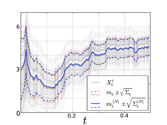
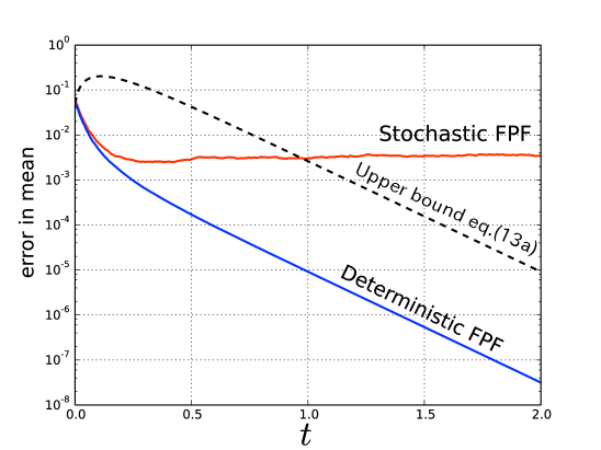
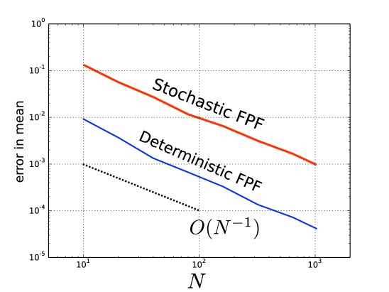
Figure 1: Results of numerical experiment: (a) Trajectories of $N=100$ particles together with the empirical mean, the empirical variance, the (true) conditional mean, and the conditional variance for a single simulation; (b) Monte-Carlo estimate of the mean-squared error (in estimating the mean) as a function of time $t$; (c) Monte-Carlo estimate of the mean-squared error as a function of $N$. The Monte-Carlo estimates are obtained by running $M=1000$ simulations.

IV Propagation of chaos

At the initial time $t=0$, the particles $\{X_{0}^{i}\}_{i=1}^{N}$ are sampled i.i.d. from the prior distribution. In any finite-$N$ implementation of the filter, the i.i.d. property is destroyed for $t>0$ because of the interactions: For the linear FPFs (5) and (7), the interaction terms are a function of the empirical mean $m^{(N)}_{t}$ and the empirical covariance $\Sigma^{(N)}_{t}$. Since these terms depend upon all the particles, the $i^{\text{th}}$ particle in the population is coupled to/interacts with (the randomness of) all other particles. Even though the particles are no longer i.i.d for any finite choice of $N$, one (formally) expects the particles to become approximately i.i.d (in a sense that needs to be made precise) for large $N$. Intuitively, this is because as $N\to\infty$, $m^{(N)}_{t}\to m_{t}$ and $\Sigma^{(N)}_{t}\to\Sigma_{t}$. And for the limiting mean-field model, the particles are i.i.d for $t>0$ provided they are i.i.d. at the initial time $t=0$. The phenomenon is referred to as the propagation of chaos whereby the chaos (i.i.d property of the population) propagates through time.

The mathematical definitions are as follows: Denote $E:=\mathbb{R}^{d}\times[0,\infty)$. Let $\mu_{N}$ be the probability measure on $E^{N}$ associated with the process $(X^{1},\ldots,X^{N})$. Let $\bar{\mu}$ be the probability measure on $E$ associated with the mean-field solution $\bar{X}$. Then $\mu_{N}$ is said to be $\bar{\mu}$-chaotic if

$$\pi_{k}\mu_{N}\overset{\text{weak}}{\longrightarrow}\bar{\mu}^{(k)}\quad\text{as}\quad N\to\infty$$

where $\pi_{k}\mu_{N}$ is the $k$-marginal distribution, $\bar{\mu}^{(k)}$ is the $k$-fold product, and the convergence is in the weak sense. A somewhat easier formulation of this condition appears in [26, Proposition 2.2] as

$$\lim_{N\to\infty}{\sf E}\left[\left|\frac{1}{N}\sum_{i=1}^{N}f(X^{i})-{\sf E}[f(\bar{X})]\right|^{2}\right]=0$$ (14)

for all bounded functionals $f:E\to\mathbb{R}$.

Remark 6

Some difficulties in carrying out the propagation of chaos analysis for the FPF are as follows: (i) The drift term in the evolution equation for the covariance is not Lipschitz; For the stochastic FPF (5), the noise terms (the martingale $M_{t}$) depend upon the state. In our analysis, we circumvent some of these difficulties by limiting to the scalar ($d=1$) case where explicit solution of the covariance is available. As was the case in Sec. III-B, we focus on the deterministic FPF where the terms due to the process noise are not present. Even in this special case, we show the convergence for the marginal distribution only for fixed time $t>0$. That is, we show

$$\lim_{N\to\infty}{\sf E}\left[\left|\frac{1}{N}\sum_{i=1}^{N}f(X^{i}_{t})-{\sf E}[f(\bar{X}_{t})]\right|^{2}\right]=0$$ (15)

for all bounded functions $f:\mathbb{R}^{d}\to\mathbb{R}$. Extension to estimates that are uniform in time in the general settings is a subject of continuing work.

Derivation of error estimates involve construction of $N$ independent copies of the mean-field equation (4) corresponding to the deterministic FPF (7). Consistent with our convention to denote mean-field variables with a bar, the stochastic processes are denoted as $\{\bar{X}_{t}^{i}:1\leq i\leq N\}$ where $\bar{X}^{i}_{t}$ denotes the state of the $i^{\text{th}}$ particle at time $t$. The particle evolves according to the mean-field equation (4) as

$$\,\mathrm{d}\bar{X}^{i}_{t} =A\bar{m}_{t}\,\mathrm{d}t+\bar{{\sf K}}_{t}(\,\mathrm{d}Z_{t}-C{\bar{m}_{t}}\,\mathrm{d}t)+\bar{G}_{t}(\bar{X}_{t}^{i}-\bar{m}_{t})\$$ (16)

where $\bar{{\sf K}}_{t}=\bar{\Sigma}_{t}C^{\top}$ is the Kalman gain and the initial condition $\bar{X}^{i}_{0}=X^{i}_{0}$ – the initial condition of the $i^{\text{th}}$ particle in the finite-$N$ FPF (7). The mean-field process $\bar{X}^{i}_{t}$ is thus coupled to $X^{i}_{t}$ through the initial condition. The following Proposition characterizes the error between $X^{i}_{t}$ and $\bar{X}^{i}_{t}$ (the estimate is essential for the propagation of chaos analysis). The proof appears in the Appendix -C.

Proposition 3

Consider the stochastic processes $X^{i}_{t}$ and $\bar{X}^{i}_{t}$ whose evolution is defined according to the deterministic FPF (7) and its mean-field model (16), respectively. The initial condition $X_{0}^{i}\stackrel{{\scriptstyle\text{i.i.d}}}{{\sim}}{\cal N}(m_{0},\Sigma_{0})$ for $i=1,2,\ldots,N$ and the dimension $d=1$. Then under Assumptions (I)-(II):

• The explicit solution is given as

  $$X^{i}_{t} =m^{(N)}_{t}+\left(\frac{\Sigma^{(N)}_{t}}{\Sigma^{(N)}_{0}}\right)^{{\mathchoice{\genfrac{}{}{}{1}{1}{2}}{\genfrac{}{}{}{2}{1}{2}}{\genfrac{}{}{}{3}{1}{2}}{\genfrac{}{}{}{4}{1}{2}}}}(X^{i}_{0}-m^{(N)}_{0})$$

  $$\bar{X}^{i}_{t} =m_{t}+\left(\frac{\Sigma_{t}}{\Sigma_{0}}\right)^{\mathchoice{\genfrac{}{}{}{1}{1}{2}}{\genfrac{}{}{}{2}{1}{2}}{\genfrac{}{}{}{3}{1}{2}}{\genfrac{}{}{}{4}{1}{2}}}(X^{i}_{0}-m_{0})$$

• For a fixed $t>0$, in the limit as $N\to\infty$

  $${\sf E}[|X^{i}_{t}-\bar{X}^{i}_{t}|^{2}]\leq\frac{\text{(const.)}}{{N}}$$ (18)

The estimate (18) is used to prove the following important result that the empirical distribution of the particles in the linear FPF converges weakly to the true posterior distribution. Its proof appears in the Appendix -C.

Corollary 1

Consider the linear filtering problem (1a)-(1b) and the finite-$N$ deterministic FPF (7). The initial condition $X_{0}^{i}\stackrel{{\scriptstyle\text{i.i.d}}}{{\sim}}{\cal N}(m_{0},\Sigma_{0})$ for $i=1,2,\ldots,N$ and the dimension $d=1$. Under Assumptions (I) and (II), for any Lipschitz function $f:\mathbb{R}^{d}\to\mathbb{R}$, in the asymptotic limit as $N\to\infty$

$${\sf E}\left[\left|\frac{1}{N}\sum_{i=1}^{N}f(X^{i}_{t})-{\sf E}[f(X_{t})|{\cal Z}_{t}]\right|^{2}\right]\leq\frac{\text{(const.)}}{{N}}$$

-A Derivation of evolution equations in Sec. III-A

(A) Finite-$N$ stochastic FPF: Consider Eq. (5) for the $i^{\text{th}}$ particle. Summing up over the index $i=1,\ldots,N$ and dividing by $N$, Eq. (11a) for the mean is obtained. To obtain (11b), first define $\xi^{i}_{t}:=X^{i}_{t}-m^{(N)}_{t}$. Therefore,

$$\,\mathrm{d}\xi^{i}_{t}=(A-\frac{1}{2}\mathsf{K}^{(N)}_{t}C)\xi^{i}_{t}\,\mathrm{d}t+\sigma_{B}\,\mathrm{d}B^{i}_{t}-\frac{1}{N}\sum_{j=1}^{N}\sigma_{B}\,\mathrm{d}B^{j}_{t}$$

and

$$\,\mathrm{d}(\xi^{i}_{t}{\xi^{i}_{t}}^{\top})= (A-\frac{1}{2}\mathsf{K}^{(N)}_{t}C)\xi^{i}_{t}{\xi^{i}_{t}}^{\top}\,\mathrm{d}t+\xi^{i}_{t}{\xi^{i}_{t}}^{\top}(A-\frac{1}{2}\mathsf{K}^{(N)}_{t}C)^{\top}\,\mathrm{d}t$$

$$+\frac{N-1}{N}\sigma_{B}\sigma_{B}^{\top}\,\mathrm{d}t+\xi^{i}_{t}(\,\mathrm{d}B_{t}^{i}-\frac{1}{N}\sum_{j=1}^{N}\,\mathrm{d}B^{j}_{t})^{\top}\sigma_{B}^{\top}$$

$$+\sigma_{B}(\,\mathrm{d}B_{t}^{i}-\frac{1}{N}\sum_{j=1}^{N}\,\mathrm{d}B^{j}_{t}){\xi^{i}_{t}}^{\top}$$

Summing over $i=1,\ldots,N$ and dividing by $(N-1)$ gives

$$\,\mathrm{d}\Sigma^{(N)}_{t}= (A-\frac{1}{2}{\sf K}_{t}^{(N)}C)\Sigma^{(N)}_{t}\,\mathrm{d}t+\Sigma^{(N)}_{t}(A-\frac{1}{2}{\sf K}_{t}^{(N)}C)^{\top}\,\mathrm{d}t$$

$$+\sigma_{B}\sigma_{B}^{\top}\,\mathrm{d}t+\frac{1}{N-1}\sum_{i=1}^{N}\xi^{i}_{t}{\,\mathrm{d}B^{i}_{t}}^{\top}\sigma_{B}^{\top}+\frac{1}{N-1}\sum_{i=1}^{N}\sigma_{B}\,\mathrm{d}B^{i}_{t}{\xi^{i}_{t}}^{\top}$$

which is Eq. (11b) for the covariance.

(B) Finite-$N$ deterministic FPF: Eq. (7) is obtained as before by summing up Eq. (7) for the $i^{\text{th}}$ particle from $i=1,\ldots,N$. The equation for the empirical mean is simply obtained by summing up the equations (7) for $i=1,\ldots,N$. To obtain the equation for the empirical covariance, first define $\xi^{i}_{t}:=X^{i}_{t}-m^{(N)}_{t}$. Therefore, $\,\mathrm{d}\xi^{i}_{t}=G_{t}^{(N)}\xi^{i}_{t}\,\mathrm{d}t$ and

$$\,\mathrm{d}(\xi^{t}{\xi^{i}_{t}}^{\top})=G_{t}^{(N)}\xi^{i}_{t}{\xi^{i}_{t}}^{\top}\,\mathrm{d}t+\xi^{i}_{t}{\xi^{i}_{t}}^{\top}{G_{t}^{(N)}}^{\top}\,\mathrm{d}t$$

Summing over $i=1,\ldots,N$ and dividing by $(N-1)$ gives

$$\frac{\,\mathrm{d}\Sigma^{(N)}_{t}}{\,\mathrm{d}t} =G_{t}^{N}\Sigma^{(N)}_{t}+\Sigma^{(N)}_{t}{G_{t}^{(N)}}^{\top}$$

which is Eq. (12b) for the covariance.

It is noted that $G_{t}^{(N)}$ is well-defined because $\Sigma^{(N)}_{0}$ and thus $\Sigma^{(N)}_{t}$ is invertible because of Assumption (II).

-B Proof of the Prop. 2

Since the equations for the empirical mean (12a) and the empirical covariance (12b) are identical to the Kalman filter (2a)-(2b), the a.s. convergence of mean and variance follows from the filter stability theory (see Theorem 1). In the following, mean-squared estimates are derived for the large-$N$ limit. We begin with the scalar ($d=1$) case:

Scalar case: The explicit solution of (12b) is given by

$$\Sigma^{(N)}_{t}=\Sigma_{\infty}+\frac{e^{-2\lambda_{0}t}}{\frac{1}{\Sigma^{(N)}_{0}-\Sigma_{\infty}}+\frac{C^{2}}{2\lambda_{0}}(1-e^{-2\lambda_{0}t})}=:f(\Sigma^{(N)}_{0},t)$$ (19)

where $\lambda_{0}=(A^{2}+\sigma_{B}^{2}C^{2})^{\mathchoice{\genfrac{}{}{}{1}{1}{2}}{\genfrac{}{}{}{2}{1}{2}}{\genfrac{}{}{}{3}{1}{2}}{\genfrac{}{}{}{4}{1}{2}}}$ and $\Sigma_{\infty}=\frac{A+\lambda_{0}}{C^{2}}$. The function $f(x,t)$ is Lipschitz with respect to $x$ with Lischitz constant $\beta e^{-2\lambda_{0}t}$ where $\beta=(\frac{2\lambda_{0}}{\lambda_{0}-A})^{2}$. Therefore

$$|\Sigma^{(N)}_{t}-\Sigma_{t}|\leq\beta e^{-2\lambda_{0}t}|\Sigma^{(N)}_{0}-\Sigma_{0}|$$

Hence

$${\sf E}[|\Sigma^{(N)}_{t}-\Sigma_{t}|^{2}] \leq\beta^{2}e^{-4\lambda_{0}t}{\sf E}[|\Sigma^{(N)}_{0}-\Sigma_{0}|^{2}]$$

$$\leq\beta^{2}e^{-4\lambda_{0}t}\frac{{\sf E}[|X_{0}-m_{0}|^{4}]-\Sigma^{2}_{0}}{N}+O(\frac{1}{N^{2}})$$

which gives the result (13b) for the scalar case.

The estimate (13a) for the mean is obtained next. Define $\delta m_{t}:=m^{(N)}_{t}-m_{t}$ and $\delta\Sigma_{t}:=\Sigma^{(N)}_{t}-\Sigma_{t}$. Using-(12a) and (2a),

$$\,\mathrm{d}\delta m_{t}= (A-C^{2}\Sigma^{(N)}_{t})\delta m_{t}\,\mathrm{d}t+\delta\Sigma_{t}C\,\mathrm{d}I_{t}$$

where $\,\mathrm{d}I_{t}:=\,\mathrm{d}Z_{t}-Cm_{t}\,\mathrm{d}t$ is the innovation process. Therefore,

$$\delta m_{t}=e^{\int_{0}^{t}(A-C^{2}\Sigma^{(N)}_{s})\,\mathrm{d}s}\delta m_{0}+\int_{0}^{t}e^{\int_{s}^{t}(A-C^{2}\Sigma^{(N)}_{\tau})\,\mathrm{d}\tau}C\delta\Sigma_{s}\,\mathrm{d}I_{s}$$

Squaring the expression and taking the expectation yields

$${\sf E}[|\delta m_{t}|^{2}] =e^{2\int_{0}^{t}(A-C^{2}\Sigma_{s})\,\mathrm{d}s}{\sf E}[|\delta m_{0}|^{2}]$$

$$+\int_{0}^{t}e^{2\int_{s}^{t}(A-C^{2}\Sigma_{\tau})\,\mathrm{d}\tau}C^{2}{\sf E}[|\delta\Sigma_{s}|^{2}]\,\mathrm{d}t$$

where we have used the fact that the innovation process $I_{t}$ is a Wiener process [30, Lemma 5.6]. Then using the bound

$$\int_{s}^{t} (A-C^{2}\Sigma^{(N)}_{s})\,\mathrm{d}s$$

$$=-\lambda_{0}(t-s)+\log(\frac{1+(\Sigma^{(N)}_{0}-\Sigma_{\infty})\frac{C^{2}}{2\lambda_{0}}(1-e^{-2\lambda_{0}s})}{1+(\Sigma^{(N)}_{0}-\Sigma_{\infty})\frac{C^{2}}{2\lambda_{0}}(1-e^{-2\lambda_{0}t})})$$

$$\leq-\lambda_{0}(t-s)+\frac{1}{2}|\log(\beta)|$$

and ${\sf E}[|\delta\Sigma_{s}|^{2}]\leq\beta^{2}e^{-4\lambda_{0}t}{\sf E}[|\delta\Sigma_{0}|^{2}]$ we obtain

$${\sf E}[|\delta m_{t}|^{2}]\leq e^{-2\lambda_{0}t+|\log(\beta)|}{\sf E}[|\delta m_{0}|^{2}]$$

$$+C^{2}\beta^{2}e^{-2\lambda_{0}t+|\log(\beta)|}\frac{1}{2\lambda_{0}}(1-e^{-2\lambda_{0}t}){\sf E}[|\delta\Sigma_{0}|^{2}]$$

The mean-squared estimate (13a) for the mean in the scalar case follows from noting ${\sf E}[|\delta m_{0}|^{2}]=\frac{{\sf E}[|X_{0}-m_{0}|^{2}]}{N}$ and ${\sf E}[|\delta\Sigma_{0}|^{2}]\leq\frac{{\sf E}[|X_{0}-m_{0}|^{4}}{N}$.

Vector case: The explicit solution of the Riccati equation in the vector case is given by [3, pp. 149]

$$\Sigma^{(N)}_{t}=\Sigma_{\infty}+e^{F_{\infty}t}D_{t}^{-1}e^{F_{\infty}^{\top}t}=:f(\Sigma^{(N)}_{0},t)$$ (20)

where $F_{\infty}:=A-\Sigma_{\infty}C^{\top}C$, and

$$D_{t} :=(\Sigma^{(N)}_{0}-\Sigma_{\infty})^{-1}+\int_{0}^{t}e^{F_{\infty}^{\top}s}C^{\top}Ce^{F_{\infty}s}\,\mathrm{d}s$$

The function $f(x,t)$ is Lipschitz with respect to to $x$ with Lipschitz constant $\beta_{d}e^{-2\lambda_{0}t}$ where $\beta_{d}:=\sup_{\Sigma^{(N)}_{0}}\|(D_{t}(\Sigma^{(N)}_{0}-\Sigma_{\infty}))^{-1}\|_{s}^{2}$ Therefore,

$$\|\Sigma^{(N)}_{0}-\Sigma_{t}\|_{F}\leq \beta_{d}e^{-2\lambda_{0}t}\|\Sigma^{(N)}_{0}-\Sigma_{0}\|_{F}$$

Squaring both sides and taking expectation gives the covariance error estimate:

$${\sf E}[\|\Sigma^{(N)}_{t}-\Sigma_{t}\|_{F}^{2}]\leq\beta_{d}^{2}e^{-4\lambda_{0}t}\frac{{\sf E}[|X_{0}-m_{0}|^{4}]-\text{Tr}(\Sigma_{0}^{2})}{N}+O(\frac{1}{N^{2}})$$

where we have used ${\sf E}[\|\Sigma^{(N)}_{0}-\Sigma_{0}\|_{F}^{2}]=\frac{{\sf E}[|X_{0}-m_{0}|^{4}]-\text{Tr}(\Sigma_{0}^{2})}{N}+O(N^{-2})$.

The procedure for obtaining the error estimate for the mean is also as before. As in the scalar case,

$$\delta m_{t}=\Phi_{t,0}\delta m_{0}+\int_{0}^{t}\Phi_{t,s}\delta\Sigma_{s}C^{\top}\,\mathrm{d}I_{s}$$

where $\Phi_{t,s}$ is the state transition matrix for $F^{(N)}_{t}=A-\Sigma^{(N)}_{t}C^{\top}C$. The expected norm-squared of $\delta m_{t}$ is

$${\sf E}[|\delta m_{t}|^{2}]= {\sf E}[\delta m_{0}^{\top}\Phi_{t,0}^{\top}\Phi_{t,0}\delta m_{0}]$$

$$+\int_{0}^{t}\text{Tr}(C\delta\Sigma_{s}\Phi_{t,s}^{\top}\Phi_{t,s}\delta\Sigma_{s}C^{\top})\,\mathrm{d}s$$ (21)

where we used the fact that the innovation process $I_{t}$ is a Wiener process. Expressing $F_{t}^{(N)}=F_{\infty}-e^{F_{\infty}t}D_{t}^{-1}e^{F^{\top}_{\infty}t}C^{\top}C$, its spectral norm is bounded as $\|F_{t}^{(N)}\|_{s}\leq-\lambda_{0}+e^{-2\lambda_{0}t}2\lambda_{0}c_{0}$ where $c_{0}:=\frac{1}{2\lambda_{0}}\|C^{\top}C\|_{s}\sup_{\Sigma^{(N)}_{0}}\|D_{t}^{-1}\|_{s}$. Therefore $\|\Phi_{t,s}\|_{s}\leq e^{-\lambda_{0}t+c_{0}}$. Use this inequality in (21) to conclude

$${\sf E}[|\delta m_{t}|^{2}] =e^{-2\lambda_{0}t+2c_{0}}{\sf E}[|\delta m_{0}|^{2}]+$$

$$+e^{-2\lambda_{0}t+2c_{0}}\frac{1-e^{-2\lambda_{0}t}}{2\lambda_{0}}\|CC^{\top}\|_{s}\beta_{d}^{2}{\sf E}[\|\delta\Sigma_{0}^{2}\|_{F}^{2}]$$

The error bound (13a) follows from noting, as also in the scalar case, ${\sf E}[|\delta m_{0}|^{2}]=\frac{1}{N}{\sf E}[|X_{0}-m_{0}|^{2}]$ and ${\sf E}[\|\delta\Sigma_{0}\|_{F}^{2}]\leq\frac{{\sf E}[|X_{0}-m_{0}|^{4}}{N}$.

-C Proofs of the Prop. 3 and Cor. 1

Proof:

Part (i): Use the decomposition

$$X^{i}_{t}=m^{(N)}_{t}+\xi^{i}_{t},\quad\bar{X}^{i}_{t}=m_{t}+\bar{\xi}^{i}_{t}$$

Recall that

$$\,\mathrm{d}{\xi}^{i}_{t} =G_{t}^{(N)}{\xi}^{i}_{t}\,\mathrm{d}t,\quad\,\mathrm{d}\bar{\xi}^{i}_{t}=G_{t}\bar{\xi}^{i}_{t}\,\mathrm{d}t$$

Hence, for the scalar case

$${\xi}^{i}_{t} =e^{\int_{0}^{t}G_{s}^{(N)}\,\mathrm{d}s}{\xi}^{i}_{0},\quad\bar{\xi}^{i}_{t}=e^{\int_{0}^{t}G_{s}\,\mathrm{d}s}\bar{\xi}^{i}_{0}$$

By definition, $G^{(N)}_{t}$ and $G_{t}$ satisfy

$$2\Sigma^{(N)}_{t}G_{t}=\frac{\,\mathrm{d}\Sigma^{(N)}_{t}}{\,\mathrm{d}t},\quad 2\Sigma_{t}G_{t}=\frac{\,\mathrm{d}\Sigma_{t}}{\,\mathrm{d}t}$$

Therefore

$$\int_{0}^{t}G^{(N)}_{s}\,\mathrm{d}s=\frac{1}{2}\log(\frac{\Sigma^{(N)}_{t}}{\Sigma^{(N)}_{0}}),\quad\int_{0}^{t}G_{s}\,\mathrm{d}s=\frac{1}{2}\log(\frac{\Sigma_{t}}{\Sigma_{0}})$$

which concludes the result for part (i) of the Proposition.

Part (ii): Use the triangle inequality to conclude

$${\sf E}[|X^{i}_{t}-\bar{X}^{i}_{t}|^{2}]^{\frac{1}{2}}\leq{\sf E}[|\xi^{i}_{t}-\bar{\xi}^{i}_{t}|^{2}]^{\frac{1}{2}}+{\sf E}[|m^{(N)}_{t}-m_{t}|^{2}]^{\frac{1}{2}}$$

The error between $m^{(N)}_{t}$ and $m_{t}$ is already obtained as part of the Prop. 2 given by (13a). Using the explicit solutions in part (i), the other term is the $L^{2}$-norm of

$$\xi^{i}_{t}-\bar{\xi}^{i}_{t} =\underbrace{(\left(\frac{\Sigma^{(N)}_{t}}{\Sigma^{(N)}_{0}}\right)^{\frac{1}{2}}-\left(\frac{\Sigma_{t}}{\Sigma_{0}}\right)^{\frac{1}{2}}){\xi}^{i}_{0}}_{\text{(I)}}+\underbrace{\left(\frac{\Sigma_{t}}{\Sigma_{0}}\right)^{\frac{1}{2}}(\xi^{i}_{0}-\bar{\xi}_{0})}_{\text{(II)}}$$

A bound on the second term (II) is obtained as follows:

$${\sf E}\left[\frac{\Sigma_{t}}{\Sigma_{0}}|\xi^{i}_{0}-\bar{\xi}_{0}|^{2}\right]\leq\frac{\Sigma_{t}}{\Sigma_{0}}{\sf E}\left[|\xi^{i}_{0}-\bar{\xi}_{0}|^{2}\right] =\frac{\Sigma_{t}}{\Sigma_{0}}{\sf E}\left[|m^{(N)}_{0}-m_{0}|^{2}\right]$$

$$=\frac{\Sigma_{t}}{\Sigma_{0}}\frac{{\sf E}[|X_{0}-m_{0}|^{2}]}{N}$$

where we used the identity $\xi^{i}_{0}+m^{(N)}_{0}=\bar{\xi}^{i}_{0}+m_{0}$ because $X^{i}_{t}=\bar{X}^{i}_{t}$. The bound the first term (I) is involved. Define $g(x,t):=\sqrt{\frac{f(x,t)}{x}}$ where $f$ is defined in (19). We are interested in obtaining a bound on ${\sf E}[|g(\Sigma^{(N)}_{0},t)-g(\Sigma_{0},t)|^{2}{\xi^{i}_{0}}^{2}]$. Denote $r(\omega):=g(\Sigma^{(N)}_{0}(\omega),t)-g(\Sigma_{0},t)$ and express

$$r=r\mathds{1}_{S}+r\mathds{1}_{S^{c}}$$

where the event $S:=\{\omega\;:\;\Sigma^{(N)}_{0}(\omega)\geq\frac{1}{2}\Sigma_{0}\}$. On $S$, the function $g(x,t)$ is Lipschitz with respect to $x$ with Lipschitz constant $L_{g}=\frac{\beta e^{-2\lambda_{0}t}}{2\min(\Sigma_{0},\Sigma_{\infty})}+\frac{2\sqrt{\Sigma_{\infty}}}{\min(\Sigma_{\infty},\Sigma_{0})^{3/2}}$. On the complement $S^{c}$:

$${\sf E}[r^{2}{\xi^{i}_{0}}^{2}\mathds{1}_{S^{c}}] \leq 2{\sf E}\left[\frac{\Sigma^{(N)}_{t}}{\Sigma^{(N)}_{0}}{\xi^{i}_{0}}^{2}\mathds{1}_{S^{c}}\right]+2{\sf E}\left[\frac{\Sigma_{t}}{\Sigma_{0}}{\xi^{i}_{0}}^{2}\mathds{1}_{S^{c}}\right]$$

$$\leq 2N{\sf E}[\Sigma^{(N)}_{t}\mathds{1}_{S^{c}}]+2N\frac{\Sigma_{t}}{\Sigma_{0}}{\sf E}[\Sigma^{(N)}_{0}\mathds{1}_{S^{c}}]$$

$$\leq 4N(\Sigma_{\infty}+\Sigma_{0}){\sf P}({S^{c}})$$

where we used the bound ${\xi^{i}_{0}}^{2}\leq N\Sigma^{(N)}_{0}$. For large $N$, the probability of the event $S^{c}$ exponentially decays with $N$ (Chernoff bound). As a result, for large $N$, the bound is obtained in terms of the Lipschitz constant:

$${\sf E}[|g(\Sigma^{(N)}_{0},t)-g(\Sigma_{0},t)|^{2}{\xi^{i}_{0}}^{2}] \leq L_{g}^{2}{\sf E}\left[|\Sigma^{(N)}_{0}-\Sigma_{0}|^{2}|{\xi}^{i}_{0}|^{2}\right]$$

$$\leq L_{g}^{2}{\sf E}\left[|\Sigma^{(N)}_{0}-\Sigma_{0}|^{4}\right]^{\frac{1}{2}}{\sf E}\left[|{\xi}^{i}_{0}|^{4}\right]^{\frac{1}{2}}$$

$$\leq L_{g}^{2}\frac{{\sf E}[|X_{0}-m_{0}|^{4}]^{\frac{3}{2}}}{{N}}+O(N^{-2})$$

where we used the Lipschitz property in the first step, the Cauchy-Schwarz inequality in the second step, and ${\sf E}[|\Sigma^{(N)}_{0}-\Sigma_{0}|^{4}]^{\frac{1}{4}}=\frac{{\sf E}[|X_{0}-m_{0}|^{4}]^{\frac{1}{2}}}{\sqrt{N}}+O(N^{-1})$ in the last step.  

Proof:

Using the triangle inequality,

$${\sf E}[|\frac{1}{N}\sum_{i=1}^{N}f(X^{i}_{t})-\hat{f}|^{2}]^{1/2}\leq {\sf E}[|\frac{1}{N}\sum_{i=1}^{N}f(X^{i}_{t})-\frac{1}{N}\sum_{i=1}^{N}f(\bar{X}^{i}_{t})|^{2}]^{1/2}$$

$$+{\sf E}[|\frac{1}{N}\sum_{i=1}^{N}f(\bar{X}^{i}_{t})-\hat{f}|^{2}]^{1/2}$$

where $\hat{f}:={\sf E}[f(X_{t})|{\cal Z}_{t}]$. The second term is given by

$${\sf E}[|\frac{1}{N}\sum_{i=1}^{N}f(\bar{X}^{i}_{t})-\hat{f}|^{2}]^{1/2}=\frac{\text{Var}(f)}{\sqrt{N}}$$

because $\bar{X}^{i}_{t}$ are i.i.d with distribution equal to the conditional distribution. It only remains to bound the first term:

$${\sf E}[|\frac{1}{N}\sum_{i=1}^{N}f(X^{i}_{t}) -\frac{1}{N}\sum_{i=1}^{N}f(\bar{X}^{i}_{t})|^{2}]\leq\frac{1}{N}\sum_{i=1}^{N}{\sf E}[|f(X^{i}_{t})-f(\bar{X}^{i}_{t})|^{2}]$$

$$\leq\frac{\text{(const.)}}{N}\sum_{i=1}^{N}{\sf E}[|X^{i}_{t}-\bar{X}^{i}_{t}]|^{2}]\leq\frac{\text{(const.)}}{N}$$

where we used Jensen’s inequality in the first step, the Lipschitz property of $f$ in the second step, and the estimate (18) in the last step.

References

- [1] K. Bergemann and S. Reich. An ensemble Kalman-Bucy filter for continuous data assimilation. Meteorologische Zeitschrift, 21(3):213–219, 2012.
- [2] K Berntorp. Feedback particle filter: Application and evaluation. In 18th Int. Conf. Information Fusion, Washington, DC, 2015.
- [3] R. W. Brockett. Finite dimensional linear systems. John Wiley and Sons, New York, 1970.
- [4] D. Crisan and J. Xiong. Approximate McKean-Vlasov representations for a class of SPDEs. Stochastics, 82(1):53–68, 2010.
- [5] F. Daum and J. Huang. Particle flow for nonlinear filters with log-homotopy. In Proc. SPIE, volume 6969, pages 696918–696918, 2008.
- [6] F. Daum, J. Huang, and A. Noushin. Generalized Gromov method for stochastic particle flow filters. In SPIE Defense+ Security, pages 102000I–102000I. International Society for Optics and Photonics, 2017.
- [7] J. de Wiljes, S. Reich, and W. Stannat. Long-time stability and accuracy of the ensemble Kalman-Bucy filter for fully observed processes and small measurement noise. arXiv preprint arXiv:1612.06065, 2016.
- [8] P. Del Moral. Feynman-Kac formulae. In Feynman-Kac Formulae, pages 47–93. Springer, 2004.
- [9] P. Del Moral, A. Kurtzmann, and J. Tugaut. On the stability and the uniform propagation of chaos of a class of extended ensemble Kalman–Bucy filters. SIAM Journal on Control and Optimization, 55(1):119–155, 2017.
- [10] P. Del Moral and J. Tugaut. On the stability and the uniform propagation of chaos properties of ensemble Kalman-Bucy filters. arXiv preprint arXiv:1605.09329, 2016.
- [11] M. Huang, P. E. Caines, and R. P. Malhame. Large-population cost-coupled LQG problems with nonuniform agents: Individual-mass behavior and decentralized -Nash equilibria. IEEE transactions on automatic control, 52(9):1560–1571, 2007.
- [12] R. E Kalman and R. S Bucy. New results in linear filtering and prediction theory. Journal of basic engineering, 83(1):95–108, 1961.
- [13] D. Kelly, K. JH. Law, and A. M. Stuart. Well-posedness and accuracy of the ensemble Kalman filter in discrete and continuous time. Nonlinearity, 27(10):2579, 2014.
- [14] E. Kwiatkowski and J. Mandel. Convergence of the square root ensemble kalman filter in the large ensemble limit. SIAM/ASA Journal on Uncertainty Quantification, 3(1):1–17, 2015.
- [15] J.-M. Lasry and P.-L. Lions. Mean field games. Japan. J. Math., 2:229–260, 2007.
- [16] R. S. Laugesen, P. G. Mehta, S. P. Meyn, and M. Raginsky. Poisson’s equation in nonlinear filtering. SIAM Journal on Control and Optimization, 53(1):501–525, 2015.
- [17] F. Le Gland, V. Monbet, and V. Tran. Large sample asymptotics for the ensemble Kalman filter. PhD thesis, INRIA, 2009.
- [18] H. P. McKean. A class of markov processes associated with nonlinear parabolic equations. Proceedings of the National Academy of Sciences of the United States of America, 56(6):1907–1911, 1966.
- [19] H. P. McKean. A class of Markov processes associated with nonlinear parabolic equations. Proceedings of the National Academy of Sciences, 56(6):1907–1911, 1966.
- [20] D. Ocone and E. Pardoux. Asymptotic stability of the optimal filter with respect to its initial condition. SIAM Journal on Control and Optimization, 34(1):226–243, 1996.
- [21] S. T. Rachev and L. Rüschendorf. Mass Transportation Problems: Volume I: Theory, volume 1. Springer Science & Business Media, 1998.
- [22] S. Reich. A dynamical systems framework for intermittent data assimilation. BIT Numerical Mathematics, 51(1):235–249, 2011.
- [23] P. M. Stano. Nonlinear State and Parameter Estimation for Hopper Dredgers. PhD thesis, Ph. D. dissertation). Delft University of Technology, 2013.
- [24] P. M. Stano, A. K. Tilton, and R. Babuska. Estimation of the soil-dependent time-varying parameters of the hopper sedimentation model: The FPF versus the BPF. Control Engineering Practice, 24:67–78, 2014.
- [25] S. C. Surace, A. Kutschireiter, and J.-P. Pfister. How to avoid the curse of dimensionality: scalability of particle filters with and without importance weights. ArXiv e-prints, March 2017.
- [26] A. Sznitman. Topics in propagation of chaos. Ecole d’Eté de Probabilités de Saint-Flour XIX—1989, pages 165–251, 1991.
- [27] A. Taghvaei, J de Wiljes, P. G. Mehta, and S. Reich. Kalman filter and its modern extensions for the continuous-time nonlinear filtering problem. ASME Journal of Dynamic Systems, Measurement, and Control, 2017. To Appear.
- [28] A. Taghvaei and P. G. Mehta. An optimal transport formulation of the linear feedback particle filter. In American Control Conference (ACC), 2016, pages 3614–3619. IEEE, 2016.
- [29] A. K. Tilton, S. Ghiotto, and P. G. Mehta. A comparative study of nonlinear filtering techniques. In Proc. Int. Conf. on Inf. Fusion, pages 1827–1834, Istanbul, Turkey, July 2013.
- [30] J. Xiong. An introduction to stochastic filtering theory, volume 18 of Oxford Graduate Texts in Mathematics. Oxford University Press, 2008.
- [31] T. Yang, R. S. Laugesen, P. G. Mehta, and S. P. Meyn. Multivariable feedback particle filter. Automatica, 71:10–23, 2016.
- [32] T. Yang, P. G. Mehta, and S. P. Meyn. Feedback particle filter. IEEE Transactions on Automatic Control, 58(10):2465–2480, October 2013.