Proceedings of the Fifth Annual LHCP ATL-PHYS-PROC-2017-233

Study of $b\to s\ell\ell$ decays at ATLAS

Marcella Bona

On behalf of the ATLAS Collaboration,
School of Physics and Astronomy
Queen Mary University of London, London, UK

ABSTRACT

The study of flavour-changing neutral currents (FCNC) gives access to important tests of the Standard Model (SM) and allows to search for hints of beyond the SM phenomena. We present here the study of the very rare decays $B^{0}\to\mu^{+}\mu^{-}$ and $B_{s}^{0}\to\mu^{+}\mu^{-}$ using data corresponding to an integrated luminosity of 25 fb^-1 of $7$ TeV and $8$ TeV proton–proton collisions collected with the ATLAS detector during the LHC Run 1. For $B^{0}$, an upper limit on the branching fraction is set at BR$(B^{0}\to\mu^{+}\mu^{-})<4.2\times 10^{-10}$ at 95% confidence level. For $B^{0}_{s}$, the branching fraction BR$(B^{0}_{s}\to\mu^{+}\mu^{-})=(0.9^{+1.1}_{-0.8})\times 10^{-9}$ is measured. The results are consistent with the SM expectation with a p-value of 4.8%, corresponding to 2.0 standard deviations. Another study sensitive to possible new physics contributions in $b\to s\ell\ell$ decays is the angular analysis of the decay $B^{0}\to K^{*}\mu^{+}\mu^{-}$. Here we present the results obtained using proton–proton collisions at $\sqrt{s}=8$ TeV from LHC data collected with the ATLAS detector. The study is based on 20.3 fb^-1 of integrated luminosity collected during 2012. Measurements of the $K^{*}$ longitudinal polarisation fraction and a set of angular parameters obtained for this decay are presented. The results are compared to a variety of theoretical predictions and found to be compatible with them.

PRESENTED AT

The Fifth Annual Conference

on Large Hadron Collider Physics

Shanghai Jiao Tong University, Shanghai, China

May 15-20, 2017

1 Introduction

Flavor-changing neutral currents (FCNC) have played a significant role in the construction of the Standard Model of particle physics (SM). These processes are forbidden at tree level in the SM, hence they need to proceed at next-to-leading order, via loops, resulting in being rare or even very rare. An important set of FCNC processes involve the transition of a $b$ quark to an $s\mu^{+}\mu^{-}$ final state mediated by electroweak box and loop diagrams. If heavy new particles exist, they may contribute to FCNC decay amplitudes, affecting the measurement of SM observables. The branching fractions of the $B^{0}\!{}_{(s)}\to\mu^{+}\mu^{-}$ decays are of particular interest because the additional helicity suppression makes them very rare and because they are accurately predicted in the SM. Also the decay $B^{0}\to K^{*}(892)\mu^{+}\mu^{-}$, where $K^{*}(892)\to K^{+}\pi^{-}$, and in particular the angular distribution of its four-body final state gives access to numerous observables sensitive to new physics. Angular observables such as the forward-backward asymmetry ($A_{\mathrm{FB}}$) should be measured as a function of the invariant mass squared of the di-lepton system ($q^{2}$), as they can be sensitive to different types of new physics introduced as FCNCs at loop level.

2 Study of the rare decays of $B^{0}_{s}$ and $B^{0}$ into muon pairs

We present here the result of a search for $B^{0}_{s}\to\mu^{+}\mu^{-}$ and $B^{0}\to\mu^{+}\mu^{-}$ decays [1] performed using $pp$ collision data corresponding to an integrated luminosity of 25 fb^-1, collected at $7$ and $8$ TeV in the full LHC Run 1 data-taking period using the ATLAS detector [2]. The SM predictions for $B^{0}\!{}_{(s)}\to\mu^{+}\mu^{-}$ decays are $\mbox{\rm BR}(B^{0}_{s}\to\mu^{+}\mu^{-})=(3.65\pm 0.23)\times 10^{-9}$ and $\mbox{\rm BR}(B^{0}\to\mu^{+}\mu^{-})=(1.06\pm 0.09)\times 10^{-10}$ [3]. The LHCb collaboration has recently reported a first single-experiment observation of $B^{0}_{s}\to\mu^{+}\mu^{-}$ obtaining $\mbox{\rm BR}(B^{0}_{s}\to\mu^{+}\mu^{-})=\left(2.8^{+0.7}_{-0.6}\right)\times 10^{-9}$ and $\mbox{\rm BR}(B^{0}\to\mu^{+}\mu^{-})=\left(3.9^{+1.6}_{-1.4}\right)\times 10^{-10}$ [4], while the first observation has been obtained by the combined analyses of the LHCb and CMS collaborations [5].

The $B^{0}_{s}\to\mu^{+}\mu^{-}$ and $B^{0}\to\mu^{+}\mu^{-}$ branching fractions are measured relative to the normalisation decay $B^{+}\to J/\psi(\to\mu^{+}\mu^{-})K^{+}$ that is abundant and has a known branching fraction. The $B^{0}\to\mu^{+}\mu^{-}$ ($B^{0}_{s}\to\mu^{+}\mu^{-}$) branching fraction can be extracted as:

$$\mbox{\rm BR}(B^{0}_{(s)}\!\to\!\mu^{+}\mu^{-})=N_{d(s)}\times\left[\mbox{\rm BR}(B^{+}\to J/\psi\,K^{+})\times\mbox{\rm BR}(J/\psi\to\mu^{+}\mu^{-})\right]\times\frac{f_{u}}{f_{d(s)}}\times\frac{1}{\mathcal{D}_{\mathrm{norm}}}\,,\\$$ (1)

$$\mbox{with}\;\;\;\;\;\;\;\;\;\mathcal{D}_{\mathrm{norm}}=\sum_{k}N^{k}_{J/\psi K^{+}}\alpha_{k}\left(\frac{\varepsilon_{\mu^{+}\mu^{-}}}{\varepsilon_{J/\psi\,K^{+}}}\right)_{k}\,,$$ (2)

where $N_{d}$ ($N_{s}$) is the $B^{0}\to\mu^{+}\mu^{-}$ ($B^{0}_{s}\to\mu^{+}\mu^{-}$) signal yield, $N_{J/\psi K^{+}}$ is the $B^{+}\to J/\psi\,K^{+}$ normalisation yield, $\varepsilon_{\mu^{+}\mu^{-}}$ and $\varepsilon_{J/\psi K^{+}}$ are the values of acceptance times efficiency, and $f_{u}/f_{d}$ ($f_{u}/f_{s}$) is the ratio of the hadronisation probabilities of a $b$-quark into $B^{+}$ and $B^{0}$ ($B^{0}_{s}$). The denominator $\mathcal{D}_{\mathrm{norm}}$ consists of a sum whose index $k$ runs over the data-taking periods and the trigger selections. The $\alpha_{k}$ parameter takes into account the different trigger prescale factors and integrated luminosities in the signal and normalisation channels. The ratio of the efficiencies corrects for reconstruction differences in each data sample $k$. Signal and reference channel events are selected with similar di-muon triggers.

The background to the $B^{0}\!{}_{(s)}\to\mu^{+}\mu^{-}$ signal originates from three main sources:

continuum background, the dominant combinatorial component, made from muons coming from uncorrelated hadron decays and characterised by a smooth di-muon invariant mass distribution. It is studied in the signal mass sidebands, and in an inclusive MC sample of semileptonic decays of $b$ and $c$ hadrons.

partially reconstructed $B\to\mu\mu X$ decays, characterised by non-reconstructed final-state particles ($X$) and thus accumulating in the low di-muon invariant mass sideband;

peaking background, due to $B^{0}\!{}_{(s)}\to h\,h^{\prime}$ decays, with both hadrons misidentified as muons.

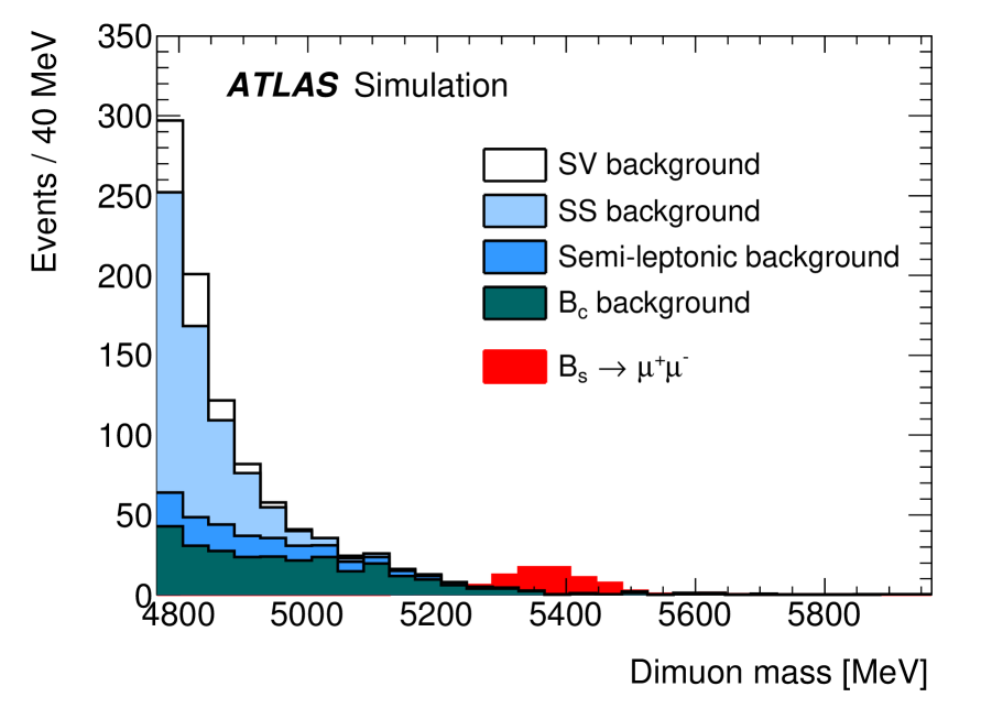
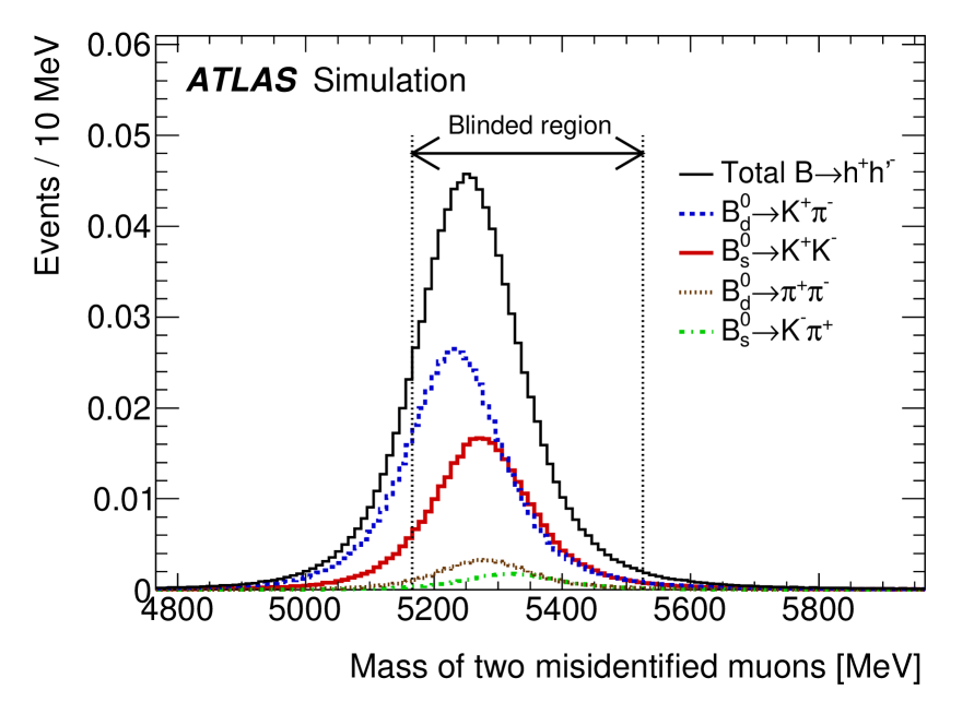
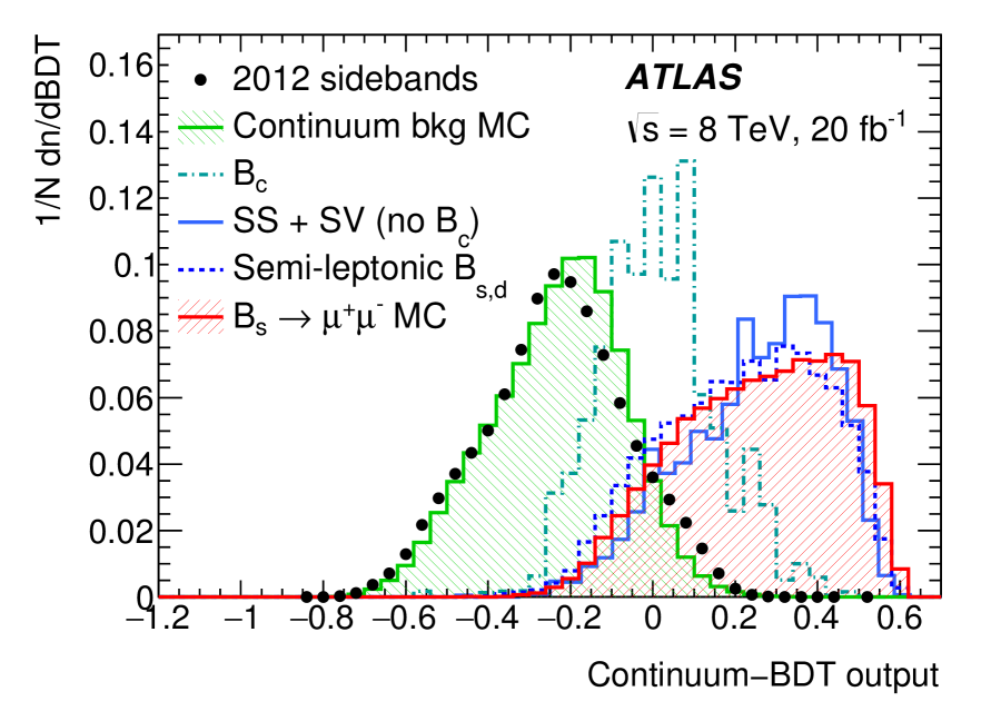
Figure 1: Left: di-muon invariant mass distribution from simulation for partially reconstructed backgrounds. Components are shown as stacked histograms, normalised according to world-averaged branching fractions. The SM expectation for the $B^{0}_{s}\to\mu^{+}\mu^{-}$ signal is also shown for comparison (non-stacked). Centre: invariant mass distribution for the peaking background $B^{0}\!{}_{(s)}\to hh^{\prime}$. Right: continuum-BDT distribution for signal and background events: signal $B^{0}\!{}_{(s)}$, partially reconstructed $B$ events (SS+SV), $B^{0}_{c}$ decays and continuum. The solid histograms are obtained from simulation, while the points represent data collected in the sidebands [1].

The partially reconstructed decays consist of several topologies: (a) same-side (SS) combinatorial background from decay cascades ($b\to c\mu\nu\to s(d)\mu\mu\nu\nu$); (b) same-vertex (SV) background from $B$ decays containing a muon pair (e.g. $B^{0}\to K^{*0}\mu\mu$, $B\to J/\psi X\to\mu\mu\mu X^{\prime}$); (c) $B_{c}$ decays (e.g. $B_{c}\to J/\psi\mu\nu\to\mu\mu\mu\nu$); (d) semileptonic $b$-hadron decays where a final-state hadron is misidentified as a muon. The latter are mainly three-body charmless decays $B^{0}\to\pi\mu\nu$, $B^{0}_{s}\to K\mu\nu$ and $\Lambda_{b}\to p\mu\nu$ and their contribution is reduced by the muon identification requirements. The MC invariant mass distributions of all these topologies are shown in the left plot in Figure 1. The peaking background is due to $B^{0}\!{}_{(s)}$ decays containing two hadrons misidentified as muons, which populate the signal region as shown in the central plot in Figure 1.

Two multivariate discriminants, implemented as BDTs, have been employed: the “fake-BDT” aims at minimising the amount of hadrons erroneously identified as muons and the “continuum-BDT” aims at discriminating against the continuum background. For the fake-muon background, the vast majority of events with hadron misidentification are due to decays in flight of kaons and pions. The fake-BDT selection is tuned for a 95% efficiency for signal muons, and the resulting misidentification probability is equal to 0.09% for kaons and 0.04% for pions. The proton misidentification rate is negligible ($<$ 0.01%). After the fake-BDT selection, the expected number of peaking-background events is equal to 0.7, with 10% uncertainty.

The continuum-BDT is based on $15$ variables exploiting the reconstruction of the $B$ decay vertex, the separation between production and decay vertices, and the characteristics of the signal muons and of the rest of the event. Right plot in Figure 1 shows the distribution of the continuum-BDT variable for signal and the various backgrounds. The final selection requires a continuum-BDT value larger than $0.24$, corresponding to a signal relative efficiency of $54\%$, and to a reduction of the continuum background by a factor of $\sim 10^{-3}$.

The $B^{+}$ yields are extracted with unbinned extended maximum-likelihood fits to the $J/\psi K^{+}$ invariant mass distributions. An example is shown in the left plot in Figure 2. All the yields are extracted from fits to data, while the shape parameters are determined from a simultaneous fit to data and MC samples. Free parameters are introduced for the mass scale and mass resolution to accommodate data–MC differences.

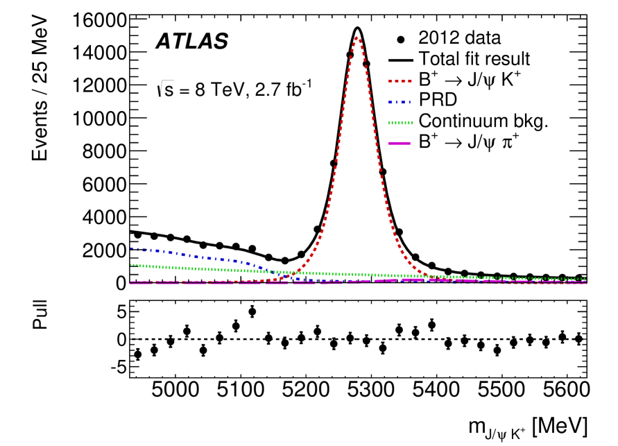
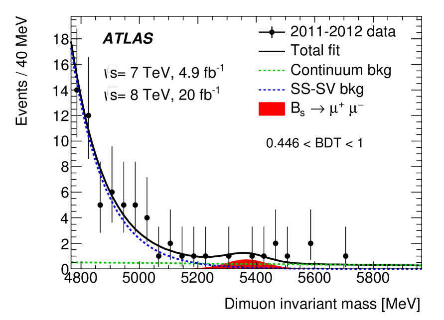
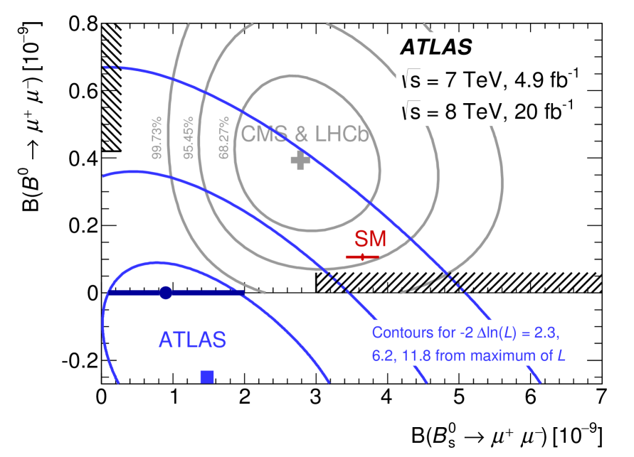
Figure 2: Left: $J/\psi K^{+}$ invariant mass distribution for $B^{+}$ candidates in the main trigger category in 2012 data. The result of the fit is overlaid. Centre: di-muon invariant mass distribution in Run 1 data, in the third continuum-BDT interval. The result of the fit for non-negative signal contributions is overlaid. Right: contours in the $\mbox{\rm BR}(B^{0}_{s}\to\mu^{+}\mu^{-}),\mbox{\rm BR}(B^{0}\to\mu^{+}\mu^{-})$ plane for intervals of $-2\,\Delta\ln(L)$ equal to $2.3$, $6.2$ and $11.8$ relative to the absolute maximum of the likelihood, without the constraint of non-negative branching fractions. The hatched areas on the axes correspond to the excluded values from the upper limits at 95% CL. Also shown are the contours for the combined CMS-LHCb result, the SM prediction, and the maximum of the likelihood with non-negative branching fractions [1].

Both $B^{+}\to J/\psi\,K^{+}$ and $B^{0}\!{}_{(s)}\to\mu^{+}\mu^{-}$ channels are measured in the fiducial volume of the $B$ meson defined as $p_{\text{T}}^{B}>8.0$ GeV and $\left|\eta_{B}\right|<2.5$. The total efficiencies within the fiducial volume include acceptance and trigger, reconstruction and selection efficiencies. All efficiency terms are computed on data-corrected MC samples separately for the three trigger selections used in 2012 and for the 2011 sample. The ratios of efficiencies enters in Eq. (2): their statistical uncertainties come from the finite size of the MC samples. The systematic uncertainties come from data corrections, trigger efficiencies, the data–MC differences, and the differences between the $B^{0}_{s}\to\mu^{+}\mu^{-}$ and the $B^{+}\to J/\psi\,K^{+}$ channels. The total uncertainty on $\mathcal{D}_{\mathrm{norm}}$ is $\pm 5.9$%. A correction to the efficiency for $B^{0}_{s}\to\mu^{+}\mu^{-}$ is needed because of the width difference $\Delta\Gamma_{s}$ between the $B^{0}_{s}$ eigenstates: the variation in the $B^{0}_{s}\to\mu^{+}\mu^{-}$ mean lifetime changes the $B^{0}_{s}$ efficiency by $+4$%.

The total yields of $B^{0}_{s}\to\mu^{+}\mu^{-}$ and $B^{0}\to\mu^{+}\mu^{-}$ events are obtained from an unbinned extended maximum-likelihood fit on the di-muon invariant mass distribution performed simultaneously across three continuum-BDT intervals. Each interval corresponds to an equal efficiency of $18\%$ for signal events, and it is ordered according to increasing signal-to-background ratio. The central plot of Figure 2 shows the di-muon invariant mass distributions in the Run 1 data in the third interval. The values determined by the fit are $N_{s}=16\pm 12$ and $N_{d}=-11\pm 9$. The systematic uncertainties related to the continuum-BDT intervals and to the the fit models are included in the likelihood with Gaussian multiplicative factors with width equal to the systematic uncertainty value. The primary result of this analysis is obtained by applying the natural boundary of non-negative yields, for which the fit returns the values $N_{s}=11$ and $N_{d}=0$.

The branching fractions for the decays $B^{0}_{s}\to\mu^{+}\mu^{-}$ and $B^{0}\to\mu^{+}\mu^{-}$ are extracted using a profile-likelihood fit. The likelihood is obtained from the one used for the yields replacing the fit parameters with the corresponding branching fractions divided by normalisation terms in Eq. (1), and including Gaussian multiplicative factors for the normalisation uncertainties. A Neyman construction [6] is used to determine the $68.3\%$ confidence interval for BR($B^{0}_{s}\to\mu^{+}\mu^{-}$) with pseudo-MC experiments, obtaining:

$$\mbox{\rm BR}(B^{0}_{s}\to\mu^{+}\mu^{-})=\left(0.9^{+1.1}_{-0.8}\right)\times 10^{-9}\,,$$ (3)

where the uncertainties are both statistical and systematic. The statistical uncertainty is dominant, with the systematic uncertainty equal to $\pm\,0.3\times 10^{-9}$. The observed significance of the $B^{0}_{s}\to\mu^{+}\mu^{-}$ signal from pseudo-MC experiments is equal to 1.4 standard deviations ($\sigma$). The expected significance for the SM prediction [3] is $3.1\sigma$. Pseudo-MC experiments are used to evaluate the compatibility with the SM prediction: for the simultaneous fit to BR($B^{0}_{s}\to\mu^{+}\mu^{-}$) and BR($B^{0}\to\mu^{+}\mu^{-}$), the result is $p=0.048\pm 0.002$, corresponding to $2.0\sigma$. The right plot in Figure 2 shows the contours in the plane of BR($B^{0}_{s}\to\mu^{+}\mu^{-}$) and BR($B^{0}\to\mu^{+}\mu^{-}$) for values of $-2\,\Delta\ln(L)$ equal to $2.3$, $6.2$ and $11.8$, relative to the maximum of the likelihood, allowing negative values of the branching fractions. The maximum within the physical boundary is shown with error bars corresponding to the $68.3$% interval for BR($B^{0}_{s}\to\mu^{+}\mu^{-}$). With the CL_s method [7], upper limits are placed on both the $B^{0}_{s}\to\mu^{+}\mu^{-}$ and $B^{0}\to\mu^{+}\mu^{-}$ branching fractions at the $95\%$ confidence level: $\mbox{\rm BR}(B^{0}_{s}\to\mu^{+}\mu^{-})<3.0\times 10^{-9}$ and $\mbox{\rm BR}(B^{0}\to\mu^{+}\mu^{-})<4.2\times 10^{-10}$. The expected significance for BR($B^{0}\to\mu^{+}\mu^{-}$) SM prediction is equal to $0.2\sigma$.

3 Angular analysis of $B^{0}\to K^{*}\mu^{+}\mu^{-}$ decays

We present here the results of the angular analysis of the decay $B^{0}\to K^{*}\mu^{+}\mu^{-}$ with the ATLAS detector, using 20.3 $\mathrm{fb}^{-1}$ of $pp$ collision data at a centre of mass energy $\sqrt{s}=8$ TeV delivered by the LHC during 2012 [8]. In order to compare with other experiments and phenomenology studies, results are presented in six different bins of $q^{2}$ in the range $0.04$ to $6.0$ $\mathrm{GeV}^{2}$, where three of these bins overlap.

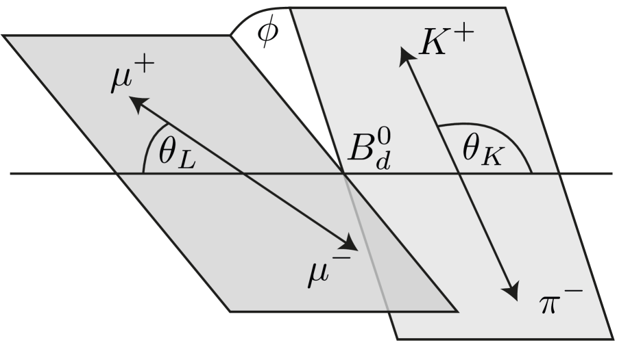
Three angular variables are used to describe the decay: the angle between the $K^{+}$ and the direction opposite to the $B^{0}$ in the $K^{*}$ centre of mass frame ($\theta_{{K}}$); the angle between the $\mu^{+}$ and the direction opposite to the $B^{0}$ in the di-muon centre of mass frame ($\theta_{{L}}$); and the angle between the two decay planes formed by the $K\pi$ and the di-muon systems in the $B^{0}$ rest frame ($\phi$). Figure 3 illustrates the angles used. The angular differential decay rate for $B^{0}\to K^{*}\mu^{+}\mu^{-}$ is a function of $q^{2}$, $\cos\theta_{{K}}$, $\cos\theta_{{L}}$ and $\phi$ is expressed as a function of the angular parameters via coefficients that may be represented by the helicity or transversity amplitudes and is written as:
$\displaystyle\!\frac{1}{\mathrm{d}\Gamma/\mathrm{d}q^{2}}\frac{\mathrm{d}^{4}\Gamma}{\mathrm{d}\cos\theta_{{L}}\mathrm{d}\cos\theta_{{K}}\mathrm{d}\phi\mathrm{d}q^{2}}=$ $\displaystyle\;\;\;\;\;\;=\frac{9}{32\pi}\Bigg{[}\frac{3(1-F_{L})}{4}\sin^{2}\theta_{{K}}$ $\displaystyle\;\;\;\;\;\;+F_{L}\cos^{2}\theta_{{K}}+\frac{1-F_{L}}{4}\sin^{2}\theta_{{K}}\cos 2\theta_{L}$ $\displaystyle\;\;\;\;\;\;-F_{L}\cos^{2}\theta_{{K}}\cos 2\theta_{L}+S_{3}\sin^{2}\theta_{{K}}\sin^{2}\theta_{{L}}\cos 2\phi$ $\displaystyle\;\;\;\;\;\;+S_{4}\sin 2\theta_{K}\sin 2\theta_{L}\cos\phi+S_{5}\sin 2\theta_{K}\sin\theta_{{L}}\cos\phi$ $\displaystyle\;\;\;\;\;\;+S_{6}\sin^{2}\theta_{{K}}\cos\theta_{{L}}+S_{7}\sin 2\theta_{K}\sin\theta_{{L}}\sin\phi$ $\displaystyle\;\;\;\;\;\;+S_{8}\sin 2\theta_{K}\sin 2\theta_{L}\sin\phi+S_{9}\sin^{2}\theta_{{K}}\sin^{2}\theta_{{L}}\sin 2\phi\Bigg{]}.$ (4)               Figure 3: Illustration of the $B^{0}\to K^{*}\mu^{+}\mu^{-}$ decay showing the angles $\theta_{K}$, $\theta_{L}$ and $\phi$ defined in the text. Angles are computed in the rest frame of the $K^{*}$, di-muon system and $B^{0}$ meson, respectively [8].
Here $F_{L}$ is the fraction of longitudinally polarised $K^{*}$s and the $S_{i}$ are angular coefficients. These angular parameters are functions of the real and imaginary parts of the transversity amplitudes of $B^{0}$ decays to $K^{*}\mu^{+}\mu^{-}$. The forward-backward asymmetry is given by $A_{\mathrm{FB}}=3S_{6}/4$. The $S_{i}$ parameters depend on hadronic form factors which have significant uncertainties at leading order. It is possible to reduce the theoretical uncertainty on the parameters extracted from data by transforming the $S_{i}$ using ratios constructed to cancel form factor uncertainties at leading order. These ratios are given by Refs [9, *Descotes-Genon:2013vna] as

$$P_{1}=\frac{2S_{3}}{1-F_{L}}\;\;\;\;\;\;\;\;P_{2}=\frac{2}{3}\frac{A_{\mathrm{FB}}}{1-F_{L}}\;\;\;\;\;\;\;\;P_{3}=-\frac{S_{9}}{1-F_{L}}\;\;\;\;\;\;\;\;P_{j=4,5,6,8}^{\prime}=\frac{S_{i=4,5,7,8}}{\sqrt{F_{L}(1-F_{L})}}.$$ (5)

All of the parameters introduced, $F_{L}$, $S_{i}$ and $P^{(\prime)}_{j}$, vary with $q^{2}$ and the data are analysed in $q^{2}$ bins to obtain an average value for a given parameter in that bin. Measurements of these quantities can be used as inputs to global fits used to determine the values of Wilson coefficients and search for new physics.

As the ATLAS detector does not have a dedicated charged-particle identification system, $K^{*}$ candidates are reconstructed to satisfy both possible $K\pi$ mass hypotheses. The invariant $K\pi$ mass is required to lie in the range $[846,946]$ MeV. The charge of the kaon candidate is used to assign the flavor of the $B$ candidate. This procedure results in an incorrect flavor tag (mistag $\omega$) of $\omega=0.1088\pm 0.0005$ ($\overline{\omega}=0.1086\pm 0.0005$).

The region $q^{2}\in[0.98,1.1]$ $\mathrm{GeV}^{2}$ is vetoed to remove any contamination from the $\phi(1020)$ resonance. The remaining data with $q^{2}\in[0.04,6.0]$ $\mathrm{GeV}^{2}$ are analysed. Two $K^{*}c\overline{c}$ control sample regions are defined for $B$ decays to $K^{*}J/\psi$ and $K^{*}\psi(2S)$, respectively as $q^{2}\in[8,11]$ and $[12,15]$ $\mathrm{GeV}^{2}$. The control samples are used to extract nuisance parameters of the signal probability density function (p.d.f.) from data. For $q^{2}$ $<6$ $\mathrm{GeV}^{2}$ the selected data sample consists of $787$ events and is composed of signal $B^{0}_{d}\to K^{*}\mu^{+}\mu^{-}$ decay events as well as background that is dominated by a combinatorial component that does not peak in $m_{K\pi\mu\mu}$ and does not exhibit a resonant structure in $q^{2}$. Above $6$ $\mathrm{GeV}^{2}$ several backgrounds pass the selection imposed, including events coming from the low mass tail of $B\to K^{*}J/\psi$. The data are analysed in the $q^{2}$ bins $[0.04,2.0]$, $[2.0,4.0]$, $[4.0,6.0]$, $[0.04,4.0]$, $[1.1,6.0]$, $[0.04,6.0]$ $\mathrm{GeV}^{2}$, where the bin width is chosen to provide a sample of signal events sufficient to perform an angular analysis and to be larger than the mass resolution.

Extended unbinned maximum likelihood fits of the angular distributions of the decay are performed on the data for each $q^{2}$ bin. The variables used in the fit are $m_{K\pi\mu\mu}$, the cosines of the helicity angles ($\cos\theta_{{K}}$ and $\cos\theta_{{L}}$), and $\phi$. The full angular distribution cannot be reliably fit given the current statistics: trigonometric transformations are used to simplify the distribution through ‘folding schemes’. Each transformation simplifies Eq. (4) such that only three parameters are extracted from each fit: $F_{L}$, $S_{3}$ and one of the other $S_{i}$ parameters. The values and uncertainties of $F_{L}$ and $S_{3}$ obtained from the four fits are consistent with each other and the results reported are those found to have the smallest systematic uncertainty. This procedure implies that $S_{6}$ ($A_{\mathrm{FB}}$) and $S_{9}$ cannot be extracted. The angular parameters of interest for these schemes are $(F_{L},S_{3},S_{i})$ where $i=4,5,6,8$. These translate into $(F_{L},P_{1},P^{\prime}_{j})$, where $j=4,5,7,8$.

$q^{2}$ [$\mathrm{GeV}^{2}$]	$n_{\mathrm{signal}}$	$n_{\mathrm{background}}$
$[0.04,2.0]$	$128\pm 22$	$122\pm 22$
$[2.0,4.0]$	$106\pm 23$	$113\pm 23$
$[4.0,6.0]$	$114\pm 24$	$204\pm 26$

$q^{2}$ [$\mathrm{GeV}^{2}$]	$n_{\mathrm{signal}}$	$n_{\mathrm{background}}$
$[0.04,4.0]$	$236\pm 31$	$233\pm 32$
$[1.1,6.0]$	$275\pm 35$	$363\pm 36$
$[0.04,6.0]$	$342\pm 39$	$445\pm 40$

Table 1: The values of fitted signal, $n_{\mathrm{signal}}$, and background, $n_{\mathrm{background}}$, yields obtained for different bins in $q^{2}$. The uncertainties indicated are statistical only [8].

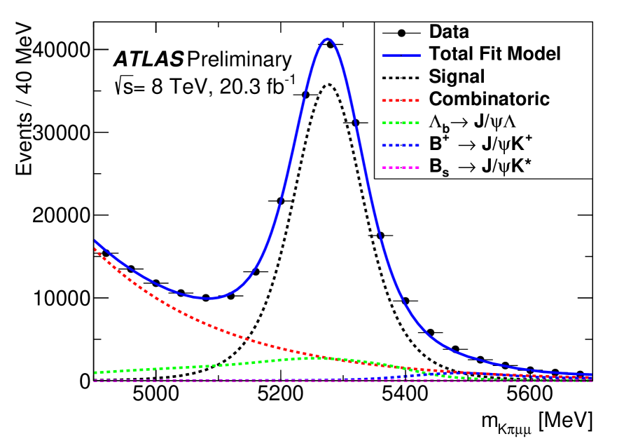
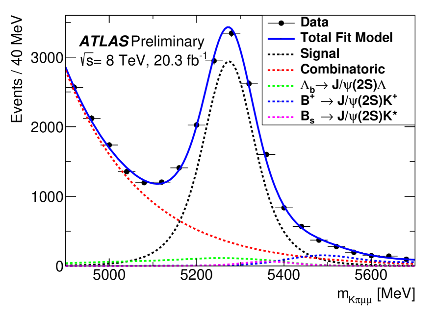
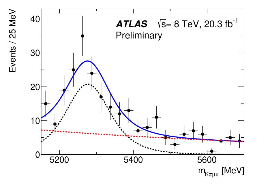
Figure 4: Control sample fits to the $K\pi\mu\mu$ invariant mass distributions for the (left) $K^{*}J/\psi$ and (centre) $K^{*}\psi(2S)$ regions. The data are shown as points and the total fit model as the solid lines. The dashed lines represent (black) signal, (red) combinatorial background, (green) $\Lambda_{b}$ background, (blue) $B^{+}$ background and (magenta) $B_{s}^{0}$ background. Right: distribution of $m_{K\pi\mu\mu}$ obtained for $q^{2}\in[0.04,2.0]$ $\mathrm{GeV}^{2}$. The (blue) solid line is a projection of the total p.d.f., the (red) dashed line represents the background, and the (black) dashed line represents the signal component. These plots are obtained from a fit using the $S_{5}$ folding scheme [8].

A two-step fit process is performed for the different signal regions in $q^{2}$. The first step is a fit to the $K\pi\mu^{+}\mu^{-}$ invariant mass distribution, using the event-by-event uncertainty on the reconstructed mass as a conditional variable. For this fit the signal shape parameters are fixed to the values obtained from fits to data control samples. The results of the fits are shown in Figures 4 and the signal yields are given in Tables 1. A second step adds the (transformed) $\cos\theta_{{K}}$, $\cos\theta_{{L}}$ and $\phi$ variables to the likelihood to extract $F_{L}$ and the $S_{i}$ parameters along with the combinatorial background shapes. Mass shape parameters and yields are fixed to the results obtained from the first step. From signal MC samples, the acceptance function is obtained as the deviation from the generated distribution of $\cos\theta_{{K}}$, $\cos\theta_{{L}}$, $\phi$ as a result of triggering, reconstruction and selection of events. The acceptance function multiplies the angular distribution in the fit. Figures 5 show for the different $q^{2}$ bins the distributions of the variables used in the fit for the $S_{5}$ folding scheme. Similar sets of distributions are obtained for the three other folding schemes: $S_{4}$, $S_{7}$ and $S_{8}$. The results of the angular fits to the data in terms of the $S_{i}$ and $P_{i}^{(\prime)}$ can be found in Table 2.

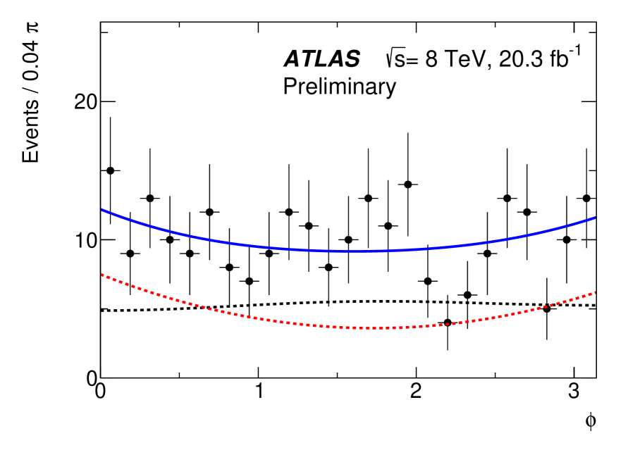
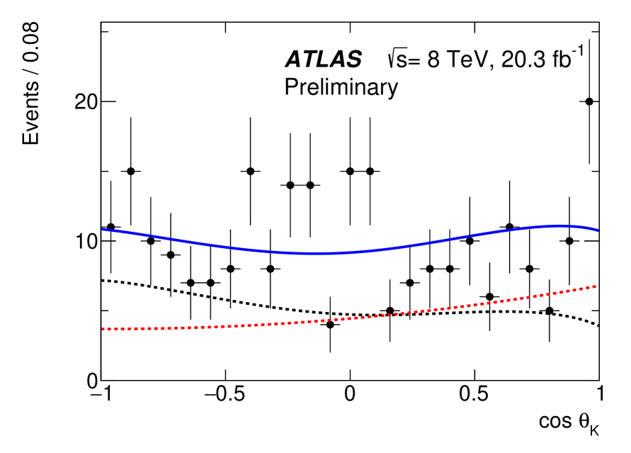
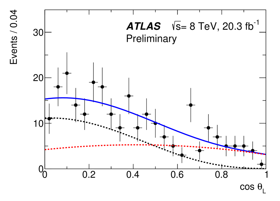
Figure 5: The distributions of (left) $\phi$, (centre) $\cos\theta_{{K}}$, and (right) $\cos\theta_{{L}}$ obtained for $q^{2}\in[0.04,2.0]$ $\mathrm{GeV}^{2}$. The (blue) solid line is a projection of the total p.d.f., the (red) dashed line represents the background, and the (black) dashed line represents the signal component. These plots are obtained from a fit using the $S_{5}$ folding scheme [8].

$q^{2}$ [$\mathrm{GeV}^{2}$]	$P_{1}$	$P_{4}^{\prime}$	$P_{5}^{\prime}$	$P_{6}^{\prime}$	$P_{8}^{\prime}$
$[0.04,2.0]$	$-0.06\pm 0.30\pm 0.10$	$0.39\pm 0.51\pm 0.25$	$0.67\pm 0.26\pm 0.16$	$-0.18\pm 0.21\pm 0.04$	$-0.22\pm 0.38\pm 0.14$
$[2.0,4.0]$	$-0.78\pm 0.51\pm 0.42$	$-0.96\pm 0.39\pm 0.26$	$-0.33\pm 0.31\pm 0.13$	$0.31\pm 0.28\pm 0.19$	$0.84\pm 0.32\pm 0.31$
$[4.0,6.0]$	$0.00\pm 0.47\pm 0.26$	$0.81\pm 0.42\pm 0.24$	$0.26\pm 0.35\pm 0.17$	$0.06\pm 0.27\pm 0.13$	$-0.19\pm 0.33\pm 0.07$
$[0.04,4.0]$	$-0.22\pm 0.26\pm 0.16$	$-0.38\pm 0.31\pm 0.22$	$0.32\pm 0.21\pm 0.10$	$0.01\pm 0.17\pm 0.10$	$0.30\pm 0.26\pm 0.19$
$[1.1,6.0]$	$-0.17\pm 0.31\pm 0.14$	$0.07\pm 0.28\pm 0.18$	$0.01\pm 0.21\pm 0.07$	$0.03\pm 0.17\pm 0.11$	$0.18\pm 0.22\pm 0.16$
$[0.04,6.0]$	$-0.15\pm 0.23\pm 0.10$	$0.07\pm 0.26\pm 0.18$	$0.27\pm 0.19\pm 0.07$	$0.03\pm 0.15\pm 0.10$	$0.11\pm 0.21\pm 0.14$

Table 2: The values $P_{1}$, $P_{4}^{\prime}$, $P_{5}^{\prime}$, $P_{6}^{\prime}$ and $P_{8}^{\prime}$ obtained for different bins in $q^{2}$. The uncertainties indicated are statistical and systematic, respectively [8].

A total of seven inclusive and eleven exclusive $B^{0}$, $B^{0}_{s}$, $B^{+}$ and $\Lambda_{b}$ background samples are studied as systematic uncertainties. Two additional background contributions are observed in the $\cos\theta_{{K}}$ and $\cos\theta_{{L}}$ distributions. They are also treated as systematic effects given the current statistics. A peak in $\cos\theta_{{K}}$ is found at about 1.0 and appears to come from two contributions. One arises from $B^{+}$ decays, such as $B^{+}\to K^{+}\mu\mu$ and $B^{+}\to\pi^{+}\mu\mu$, where an extra track is combined with the hadron to form a fake $K^{*}$. A veto on events with a three-track invariant mass within a 50 MeV mass window around the nominal $B^{+}$ mass reduces the size of the peak in $\cos\theta_{{K}}$. The second contribution comes from two charged tracks forming a fake $K^{*}$ candidate and it is observed in the $K\pi$ sidebands away from the $K^{*}$ meson. The origin of this source of background is not fully understood. The background that peaks in $\cos\theta_{{L}}$ is studied using Monte Carlo simulated events for the decays $D^{0}\to K\pi$, $D^{+}\to K\pi\pi$, $D^{+}_{s}\to KK\pi$, and $D^{*+}_{s}\to KK\pi$. Events with an intermediate charm meson, $D^{0}$, $D^{\pm}_{(s)}$ and $D^{*+}_{s}$ are found to accumulate around 0.7 in $|\cos\theta_{{L}}|$. A 30 MeV wide veto window about the reconstructed charm meson mass can be applied to eliminate this background.

The main systematic uncertainties come from backgrounds, mainly the fake $K^{*}$ background and the background arising from partially reconstructed $B\to D^{0}/D^{+}/D^{+}_{s}/D^{*}_{s}X$ decays. Other systematic uncertainties in decreasing order of importance are coming from the background p.d.f. shape, the acceptance function, the combinatorial background, tracking alignment, knowledge of the magnetic field, bias from the maximum likelihood estimator, $p_{\text{T}}$ spectrum of $B$ candidates, and scalar contributions from non-resonant $K\pi$ transitions, The total systematic uncertainties for the $P_{i}^{(\prime)}$ parameters fitted are presented in Table 2.

The results of theoretical approaches of Ciuchini et al. (CFFMPSV) [11], Descotes-Genon et al. (DHMV) [12], and Jäger and Camalich (JC) [13, 14] are shown in Figure 6 for the $P^{(\prime)}$ parameters. With the exception of the $P_{4}^{\prime}$ and $P_{5}^{\prime}$ measurements in $q^{2}\in[4.0,6.0]$ $\mathrm{GeV}^{2}$ and $P_{8}^{\prime}$ in $q^{2}\in[2.0,4.0]$ $\mathrm{GeV}^{2}$ there is good agreement between theory and measurement. The deviation observed for $P_{4}^{\prime}$ ($P_{5}^{\prime}$) is consistent with the one reported by the LHCb Collaboration [15], and it is approximately 2.5 (2.7) standard deviations away from the calculation of DHMV. The deviations are less significant for the other theoretical approaches. All measurements are found to be within three standard deviations of the range covered by the different predictions. Hence, including experimental and theoretical uncertainties, the measurements presented here are found to be in accordance with the expectations of the SM contributions to this decay.

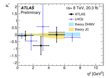
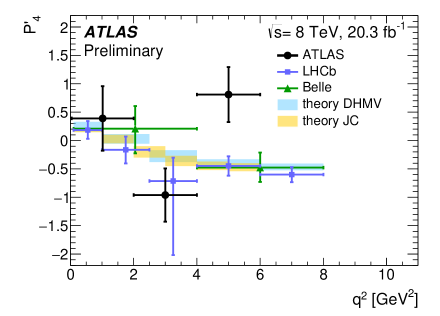
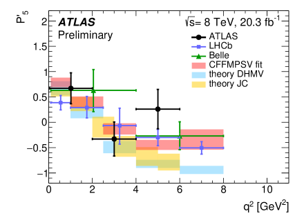
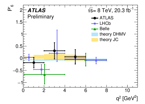
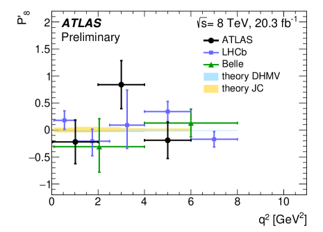
Figure 6: The measured values of $P_{1}$, $P_{4}^{\prime}$, $P_{5}^{\prime}$, $P_{6}^{\prime}$, $P_{8}^{\prime}$ compared with predictions from the theoretical calculations discussed in the text. Statistical and total uncertainties are shown for the data, i.e. the inner mark indicates the statistical uncertainty and the total error bar the total uncertainty [8].

References

- [1] ATLAS Collaboration, Study of the rare decays of and into muon pairs from data collected during the LHC Run 1 with the ATLAS detector, Eur. Phys. J. C 76 (2016) 513, [1604.04263]
- [2] ATLAS Collaboration, The ATLAS Experiment at the CERN Large Hadron Collider, JINST 3 (2008) S08003
- [3] C. Bobeth, M. Gorbahn, T. Hermann, M. Misiak, E. Stamou et al., in the standard model with reduced theoretical uncertainty, Phys. Rev. Lett. 112 (2014) 101801, [1311.0903]
- [4] LHCb Collaboration, R. Aaij et al., Measurement of the branching fraction and effective lifetime and search for decays, Phys. Rev. Lett. 118 (2017) 191801, [1703.05747]
- [5] CMS and LHCb Collaborations, Observation of the rare decay from the combined analysis of CMS and LHCb data, Nature 522 (2015) 68, [1411.4413]
- [6] J. Neyman, “Outline of a theory of statistical estimation based on the classical theory of probability.” Phil. Trans. R. Soc. London A, 236 (1937) 333-380
- [7] A. L. Read, Presentation of search results: The technique, J. Phys. G 28 (2002) 2693–2704
- [8] ATLAS Collaboration, “Angular analysis of decays in collisions at with the ATLAS detector.” ATLAS-CONF-2017-023, 2017
- [9] S. Descotes-Genon, J. Matias, M. Ramon and J. Virto, Implications from clean observables for the binned analysis of at large recoil, JHEP 01 (2013) 048, [1207.2753]
- [10] S. Descotes-Genon, T. Hurth, J. Matias and J. Virto, Optimizing the basis of observables in the full kinematic range, JHEP 05 (2013) 137, [1303.5794]
- [11] M. Ciuchini, M. Fedele, E. Franco, S. Mishima, A. Paul, L. Silvestrini et al., decays at large recoil in the Standard Model: a theoretical reappraisal, JHEP 06 (2016) 116, [1512.07157]
- [12] S. Descotes-Genon, L. Hofer, J. Matias and J. Virto, On the impact of power corrections in the prediction of observables, JHEP 12 (2014) 125, [1407.8526]
- [13] S. Jäger and J. Martin Camalich, On at small dilepton invariant mass, power corrections, and new physics, JHEP 05 (2013) 043, [1212.2263]
- [14] S. Jäger and J. Martin Camalich, Reassessing the discovery potential of the decays in the large-recoil region: SM challenges and BSM opportunities, Phys. Rev. D 93 (2016) 014028, [1412.3183]
- [15] LHCb Collaboration, R. Aaij et al., Angular analysis of the decay using 3 fb-1 of integrated luminosity, JHEP 02 (2016) 104, [1512.04442]