Probing features in the primordial perturbation spectrum with large-scale structure data

Abstract

The form of the primordial power spectrum (PPS) of cosmological scalar (matter density) perturbations is not yet constrained satisfactorily in spite of the tremendous amount of information from the Cosmic Microwave Background (CMB) data. While a smooth power-law-like form of the PPS is consistent with the CMB data, some PPS with small non-smooth features at large scales can also fit the CMB temperature and polarization data with similar statistical evidence. Future CMB surveys cannot help distinguish all such models due to the cosmic variance at large angular scales. In this paper, we study how well we can differentiate between such featured forms of the PPS not otherwise distinguishable using CMB data. We ran 15 $N$-body DESI-like simulations of these models to explore this approach. Showing that statistics such as the halo mass function and the two-point correlation function are not able to distinguish these models in a DESI-like survey, we advocate to avoid reducing the dimensionality of the problem by demonstrating that the use of a simple three-dimensional count-in-cell density field can be much more effective for the purpose of model distinction.

1 Introduction

So far, the CMB data have been able to provide us with the most valuable information about the early Universe (EU). CMB temperature anisotropy and E-mode polarization data contain a convolved form of the primordial power spectrum (PPS) of scalar (matter density) perturbations and of the evolution of these primordial fluctuations through different epochs of the Universe.

To better understand the physics of the EU, it is extremely important to put constraints on the shape of the PPS with high precision. In particular, looking for small features in the PPS is very important to evaluate whether it is necessary to go beyond the simplest theoretical models of the EU. For instance, in inflationary cosmology the Universe underwent a phase of rapid expansion known as inflation in the remote past, seeding structure formation. In its simplest form, inflation yields a power-law-like, close to scale-invariant PPS

$$P_{i}(k)=A_{s}\left(\frac{k}{k_{0}}\right)^{n_{s}-1},$$ (1)

where the spectral index $n_{s}$ is close to unity and weakly depends on the inverse scale $k$, so it can be approximated by a constant value $n_{s}\simeq 0.96$ over the measured range of scales ($\sim 1-10^{4}$ Mpc) (Starobinsky, 1980; Guth, 1981; Mukhanov & Chibisov, 1981; Linde, 1982). Thus, the observed PPS is very well described by only two phenomenological dimensionless constants.

However, it is clear that this is the first approximation only, and at a higher level of accuracy $\lesssim 10\%$, one can well expect the existence of small non-smooth features in the PPS whose quantitative description would require more phenomenological parameters (at least two of them – their location and relative magnitude). From the theoretical point of view, some new physics will be needed for their explanation and derivation. It should be noted that this is not specific for inflationary cosmology only, but equally well refers to any viable alternative cosmology of the EU. It is simply that an alternative cosmology will require different additional physics to predict the same observed feature in the PPS, if it can accomplish it at all.

In this work we mainly focus on few different inflationary models that can generate extra features to the power-law shape of the PPS and compare them with the case of a power-law-like form of the PPS predicted by the simplest inflationary models with one, maximum two, free dimensionless parameters fixed by observations. However, as we mentioned earlier, the whole analysis is mainly about detecting small non-smooth features in the PPS, and thus it can be relevant for any alternative EU scenario.

The study of the cosmological microwave background (CMB), has put strong constrains on power-law-like form of the PPS predicted by simple single-field slow-roll inflationary models (e.g. Planck Collaboration XX, 2016). However, degeneracies in the CMB data allow also several other models to survive where these models can generate some prominent features in the form of the PPS (e.g. Starobinsky, 1992; Adams et al., 2001; Joy et al., 2008; Joy et al., 2009; Hazra et al., 2014a, b; Horiguchi et al., 2017; Hazra et al., 2018). It is thus important to falsify these models and test how well we can distinguish between them using different cosmological observations.

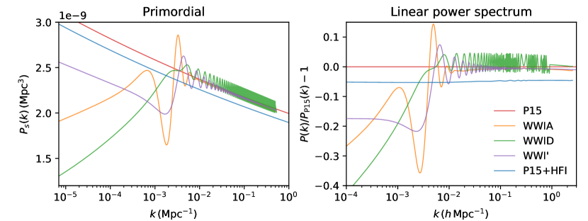
Figure 1: Left: PPS of our five models. Bottom: linear matter power spectra normalized by the reference (P15) case.

In this work, we aim to assess the ability of the large-scale structure (LSS) to differentiate between few forms of the PPS, result from some inflationary models, that are indistinguishable from each other using the CMB data alone. Indeed, observationally, one has two main anchors that the cosmology must fit. At high redshift, the CMB has revealed a tremendous amount of information, strengthening the concordance model of cosmology and rising cosmology to a precision science. However, even though polarization still holds valuable information, we are about to reach the limits of what can be learned by the temperature anisotropy on large scales due to cosmic variance. At low redshift, the large-scale structure (LSS) of the Universe, thanks to their three-dimensional structure, also carries a large amount of information. Any viable model must therefore confront these two anchors and fit all the data appropriately.

Upcoming surveys such as the dark energy spectroscopic instrument (DESI Collaboration et al., 2016a), EUCLID (Laureijs et al., 2011), or LSST (Ivezic et al., 2008) will probe the Universe to an unprecedented scale and it is important to know how well we can use them to learn more about the physics of the early universe. Cosmological simulations have now been extensively used to understand non-linear structure formation (e.g. Springel et al., 2005) and test dark energy (Alimi et al., 2012; Baldi, 2012), modified gravity (Zhao et al., 2011; Brax et al., 2012, 2013; Llinares & Mota, 2014; L’Huillier et al., 2017), neutrinos (Baldi et al., 2014), and warm dark matter (Hellwing et al., 2016). In this work, we use cosmological $N$-body simulations, similar to what we expect to observe from DESI, with some specific forms of the PPS and study how well we can distinguish between these models.

Section 2 presents the models and the simulations, the results are shown in § 3, and we draw our conclusions in § 4.

Table 1: Cosmological parameters of models. The last column shows the improvement in $\chi^{2}$ of the WWI models with respect to the reference P15 case. Note that, since P15+HFI uses a different data set, we do not compare its $\chi^{2}$.

Model	$\Omega_{\text{m}}$	$H_{0}$	$\sigma_{8}$	$n_{\mathrm{s}}$	$\Delta\chi^{2}$
		($\mathrm{k}\mathrm{m}\,\mathrm{s}^{-1}$
		$\,\mathrm{M}\mathrm{p}\mathrm{c}^{-1}$)
P15	0.317	67.05	0.836	0.9625	0
WWIA	0.320	66.86	0.834	-	7
WWID	0.318	67.01	0.842	-	13.3
WWI′	0.317	67.04	0.834	-	12
P15+HFI	0.319	66.93	0.816	0.9619	-

2 Models and simulations

2.1 The models

In this section, we present the different early Universe models studied in this work. The choice of these models is solely due to the form of the primordial spectrum they generate and the fact that they all can fit the Planck CMB data very well. Due to the excellent accuracy with which the standard $\Lambda$CDM 6-parameter model fits the Planck data with $l>40$, we restrict ourselves to models which, first, produce localised features in the PPS and, second, fit the smooth small-scale part of the PPS outside the features as well as possible in terms of the PPS slope $n_{s}\approx 0.965$ measured by Planck. Characteristic examples of such models are the Wiggly-wipped inflationary (WWI) models introduced in Hazra et al. (2014a, 2016). These models produce a better fit to the CMB data than the power-law model, and are thus not currently distinguishable from each other using the CMB data alone. Our reference model is the Planck Collaboration XIII (2016) best-fitting power-law (TTTEEEE+lowTEB+BKP) cosmology (P15). We used three different Wiggly-whipped inflation models (WWI, Hazra et al., 2014a, 2016), namely WWIA, WWID, and WWI^′. Note that the constraints on the WWI models used here are based on the Planck 2015 results (Hazra et al., 2016). Finally, in order to study the effects of a change of cosmology within the power-law paradigm, we also include the Planck 2015 TTTEEE + lowTEB + BKP + HFI (P15+HFI) best-fitting cosmology.

WWIA and WWID provide an improvement of $7$ and $13.3$ in $\chi^{2}$ compared to P15, respectively. They are the local best fits obtained from the same potential having a discontinuity. This potential has four extra parameters compared to the standard slow roll case. WWI^′, on the other hand, provides a $\Delta\chi^{2}=12$ improvement in fit with only two extra parameters. WWI^′ has a discontinuity in the derivative of a continuous potential. For a complete table of likelihood comparison, see Hazra et al. (2016). Table 1 summarized the best-fitting cosmological parameters of each model, and the last column shows the improvement in $\chi^{2}$ of the WWI models with respect to P15. We aim to study their effects on the large-scale structure and assess the power of the LSS to constrain these models, complementary to the CMB.

We note here again that the main goal of this study is not to focus on the particular models considered here, but rather to try to separate between different featured forms of the PPS that are not distinguishable from the CMB data alone.

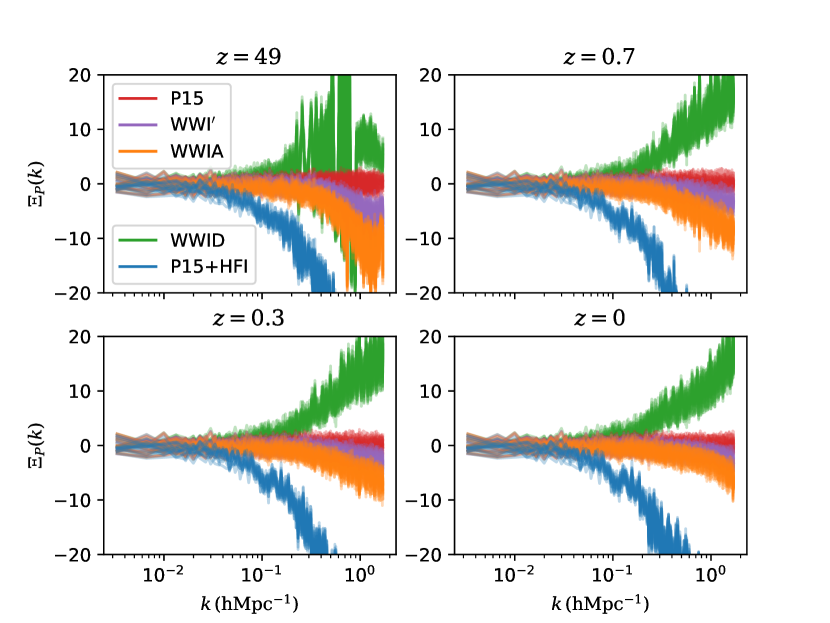
Figure 2: Normalized difference of the power spectrum of each simulation with the average over the P15 case in units of the standard deviation of the P15 case in the initial conditions (top left), and at $z=0.7$ (top right), 0.3 (bottom left), and 0 (bottom right).

The effects of the EU model translate into features in the PPS (Fig. 1), where the power spectrum of the overdensity field

$$\delta(\textbf{{x}}) =\frac{\rho(\textbf{{x}})-\bar{\rho}}{\bar{\rho}}$$ (2)

is given by

$$\left\langle\left\lvert\delta(\textbf{{k}})\delta^{*}(\textbf{{k}})\right\rvert\right\rangle_{\left\lvert\textbf{{k}}\right\rvert=k} =(2\pi)^{3}\delta^{\text{D}}{(\textbf{{k}}+\textbf{{k'}})}P(k),$$ (3)

where $\delta(\textbf{{k}})$ is the Fourier transform of $\delta(\textbf{{x}})$, and $\left\langle\cdot\right\rangle$ denotes an ensemble average. In the linear regime, the matter power spectrum can be calculated from the primordial one by a Boltzmann solver such as CAMB (Lewis et al., 2000).

The left-hand panel of Fig. 1 shows the PPS of the different models. The WWI models essentially results in a superimposition of oscillatory features on to a smooth power-law. We note that these models give indistinguishable CMB angular power spectra. The right-hand panel shows the linear matter power spectra divided by the reference P15 case.

Most of the difference between the models arises on very large scales ($k\leq${10}^{-2}$\,h\,\mathrm{Mpc}^{-1}$). On these very large-scales, due to the considered volume, the scatter is very large (few Fourier modes per bin at low-$k$), and the models cannot be distinguished with upcoming surveys. However, the WWI models also show non-power law features at intermediate scales ($10^{-2}<k<${10}^{-1}$\,h\,\mathrm{Mpc}^{-1}$). Therefore, it is necessary to go to the mildly to fully non-linear regime, hence the need for cosmological simulations.

2.2 The simulations

We used the Gadget-2 TreePM cosmological code (Springel, 2005). The simulation comprises $1024^{3}$ particles in a ${1890}\,h^{-1}\,\mathrm{Mpc}$ box, assuming a flat-$\Lambda$CDM cosmology. The choice of volume is motivated by the expected DESI volume at $z=0.9$ with a redshift depth of 0.1 (DESI Collaboration et al., 2016a, b). The cosmological parameters of each model are summarized in Table 1.

The initial conditions were generated with the second-order Lagrangian perturbation theory (2LPT) 2LPTic at redshift 49, from a Gaussian random field, since these models have very small non-gaussianities (Hazra et al., 2014a). 2LPT and high initial redshift (for the considered mean particle separation) yield an accurate power spectrum and mass function at low redshift (Scoccimarro, 1998; Crocce et al., 2006; L’Huillier et al., 2014).

The initial matter power spectra were obtained at $z=0$ by CAMB, and ($z_{i}=49$) using their own cosmology. For each model, we chose the best-fitting cosmology given by a modified version of CAMB (Hazra et al., 2014a, b).

We note that our $k$-space resolution of $k_{0}=2\pi/L=$3.3\text{\times}{10}^{-3}$\,h\,\mathrm{Mpc}^{-1}$ resolves the oscillatory features of the WWI models (the modes that are actually sampled are $k_{0}\sqrt{i^{2}+j^{2}+l^{2}},(i,j,l)\in\{0,\dots,N/2\}$).

3 Results

3.1 Power spectrum

In order to estimate the matter power spectrum (PS) in the non-linear regime, we used the ComputePk code (L’Huillier, 2014) to calculate the matter density field in a grid with $N_{\text{c}}^{3}$ cells, with $N_{\text{c}}=1024$, using the triangular shape cloud (TSC) mass assignment scheme (Hockney & Eastwood, 1988).

Fig. 2 shows at a given $k$

$$\Xi_{P_{i}}(k) =\frac{P_{i}(k)-\left\langle P_{\text{P15}}(k)\right\rangle}{\sigma_{P_{\mathrm{P15}}}(k)},$$ (4)

the deviation of the PS of simulation of each simulation $i$ with respect to the average of the PS of the P15 case $\left\langle P_{\text{P15}}(k)\right\rangle$ in units of the standard deviation $\sigma_{P_{\mathrm{P15}}}(k)$ in the initial conditions (top-left), and at redshifts 0.7 (top-right), 0.3 (bottom-left), and 0 (bottom-right). Each line shows one realization of the PPS, therefore, each model has 15 overlapping lines.

At the initial redshift (upper left), all models give different power spectra, and are visually distinguishable. On very large scales, due to the finite volume, only a few modes are sampled. Therefore, $\sigma_{P_{\mathrm{P15}}}(k)$ is large and the different simulations cannot be distinguished from each other.

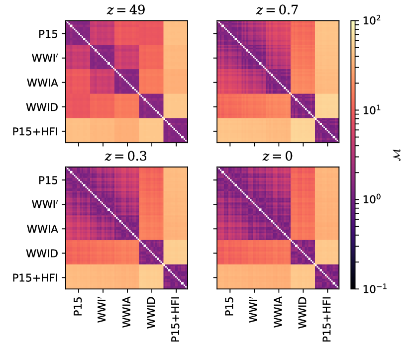
(a) Separability matrix M for the power spectrum in Fig. 2.

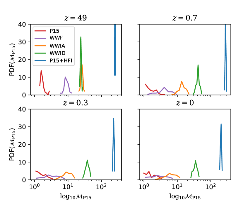
(b) Distribution of ${M}_{\mathrm{P15}_{i},\text{mod}^{n}_{j}}$.

Figure 3:

On smaller scales ($k\geq$0.2$\,h\,\mathrm{Mpc}^{-1}$), some of the oscillations in the WWID PS are still visible at redshifts of $z\simeq 0.7$). As time evolves, these oscillations are smeared out by the mode-mixing in the non-linear regime, and have essentially disappeared by redshift 0. WWID shows some excess of power, consistent with its linear PS and larger $\sigma_{8}$, and on small scales ($\geq$0.5$\,h\,\mathrm{Mpc}^{-1}$) can be distinguished from P15. However, WWIA and WWI^′ show a very similar PS to P15, and they are not distinguishable. This is consistent with their cosmological parameters which are very close to those of P15, and with the small amplitude of the oscillatory features in their linear PS.

In order to quantify the distance between any two simulations, we define the separability matrix as the root mean square of the normalized difference (with respect to P15) between the two simulations:

$${M}_{\text{mod}^{m}_{i},\text{mod}^{n}_{j}}=\sqrt{\frac{1}{N_{k}}\sum_{k}(\Xi_{P_{\text{mod}^{m}_{i}}}(k)-\Xi_{P_{\text{mod}^{n}_{j}}}(k))^{2}},$$ (5)

where mod${}^{n}_{j}$ is the $j$th simulation of model $n$. M is thus constituted of $N_{\text{models}}^{2}$ blocks of $N_{\text{real}}^{2}$, where $N_{\text{models}}=5$ and $N_{\text{real}}=15$. M is symmetric by construction, and its component are the root mean square of the deviation between two models, which becomes larger when two models are more distant. We stress that the choice of the normalization factor $\sigma_{\mathrm{P15}}$ has little impact on the results, since at a given $k$, all models have similar fluctuation. Fig. 3(a) shows the matrix M corresponding to Fig. 2. At $z=49$, it can be easily seen that the diagonal blocks have lower values: two simulations from the same model are closer to each other than two simulations from different models. Therefore, in the initial conditions, each model can be easily distinguished from the others. However, as time evolves, some models become confused with others. For instance, at $z=0$, WWI^′, WWIA, and P15 show similar values, and it is difficult to distinguish them.

The matrix M contains a huge amount of information, which can be used to distinguish between models in a quantitative way. Since our goal is primarily to distinguish featured PPS from the power-law case, we focus on the reference P15 model, and use M for this purpose. Similar procedure can be applied to any model. Fig. 3(b) shows the distribution of the values of $M_{\mathrm{P15}_{i},\text{mod}^{n}_{j}}$, for all realizations $i$ and $j$. At $z=49$, the distribution of $M_{\mathrm{P15}_{i},\text{mod}^{n}_{j}}$ does not overlap with those of $M_{\mathrm{P15}_{i},\text{mod}^{n}_{j}}$ for mod${}^{n}\neq$ P15, confirming our visual distinction between the models. At lower redshifts, the distributions start to overlap with P15: WWW^′ from $z=0.7$, and WWA from $z=0.3$, while P15+HFI and WWID stay apart. Therefore, the distributions of $M_{\mathrm{P15}_{i},\text{mod}^{n}_{j}}$ appears to be a useful metric to quantify the separability of the models. However, these results indicates that the power spectrum is not adequate to distinguish between the models considered in this work as there are overlaps between PDFs at observable redshifts.

3.2 Halo mass function

The next natural step after studying the density power spectrum is the halo mass function (Press & Schechter, 1974; Reed et al., 2007). As studied in Hazra (2013), features in the power spectrum are expected to affect the halo formation rate and the mass function. However, due to the non-linear nature of halo formation, passing from the power spectrum to the halo mass function is not trivial, hence the need for numerical simulations. We identified the haloes in the simulations with the PFOF code (Roy et al., 2014), a massively-parallel Friends-of-Friends algorithm (Davis et al., 1985). Particles closer than $b\,\bar{d}$, where $\bar{d}$ is the mean particle separation and $b$ the linking length, set to 0.2, are grouped together. We kept all haloes with number of particles $N_{\text{p}}\geq 29$, yielding a minimum mass of $$1.6\text{\times}{10}^{13}$\,h^{-1}\,M_{\odot}$, corresponding to groups and clusters of galaxies.

Fig. 4 shows the normalized difference of the mass function of simulation $i$ defined as

$$\Xi_{f_{i}}(M) =\frac{n^{\prime}_{i}(M)-\left\langle n^{\prime}_{\mathrm{P15}}(M)\right\rangle}{\sigma_{P15}(M)},$$ (6)

where

$$n^{\prime}(M) =\frac{\mathrm{d}{n}}{\mathrm{d}{M}},$$ (7)

and $n(>M)$ is the cumulative number density of haloes more massive than $M$, and $\bar{\rho}$ is the matter density.

Figure 4: Normalized difference of the halo mass function at $z=0,0.3$, and 0.7.

Due to its lack of power on small-scales, P15+HFI yields a lower mass function, up to 20% lower than P15, while WWID shows some excess, especially at the mass scale of $${10}^{15}$\,h^{-1}\,M_{\odot}$. Interestingly, WWIA can now be distinguished at $z=0$, while at higher redshift, it is closer to P15. However, given the small volume at $z=0$, obtaining an accurate mass function may be difficult. Moreover, WWI^′ is still indistinguishable from P15.

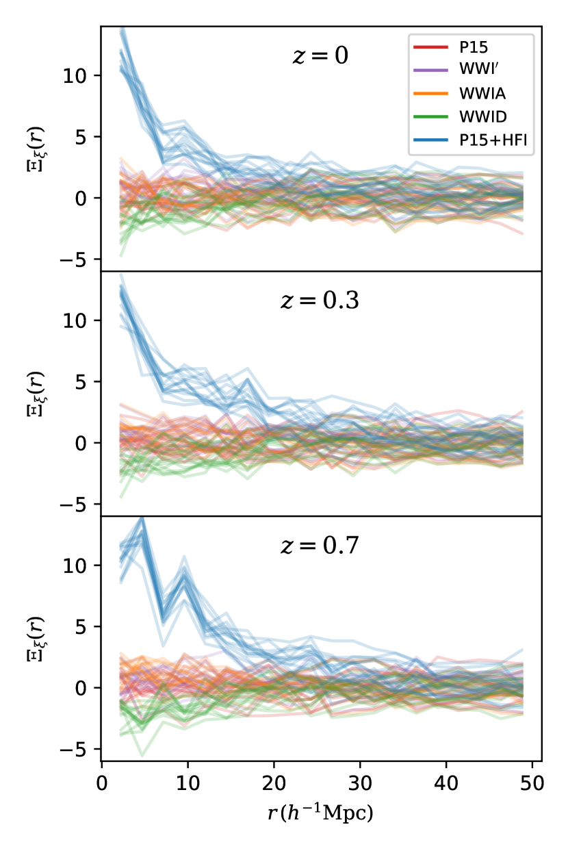
Figure 5: Normalized difference of the halo correlation function with respect to P15.

3.3 Halo two-point correlation function

Another statistics, directly comparable to observations, is the halo two-point correlation function (2pcf) $\xi$, which measures the excess of pair clustering at a distance $r$ with respect to the random case. We calculated the isotropic two-point correlation $\xi(r)$ function of FOF haloes using the kstat code. We used the Landy & Szalay (1993) estimator

$$\xi=\frac{DD-2DR+RR}{RR},$$ (8)

where DD, DR, and RR are the data-data, data-random, and random-random pair counts, respectively.

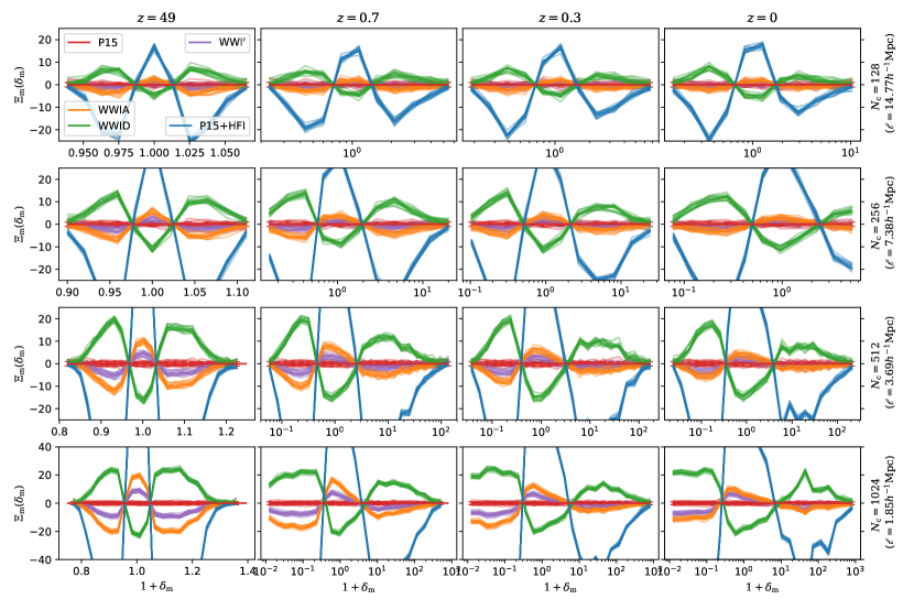
Figure 6: Normalized difference of the matter density histogram with the average of the P15 case.

Fig. 5 shows the normalized difference in the 2pcf of each simulation with respect to the P15 case, at $z=0$ (top), 0.3 (middle), and 0.7 (bottom). Only P15+HFI, and to a lesser extent, WWID, can be distinguished due to their different clustering on small scales, while on large scales, and for other models at all scales, the fluctuations are too large, making them essentially indistinguishable.

3.4 Three-dimensional count-in-cell density field

The previous sections showed the inability of statistics such as the power spectrum or the halo mass or two-point correlation function, to distinguish between WWI^′ and P15 (however, P15+HFI and WWID could be distinguished by their power spectra, and WWIA marginally with the mass function at $z=0$). Therefore, one needs to find appropriate statistics. A drawback of the matter power spectrum is that it reduces the dimensionality of the problem from three to one dimension, losing information in the process. Therefore, we looked at the three-dimensional density field.

We calculated the probability distribution function (PDF) of the dark matter density field binned in $N_{\text{c}}^{3}$ cells, with $N_{\text{c}}\in\{128,256,512,1024\}$. The density field follows a close to lognormal distribution (e.g. Shin et al., 2017). The density was calculated using ComputePk, with a TSC scheme, as in § 3.1. Fig. 6 shows the normalized difference of each simulation with respect to P15.

P15+HFI shows an excess probability at $1+\delta\approx 1$, and a lack at $1+\delta\gg 1$ and $1+\delta\ll 1$ with respect to P15, while WWID shows the opposite trend. This is consistent with the lower amplitude of the power spectrum of P15+HFI, which yields smaller fluctuations.

Since WWID and P15+HFI can be distinguished from the amplitude of their power spectrum (see § 3.1), we will focus on the remaining models, namely WWIA and WWI^′. At the coarser level ($128^{3}$, top row), even in the initial conditions, it is not easy to distinguish by eyes the distributions of the WWIA, WWI^′, and P15 cases. As the resolution of the mesh gets finer (towards lower rows), the PDFs show more and more difference. For intermediate meshes (256 and 512 cases), the PDF can be distinguished in the initial conditions and up to redshift 0.7, and for the $N_{\text{c}}=1024^{3}$ case, all models have their PDF clearly separated from the other models.

To quantify the separability of the models, we show the separability matrix M of the matter density distribution in Fig. 7. Clearly, for low-resolution cases ($N_{\text{c}}=128$ or 256), only in the initial density field we can distinguish between the models, while for high enough resolution (512 or 1024), all models can be distinguished. This is further supported by the distribution of $M_{\mathrm{P15}_{i},\text{mod}^{n}_{j}}$, the first column of the matrix, shown in Fig. 8. While for the previous estimators, the distribution of $M_{\mathrm{P15}_{i},\text{P15}_{j}}$ and $M_{\mathrm{P15}_{i},\text{WWI}^{\prime}_{j}}$ were overlapping, they are now well separated at $z=0.7$. Therefore, the three-dimensional matter density field is able to distinguish between all our models presented here, at least at $z=0.7$.

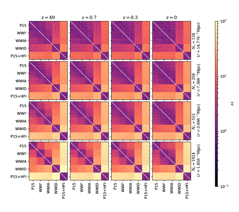
Figure 7: Separability matrix of the matter density

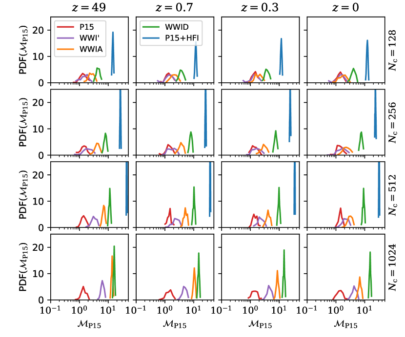
Figure 8: Distribution of $M_{\mathrm{P15}_{i},\text{mod}^{n}_{j}}$ for the matter density shown in Figs. 6 and 7.

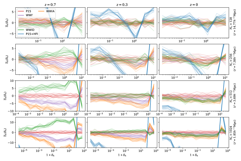
Figure 9: Normalized difference of the PDFs of the mass-weighted halo density with respect to the P15 case for $N_{\text{c}}=128$, 256, 512, and 1024 (from top to bottom).

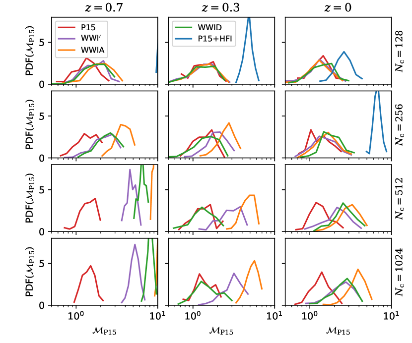
Figure 10: Distribution of $M_{\mathrm{P15}_{i},\text{mod}^{n}_{j}}$ for the halo density distribution.

The normalized difference in the matter density count-in-cell gives us important hint as to how the EU affects the LSS. However, matter is not directly observable, and we have to understand how biased tracers such as galaxies are affected. For that purpose, we applied the same technique to FoF haloes.

Fig. 9 shows the normalized difference in the PDFs of the mass-weighted halo density with respect to the average of the P15 case. The distribution of $M_{\text{P15}_{i},\text{mod}^{n}_{j}}$ is shown in Fig. 10. We used the mass-weighted rather than number-weighted halo density, since the former shows a tighter correlation with the matter density field (Jee et al., 2012; Uhlemann et al., 2018). In the $N_{\text{c}}=128$ case, the statistics are very noisy, due to the small number of pixels, which only marginally allows us to distinguish P15+HFI from the rest: all models are visually indistinguishable in Fig. 9, which is confirmed by the overlap of the distributions of $M_{\text{P15}_{i},\text{mod}^{n}_{j}}$ in Fig. 10. When going to smaller pixels, it becomes possible to distinguish between the models at $z=0.7$ for $N_{\text{c}}\geq 512$. In Fig. 10, it can clearly be seen that the distribution of $M_{\text{P15}_{i},\text{P15}_{j}}$ (red) is well separated from the other models $M_{\text{P15}_{i},\text{mod}^{n}_{j}}$.

4 Discussion and summary

In order to distinguish five different degenerate (with respect to the CMB data) forms of the PPS (Planck 2015 best-fit, Planck 2015+HFI, and the best-fitting wiggly-whipped inflation models WWIA, WWID, and WWI^′), using the large-scale structures, we ran a series of 15 DESI-like $N$-body simulations.

We measured different statistics, such as the density power spectrum, halo mass function, halo two-point correlation function, and count-in-cell density (matter and mass-weighted halo) in order to assess their power to distinguish between these models. We then introduced a separability matrix to differentiate quantitatively between different models using our measured statistics from the simulations.

While the PS and HMF can distinguish between certain models (P15+HFI and WWID), the remaining three models are indistinguishable from P15.

Instead of reducing the dimensionality of the problem, we work with the three-dimensional density field, taking advantage of the huge statistics from the large simulation volume. For a DESI-like survey, when using enough pixels ($1024^{3}$, corresponding to a cube of size $l={1.85}\,h^{-1}\,\mathrm{Mpc}$), the difference between the PDFs of the matter density field allows us to distinguish unambiguously between the models. Moreover, even when moving from the matter-case to the biased halo case, the models can be distinguished. At $z=0.7$, the distributions of the mass-weighted halo density are still distinguishable, but at $z=0.3$, only P15+HFI can be distinguished. This is the range that will be probed by surveys like DESI, Euclid, or LSST.

It should be noted that other studies have been done on using the LSS to constrain features in the PPS (e.g., Ballardini et al., 2016; Palma et al., 2017; Ansari Fard & Baghram, 2018). However, they focus on the linear regime, or use the extended Press & Schechter formalism to study the nonlinear regime. These works also rely mostly on some parametrization of the bias in order to go from matter to galaxy power spectrum. In this work, we make a step further, considering a finite volume (corresponding to the DESI volume), and ran $N$-body simulations for a more realistic study without incorporating any parametrization.

At the end we should also mention that there is a very little difference between the observables of the WWI models and the reference power law model. While, in this work, we did not consider varying the background cosmological parameters, in reality we might have to face a more difficult problem considering cosmographic degeneracies between the background parameters and the form of the PPS. This seems to be an area which requires substantial amount of analysis, computation and implementation of appropriate statistical approaches in order to be prepared for the next generation of the cosmological observations to use the information to get closer to the actual model of the EU.

References

- Adams et al. (2001) Adams J., Cresswell B., Easther R., 2001, Phys. Rev. D, 64, 123514
- Alimi et al. (2012) Alimi J.-M., et al., 2012, preprint, (arXiv:1206.2838)
- Ansari Fard & Baghram (2018) Ansari Fard M., Baghram S., 2018, J. Cosmology Astropart. Phys, 1, 051
- Baldi (2012) Baldi M., 2012, MNRAS, 422, 1028
- Baldi et al. (2014) Baldi M., Villaescusa-Navarro F., Viel M., Puchwein E., Springel V., Moscardini L., 2014, MNRAS, 440, 75
- Ballardini et al. (2016) Ballardini M., Finelli F., Fedeli C., Moscardini L., 2016, J. Cosmology Astropart. Phys, 10, 041
- Brax et al. (2012) Brax P., Davis A.-C., Li B., Winther H. A., Zhao G.-B., 2012, J. Cosmology Astropart. Phys, 10, 002
- Brax et al. (2013) Brax P., Davis A.-C., Li B., Winther H. A., Zhao G.-B., 2013, J. Cosmology Astropart. Phys, 4, 029
- Crocce et al. (2006) Crocce M., Pueblas S., Scoccimarro R., 2006, MNRAS, 373, 369
- DESI Collaboration et al. (2016a) DESI Collaboration et al., 2016a, preprint, (arXiv:1611.00036)
- DESI Collaboration et al. (2016b) DESI Collaboration et al., 2016b, preprint, (arXiv:1611.00037)
- Davis et al. (1985) Davis M., Efstathiou G., Frenk C. S., White S. D. M., 1985, ApJ, 292, 371
- Guth (1981) Guth A. H., 1981, Phys. Rev. D, 23, 347
- Hazra (2013) Hazra D. K., 2013, J. Cosmology Astropart. Phys, 3, 003
- Hazra et al. (2014a) Hazra D. K., Shafieloo A., Smoot G. F., Starobinsky A. A., 2014a, J. Cosmology Astropart. Phys, 8, 048
- Hazra et al. (2014b) Hazra D. K., Shafieloo A., Smoot G. F., Starobinsky A. A., 2014b, Physical Review Letters, 113, 071301
- Hazra et al. (2016) Hazra D. K., Shafieloo A., Smoot G. F., Starobinsky A. A., 2016, J. Cosmology Astropart. Phys, 9, 009
- Hazra et al. (2018) Hazra D. K., Paoletti D., Ballardini M., Finelli F., Shafieloo A., Smoot G. F., Starobinsky A. A., 2018, J. Cosmology Astropart. Phys, 2, 017
- Hellwing et al. (2016) Hellwing W. A., Frenk C. S., Cautun M., Bose S., Helly J., Jenkins A., Sawala T., Cytowski M., 2016, MNRAS, 457, 3492
- Hockney & Eastwood (1988) Hockney R. W., Eastwood J. W., 1988, Computer simulation using particles. Bristol
- Horiguchi et al. (2017) Horiguchi K., Ichiki K., Yokoyama J., 2017, Progress of Theoretical and Experimental Physics, 2017, 093E01
- Ivezic et al. (2008) Ivezic Z., et al., 2008, preprint, (arXiv:0805.2366)
- Jee et al. (2012) Jee I., Park C., Kim J., Choi Y.-Y., Kim S. S., 2012, ApJ, 753, 11
- Joy et al. (2008) Joy M., Sahni V., Starobinsky A. A., 2008, Phys. Rev. D, 77, 023514
- Joy et al. (2009) Joy M., Shafieloo A., Sahni V., Starobinsky A. A., 2009, J. Cosmology Astropart. Phys, 6, 028
- L’Huillier (2014) L’Huillier B., 2014, computePk: Power spectrum computation (ascl:1403.015)
- L’Huillier et al. (2014) L’Huillier B., Park C., Kim J., 2014, New A, 30, 79
- L’Huillier et al. (2017) L’Huillier B., Winther H. A., Mota D. F., Park C., Kim J., 2017, MNRAS, 468, 3174
- Landy & Szalay (1993) Landy S. D., Szalay A. S., 1993, ApJ, 412, 64
- Laureijs et al. (2011) Laureijs R., et al., 2011, preprint, (arXiv:1110.3193)
- Lewis et al. (2000) Lewis A., Challinor A., Lasenby A., 2000, ApJ, 538, 473
- Linde (1982) Linde A. D., 1982, Physics Letters B, 108, 389
- Llinares & Mota (2014) Llinares C., Mota D. F., 2014, Phys. Rev. D, 89, 084023
- Mukhanov & Chibisov (1981) Mukhanov V. F., Chibisov G. V., 1981, Soviet Journal of Experimental and Theoretical Physics Letters, 33, 532
- Palma et al. (2017) Palma G. A., Sapone D., Sypsas S., 2017, preprint, (arXiv:1710.02570)
- Planck Collaboration XIII (2016) Planck Collaboration XIII 2016, A&A, 594, A13
- Planck Collaboration XX (2016) Planck Collaboration XX 2016, A&A, 594, A20
- Press & Schechter (1974) Press W. H., Schechter P., 1974, ApJ, 187, 425
- Reed et al. (2007) Reed D. S., Bower R., Frenk C. S., Jenkins A., Theuns T., 2007, MNRAS, 374, 2
- Roy et al. (2014) Roy F., Bouillot V. R., Rasera Y., 2014, A&A, 564, A13
- Scoccimarro (1998) Scoccimarro R., 1998, MNRAS, 299, 1097
- Shin et al. (2017) Shin J., Kim J., Pichon C., Jeong D., Park C., 2017, ApJ, 843, 73
- Springel (2005) Springel V., 2005, MNRAS, 364, 1105
- Springel et al. (2005) Springel V., et al., 2005, Nature, 435, 629
- Starobinsky (1992) Starobinsky A. A., 1992, Journal of Experimental and Theoretical Physics Letters, 55, 489
- Starobinsky (1980) Starobinsky A. A., 1980, Physics Letters B, 91, 99
- Uhlemann et al. (2018) Uhlemann C., et al., 2018, MNRAS, 473, 5098
- Zhao et al. (2011) Zhao G.-B., Li B., Koyama K., 2011, Phys. Rev. D, 83, 044007