Tuning linear response dynamics near the Dirac points
in the bosonic Mott insulator

Abstract

Optical lattice systems offer the possibility of creating and tuning Dirac points which are present in the tight-binding lattice dispersions. For example, such a behavior can be achieved in the staggered flux lattice or honeycomb type of lattices. Here we focus on the strongly correlated bosonic dynamics in the vicinity of Dirac points. In particular, we investigate bosonic Mott insulator phase in which quasiparticle excitations have a simple particle-hole interpretation. We show that linear response dynamics around Dirac points, can be significantly engineered at least in two ways: by the type of external perturbation or by changing the lattice properties. The key role is played by the interband transitions. Moreover, we explain that the behavior of these transitions is directly connected to different energy scales of the effective hopping amplitudes for particles and holes. Presented in this work theoretical study about tunability of linear response dynamics near the Dirac points can be directly simulated in the optical lattice systems.

I Introduction

Response of the ultracold atomic systems to the external periodic modulation has been widely investigated experimentally and theoretically within the context of the Bose Hubbard model (BHM) (see, e.g., Stöferle et al. (2004); Schori et al. (2004); Reischl et al. (2005); Kollath et al. (2006a); Iucci et al. (2006); Huber et al. (2007); Tokuno and Giamarchi (2011); Huo et al. (2011); Mark et al. (2011); Endres et al. (2012); Łącki et al. (2012); Pollet and Prokof’ev (2012); zu Münster et al. (2014); Strand et al. (2015); Liu et al. (2015); Sajna (2016)). In particular, periodic modulation protocols help in understanding of strongly correlated bosonic dynamics, e.g. its gapped nature in the bosonic Mott insulator (MI) Stöferle et al. (2004), dynamical conductivity Tokuno and Giamarchi (2011), collective Higgs modes Endres et al. (2012) or thermal excitations Reischl et al. (2005); Sajna (2016). However so far, these problems are poorly understood within the context of non-trivial lattices which can be generated by optical lattice patterns, e.g. geometrically or by synthetic gauge potentials (Goldman et al. (2014); Tarruell et al. (2012); Windpassinger and Sengstock (2013) and literature therein). This non-triviality in dynamics can emerge for example from Dirac points which can be present in the tight binding energy dispersion Tarruell et al. (2012). Such a problem is especially interesting because the resulting dynamics exhibits much broader types of quasiparticle excitations, e.g. intra and interband transitions. The lattices that show such a dynamics have been very recently studied by Grygiel et al. Grygiel et al. (2017). They have investigated optical conductivity in the lattice with synthetic gauge potential which correspond to the uniform magnetic field. The Grygiel et al. work has extended the earlier one Sajna et al. (2014); Sajna and Polak (2014); Sajna et al. (2015); Grygiel et al. (2016) and in particular they have shown the importance of interband transitions around Dirac points for two-band system with uniform $\pi$ flux.

In this work, we present that non-trivial dynamics around Dirac points also appears in the broad class of lattices with staggered symmetry. In particular, in comparison to Ref. Grygiel et al. (2017), interband transitions can be also very clearly visible in a much simpler experimentally available optical lattice systems without gauge potential, i.e. in the honeycomb type of lattices Tarruell et al. (2012).

As the main point of our studies we show by using analytical and numerical arguments that such interband transitions are very sensitive to the type of experiment made. In particular, we show that these transitions can be engineered at least in two ways: by a suitable choice of external perturbation or by changing the lattice properties. In the first case we show that the interband transitions can be simply turned off in the isotropic amplitude modulation of the lattice Huber et al. (2007); Pollet and Prokof’ev (2012); Endres et al. (2012) in contrary to the phase modulation protocols Tokuno and Giamarchi (2011). In the latter case, interband transitions can be continuously modified by engineering of Dirac like physics in staggered symmetry lattices Lim et al. (2010, 2008); Tarruell et al. (2012); Abanin et al. (2013). As an example, we analyze honeycomb type lattices which are able to shift the location of Dirac cones within the Brillouin zone Tarruell et al. (2012). We also consider the lattice with staggered fluxes for which a tunability of relativistic dynamics can be broadly modified by the steepness of Dirac cones simply observed in the tight-binding dispersion energy Lim et al. (2008, 2010). Therefore, we show that engineering of Dirac like physics significantly modifies the linear response dynamics and we explain that this allows changes in the energy absorption rate mostly locally around Dirac points.

Through the paper we focus on the bosonic Mott insulator for which quasiparticle excitations have simple particle-hole interpretation and all peculiar dynamical phenomena appear at frequencies proportional to the bosonic on-site interaction Sajna et al. (2014); Sajna and Polak (2014).

Manuscript is organized as follows. In Sec. II.1 and II.2 we shortly introduce the BHM within the coherent path integral framework and we define lattices types which are analyzed in this paper. Next, in Sec. II.3, II.4 and II.5, we discuss the linear response dynamics together with their application to the conductivity and the isotropic energy absorption rate. In Sec. III we summarize our results.

II Methods and results

II.1 Model and effective action

We consider strongly correlated lattice bosons which are described by the Bose-Hubbard model Fisher et al. (1989); Gersch and Knollman (1963). Hamiltonian of this model in the second quantization language has a form

$$H=H_{0}+H_{1},$$ (1)

$$H_{0}=\frac{U}{2}\sum_{i}\hat{b}_{i}^{\dagger}\hat{b}_{i}^{\dagger}\hat{b}_{i}\hat{b}_{i}-\mu\sum_{i}\hat{b}_{i}^{\dagger}\hat{b}_{i}\,,$$ (2)

$$H_{1}=-J\sum_{\langle ij\rangle}\hat{b}_{i}^{\dagger}\hat{b}_{j}\,,$$ (3)

where $\hat{b}_{i}$ ($\hat{b}_{i}^{\dagger}$) is the annihilation (creation) bosonic operator at a site $i$. The parameters $J$, $U$ and $\mu$ correspond to the hopping, interaction and chemical potential energy, respectively. We assume that the sum in Eq. (3) is restricted to the nearest neighbours sites.

Using the coherent state path integral formalism we can obtain the following form of partition function Stoof et al. (2009)

$$\mathcal{Z}=\int\mathcal{D}b^{*}\mathcal{D}b\,e^{-\left(S_{0}+S_{1}\right)/\hbar},$$ (4)

$$S_{0} = \sum_{i}\int_{{}_{0}}^{\hbar\beta}d\tau\left\{\bar{b}_{i}(\tau)\hbar\partial_{\tau}b_{i}(\tau)\right.$$

$$\left.+\frac{U}{2}\bar{b}_{i}(\tau)\bar{b}_{i}(\tau)b_{i}(\tau)b_{i}(\tau)-\mu b_{i}^{*}(\tau)b_{i}(\tau)\right\},$$

$$S_{1}=-J\sum_{\langle ij\rangle}\int_{{}_{0}}^{\hbar\beta}d\tau\;\bar{b}_{i}(\tau)b_{j}(\tau),$$ (6)

In this work, we are interested in the bosonic MI phase which appears for $J\ll U$ and for integer densities. Therefore we treat $S_{1}$ term in Eq. (6) as a perturbation. One of the powerful methods in this regime is based on the strong coupling approach proposed by Sengupta and Dupuis Sengupta and Dupuis (2005). This method uses double Hubbard-Stratonovich (HS) transformations which allow the identification of new HS fields with that from Eqs. (II.1)-(6). Such an identification is possible because of correlation functions correspondence between the bare fields $b_{i}(\tau)$, $\bar{b}_{i}(\tau)$ from Eqs. (II.1)-(6) and the fields after the second HS Sengupta and Dupuis (2005). Then, the effective action takes the form

$$S_{eff}=-\sum_{ij}\int_{0}^{\beta}d\tau J_{ij}\bar{b}_{i}(\tau)b_{j}(\tau)$$

$$-\sum_{i}\int_{0}^{\beta}d\tau d\tau^{\prime}\left[G^{1,c}\left(\tau^{\prime}-\tau\right)\right]^{-1}\bar{b}_{i}(\tau^{\prime})b_{i}(\tau),$$ (7)

where the strong coupling expansion is truncated to the second order in the MI phase in which Gaussian fluctuations make a good approximation Stoof et al. (2009). Moreover, $\beta$ is the inverse of temperature i.e. $1/k_{B}T$ ($k_{B}$ is the Boltzmann constant). Starting from Eq. (7) we set the reduced Planck constant $\hbar$ to unity for simplicity. Moreover $G^{1,c}\left(\tau-\tau^{\prime}\right)$ is the two-point local Green function which can be defined by its Fourier transform in the Matsubara frequencies domain $\omega_{n}$, i.e. $G^{1,c}\left(\tau\right)=\frac{1}{\beta}\sum_{\omega_{n}}G^{1,c}\left(\omega_{n}\right)e^{i\omega_{n}\tau}$ where

$$G^{1,c}\left(i\omega_{n}\right)=\frac{n_{0}+1}{i\omega_{n}+E_{n_{0}}-E_{n_{0}+1}}-\frac{n_{0}}{i\omega_{n}+E_{n_{0}-1}-E_{n_{0}}},$$ (8)

with the on-site energy $E_{n_{0}}=-\mu n_{0}+Un_{0}(n_{0}-1)/2$ and $G^{1,c}\left(i\omega_{n}\right)$ is taken in the zero temperature limit. The Matsubara frequencies are defined as $\omega_{n}=2\pi n/\beta$ and $n$ is an integer number.

II.2 Lattices with staggered symmetry

In this work we consider two types of lattices whose tight-binding energy dispersions exhibit relativistic behavior. In the first type of lattices, the relativistic energy behavior is introduced by the synthetic gauge field i.e. staggered flux lattice Lim et al. (2008, 2010) and in the second one by the lattice geometry: honeycomb or brick-wall lattice Tarruell et al. (2012); Abanin et al. (2013). Then, the effective action from Eq. (7) in the wave vector basis $\mathbf{k}=\left(k_{x},\,k_{y}\right)$, can be rewritten to the form

$$S^{eff} = -\sum_{\mathbf{k}}\int d\tau d\tau^{\prime}\mathcal{B}_{\mathbf{k}}^{\dagger}(\tau^{\prime})\left[G^{MI}(\mathbf{k},\tau^{\prime}-\tau)\right]^{-1}\mathcal{B}_{\mathbf{k}}(\tau),$$ (9)

where

$$\left[G^{MI}(\mathbf{k},\tau^{\prime}-\tau)\right]^{-1}=-\mathbf{F}(\mathbf{k})\delta\left(\tau^{\prime}-\tau\right)+G_{0}^{-1}\left(\tau^{\prime}-\tau\right),$$ (10)

$$\mathbf{F}(\mathbf{k})=\left[\begin{array}[]{cc}0&f_{1,2}(\mathbf{k})\\ \bar{f}_{1,2}(\mathbf{k})&0\end{array}\right],$$ (11)

$$\mathcal{B}_{\mathbf{k}}(\tau)=\left[\begin{array}[]{c}b_{\mathbf{k}A}(\tau)\\ b_{\mathbf{k}B}(\tau)\end{array}\right],$$ (12)

and where indices $A$ and $B$ label the fields which belong to the corresponding sublattices and moreover we also assume that $\bar{f}_{1,2}(\mathbf{k})=f_{2,1}(\mathbf{k})$. In the subsequent calculations, we consider three forms of $f_{1,2}(\mathbf{k})$ which correspond to the three different lattices exhibiting Dirac points.

- Staggered flux lattice

$$f_{1,2}^{flux}(\mathbf{k})=-2J\left[e^{i\phi/4}\cos\left(k_{x}a\right)+e^{-i\phi/4}\cos\left(k_{y}a\right)\right],$$ (13)

where $\phi$ is the amplitude of the staggered flux Lim et al. (2008, 2010).

- Honeycomb lattice

$$f_{1,2}^{hc}(\mathbf{k})=-J\left(e^{-ik_{y}a}+e^{i\frac{1}{2}k_{y}a-i\frac{\sqrt{3}}{2}k_{x}a}+e^{i\frac{1}{2}k_{y}a+i\frac{\sqrt{3}}{2}k_{x}a}\right).$$ (14)

- Brick-wall lattice

$$f_{1,2}^{bw}(\mathbf{k})=-J\left(e^{ik_{x}a}+e^{-ik_{x}a}+e^{-k_{y}a}\right).$$ (15)

In the above equations, $a$ is the lattice constant.

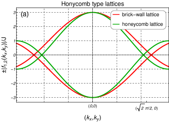
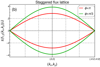
Figure 1: (color online) The tight-binding energy dispersion for (a) the honeycomb type of lattices - standard honeycomb and brick-wall lattices, (b) the staggered flux lattice with $\phi=\pi$ and $\pi/3$. The particular paths in the wave vector space are chosen to show the existence of Dirac points in the tight-binding dispersion, i.e. the points at which dispersions intersects.

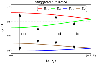
Figure 2: (color online) The wave vector $\mathbf{k}=\left(k_{x},\,k_{y}\right)$ dependence of the quasi-particle and hole energy bands in the MI phase. The staggered flux lattice for $J/U=0.043$ and $\mu=0.414$ is depicted. The arrows show possible transitions in the linear response dynamics considered in this paper. $uu$, $ll$ and $ul$, $lu$ correspond to the intra and inter-band transitions, respectively.

At the end of this section we also give the form of MI Green function $G^{MI}$ (see Eq. (10)) in the Matsubara frequency representation $\omega_{n}$ which will be useful in further calculations, i.e.

$$G^{MI}(\mathbf{k},i\omega_{n})=\left[\begin{array}[]{cc}G_{1,1}^{MI}(\mathbf{k},\omega_{n})&G_{1,2}^{MI}(\mathbf{k},\omega_{n})\\ G_{2,1}^{MI}(\mathbf{k},\omega_{n})&G_{2,2}^{MI}(\mathbf{k},\omega_{n})\end{array}\right],$$ (16)

where diagonal terms $\alpha=\beta$ are

$$G_{\alpha,\beta}^{MI}(\mathbf{k},\omega_{n})$$

$$=\frac{1}{2}\left[\frac{z_{p,u}\left(\mathbf{k}\right)}{i\omega_{n}-E_{p,u}\left(\mathbf{k}\right)}+\frac{1-z_{p,u}\left(\mathbf{k}\right)}{i\omega_{n}-E_{h,u}\left(\mathbf{k}\right)}\right.$$

$$\left.-\frac{z_{p,l}\left(\mathbf{k}\right)}{i\omega_{n}-E_{p,l}\left(\mathbf{k}\right)}-\frac{1-z_{p,l}\left(\mathbf{k}\right)}{i\omega_{n}-E_{h,l}\left(\mathbf{k}\right)}\right],$$ (17)

and off-diagonal terms $\alpha\neq\beta$ are

$$G_{\alpha,\beta}^{MI}(\mathbf{k},\omega_{n})=\frac{f_{\alpha,\beta}(\mathbf{k})}{2\left|f_{\alpha,\beta}(\mathbf{k})\right|}$$

$$\times\left[-\frac{z_{p,u}\left(\mathbf{k}\right)}{i\omega_{n}-E_{p,u}\left(\mathbf{k}\right)}-\frac{1-z_{p,u}\left(\mathbf{k}\right)}{i\omega_{n}-E_{h,u}\left(\mathbf{k}\right)}\right.$$

$$\left.+\frac{z_{p,l}\left(\mathbf{k}\right)}{i\omega_{n}-E_{p,l}\left(\mathbf{k}\right)}+\frac{1-z_{p,l}\left(\mathbf{k}\right)}{i\omega_{n}-E_{h,l}\left(\mathbf{k}\right)}\right].$$ (18)

The corresponding $z_{p,\alpha}\left(\mathbf{k}\right)$ and $E_{p,u/l}\left(\mathbf{k}\right)$ quantities in Eqs. (17)-(18) are

$$z_{p,\alpha}\left(\mathbf{k}\right)=\frac{E_{p,\alpha}\left(\mathbf{k}\right)+\mu+U}{E_{p,\alpha}\left(\mathbf{k}\right)-E_{h,\alpha}\left(\mathbf{k}\right)}\;,$$ (19)

$$E_{p,u/l}\left(\mathbf{k}\right)=\frac{\pm\left|f_{1,2}(\mathbf{k})\right|}{2}-\mu+U\left(n_{0}-\frac{1}{2}\right)\pm\frac{1}{2}\Delta_{u/d}\left(\mathbf{k}\right),$$ (20)

$$\Delta_{u/l}\left(\mathbf{k}\right)=\sqrt{\left|f_{1,2}(\mathbf{k})\right|^{2}\pm 4\left|f_{1,2}(\mathbf{k})\right|U\left(n_{0}+\frac{1}{2}\right)+U^{2}}.$$ (21)

$E_{p,u/l}\left(\mathbf{k}\right)$ and $E_{h,u/l}\left(\mathbf{k}\right)$ are poles of the Green functions in Eqs. (17)-(18), therefore they are interpreted as quasiparticle energies. The $p$ ($h$) index corresponds to the quasiparticle (quasihole) excitation, while $u$ ($l$) corresponds to the upper (lower) band in the tight-binding model. The $u$ and $l$ bands in the tight binding model are obtained from the eigenenergies of $\mathbf{F}(\mathbf{k})$ (Eq. (11)) and are given by $\left|f_{1,2}(\mathbf{k})\right|$ and $-\left|f_{1,2}(\mathbf{k})\right|$, respectively.

An important feature of the lattices considered here is that they exhibit tunable Dirac points. To show this, we plot the tight-binding energy dispersions $\pm\left|f_{1,2}(\mathbf{k})\right|$ of honeycomb and brick-wall lattices in Fig. 1 a and the tight-binding energy dispersions of staggered flux lattice in Fig. 1 b. The corresponding formulas for these dispersions are given in Appendix IV.1. The tunability of the honeycomb like lattice is obtained by modification of its geometry (standard honeycomb geometry and brick-wall geometry) which cause a shift of Dirac points locations in the wave vector space (see Fig. 1 a). This modification also slightly changes the steepness of the relativistic dispersion around Dirac points. Moreover, changing the flux amplitude $\phi$ in the staggered flux lattice implies changes in the steepness of relativistic dispersion around the Dirac points, which is more pronounced than in Fig. 1 a. These effects have direct consequences on the linear response dynamics which will be discussed in the subsequent sections.

Additionally, to show how the excitation spectra of quasiparticles are affected by the Dirac points, we plot the MI energy dispersion of staggered flux lattice in Fig. 2 (the analogous plot can be given for the honeycomb like lattices). In this Figure, the Dirac points are located in the quasiparticle and hole spectrum at $\left(\pi/2,\,\pi/2\right)$ and are separated by energy $U$ (a similar observation was made in the uniform magnetic field Sajna et al. (2014); Sajna and Polak (2014)).

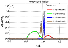
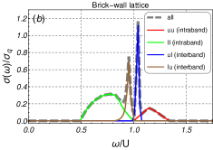
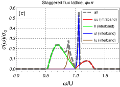
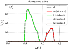
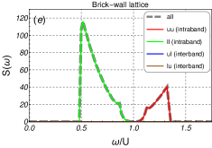
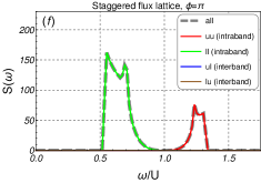
Figure 3: (color online) Frequency $\omega$ dependent conductivity $\sigma(\omega)$ (a-c) and $S(\omega)$ (d-f) in the MI phase at zero temperature. The latter quantity is proportional to the isotropic energy absorption rate. The remaining parameters are $\mu/U=0.414$, $J/U=0.043$. The symbols $uu$, $dd$, $ud$, $du$ correspond to the transitions depicted in Fig. 2. The bold and dashed gray line give the total response of the system coming from the all transitions summed (i.e. from intra and interband transitions); $\sigma_{q}$ denotes the quantum unit of conductance defined in Eq. 33.

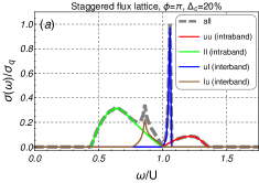
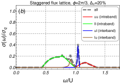
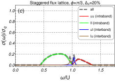
Figure 4: (color online) Frequency dependent conductivity in the MI phase at zero temperature. Staggered flux lattice is considered with the flux amplitudes: (a) $\phi=\pi$, (b) $\phi=2\pi/3$, (c) $\phi=\pi/3$. For clarity, we plot dynamical conductivity with the same absolute detuning of hopping amplitude $J$ from the phase boundary, i.e. $\Delta_{c}=(J_{c}-J)/J_{c}=20\%$ because $J_{c}$ is a $\phi$ dependent function Lim et al. (2008, 2010). In particular (a) $J/U\approx 0.049$, $(J/U)_{c}\approx 0.061$, (b) $J/U\approx 0.040$, $(J/U)_{c}\approx 0.050$, (c) $J/U\approx 0.036$, $(J/U)_{c}\approx 0.044$. The bold and dashed gray line give the total response of the system coming from the all transitions summed (i.e. from intra and interband transitions). The chemical potential is $\mu/U=0.414$.

II.3 Linear response kernel in the MI phase

The linear response kernel for the phase or amplitude modulation perturbation (in the MI phase) can be derived from the following form of the four point correlation function

$$K\left(i\omega\right)$$

$$=\frac{1}{N}\sum_{\mathbf{k},\mathbf{k}^{\prime}}\int_{0}^{\beta}d\tau e^{i\omega\tau}\sum_{\lambda_{1},\lambda_{2},\lambda_{3},\lambda_{4}=1}^{2}\gamma_{\lambda_{1},\lambda_{2}}(\mathbf{k})\gamma_{\lambda_{3},\lambda_{4}}(\mathbf{k}^{\prime})$$

$$\times\left\langle\,b_{\lambda_{1},\mathbf{k}}^{*}(\tau)b_{\lambda_{2},\mathbf{k}}(\tau)\,b_{\lambda_{3},\mathbf{k}^{\prime}}^{*}(0)b_{\lambda_{4},\mathbf{k}^{\prime}}(0)\right\rangle,$$ (22)

where the average $\left\langle...\right\rangle$ is defined over the effective action from Eq.(9) and we assume a translation invariant lattice. Applying the Matsubara frequency transformation for $b$, $b^{*}$ fields, together with the Wick theorem to Eq. (22) one gets

$$K\left(i\omega\right)$$

$$=\frac{1}{\beta N}\sum_{n}\sum_{\mathbf{k}}\sum_{\lambda_{1},\lambda_{2},\lambda_{3},\lambda_{4}=1}^{2}\gamma_{\lambda_{1},\lambda_{2}}^{1}(\mathbf{k})\gamma_{\lambda_{3},\lambda_{4}}^{2}(\mathbf{k})$$

$$\times G_{\lambda_{4},\lambda_{1}}^{MI}(\mathbf{k},\omega_{n})G_{\lambda_{2},\lambda_{3}}^{MI}(\mathbf{k},\omega_{n}+\omega),$$ (23)

in which

$$\left\langle\,b_{\lambda_{\mu},\mathbf{k},n}b_{\lambda_{\nu},\mathbf{k},n}^{*}\right\rangle=G_{\lambda_{\mu},\lambda_{\nu}}^{MI}(\mathbf{k},\omega_{n}),$$ (24)

where the indices $\lambda_{\mu},\lambda_{\nu}\in\left\{1,2\right\}$ denote the matrix element of MI Green function which is the $2$ by $2$ matrix defined in Eq. (10).

Careful explanation of the form of $K\left(i\omega\right)$ in Eq. (22) is needed. Firstly, it describes the paramagnetic part of linear response in MI phase for which $\omega>0$. Secondly, the form of $K\left(i\omega\right)$ depends on the form of the considered external perturbation. In this work, we consider two quantities: $\sigma\left(\omega\right)$ and $S\left(\omega\right)$. The symbol $\sigma\left(\omega\right)$ denotes the dynamical conductivity and is defined by the current autocorrelation function Kampf and Zimanyi (1993). The function $S\left(\omega\right)$ is proportional to the isotropic energy absorption rate and is defined by the kinetic energy autocorrelation function Huber et al. (2007); Pollet and Prokof’ev (2012). It is important to stress here that $\sigma\left(\omega\right)$ and $S\left(\omega\right)$ are also related with the response of the system to the phase and the amplitude periodic modulation of the optical lattice, respectively Huber et al. (2007); Pollet and Prokof’ev (2012); Tokuno and Giamarchi (2011). Namely, within the notation introduced in Sec. II.2, the optical conductivity can be obtained from

$$\sigma\left(\omega\right)=\left.\frac{e_{eff}^{2}}{\omega}K\left(i\omega\right)\right|_{i\omega\rightarrow\omega+i0^{+}},$$ (25)

where

$$\gamma_{\lambda_{1},\lambda_{2}}^{1}(\mathbf{k})=\gamma_{\lambda_{1},\lambda_{2}}^{2}(\mathbf{k})=\partial_{k_{x}}f{}_{\lambda_{1},\lambda_{2}}(\mathbf{k}),$$ (26)

and $e_{eff}$ is the effective charge (which in the optical lattice can be generated e.g. by the synthetic gauge field). The expression $i\omega\rightarrow\omega+i0^{+}$ denotes the analytic continuation and $f{}_{\lambda_{1},\lambda_{2}}(\mathbf{k})$ is the $(\lambda_{1},\lambda_{2})$ matrix element of $\mathbf{F}(\mathbf{k})$ from Eq. (11). Partial derivative over $k_{x}$ in Eq. (26) means that $xx$ component of the longitudinal conductivity is considered. The form of Eq. (25) agrees with those ound in literature Kampf and Zimanyi (1993); Sajna et al. (2014); Grygiel et al. (2017).

In the case of $S(\omega)$ one gets

$$S\left(\omega\right)=\textrm{Im}\left[\left.K\left(i\omega\right)\right|_{i\omega\rightarrow\omega+i0^{+}}\right],$$ (27)

where

$$\gamma_{\lambda_{1},\lambda_{2}}^{1}(\mathbf{k})=\gamma_{\lambda_{1},\lambda_{2}}^{2}(\mathbf{k})=f{}_{\lambda_{1},\lambda_{2}}(\mathbf{k}).$$ (28)

$S\left(\omega\right)$ has been previously studied in different contexts, e.g. correlated fermions Kollath et al. (2006b), Higgs mode Pollet and Prokof’ev (2012) or thermometry in MI phase Sajna (2016).

Because we are focused on the MI phase, one can give the general form of $K\left(i\omega\right)$ by using Eqs. (23) and (17)-(21), i.e.

$$K\left(i\omega\right)$$ (29)

$$=\frac{1}{N}\sum_{\mathbf{k}}\sum_{\alpha,\beta\in\{u,l\}}\Gamma_{\alpha\beta}^{\gamma}\left(\mathbf{k}\right)\frac{\left[1-z_{p,\alpha}\left(\mathbf{k}\right)\right]z_{p,\beta}\left(\mathbf{k}\right)}{E_{h,\alpha}\left(\mathbf{k}\right)+i\hbar\omega-E_{p,\beta}\left(\mathbf{k}\right)},$$ (30)

where

$$\Gamma_{uu}^{\gamma}\left(\mathbf{k}\right)=\Gamma_{ll}^{\gamma}\left(\mathbf{k}\right)=$$

$$=\left(\frac{\gamma_{2,1}^{1}\left(\mathbf{k}\right)f{}_{1,2}\left(\mathbf{k}\right)+\gamma_{1,2}^{1}\left(\mathbf{k}\right)\bar{f}_{1,2}\left(\mathbf{k}\right)}{2\left|f_{1,2}\left(\mathbf{k}\right)\right|}\right)^{2},$$ (31)

$$\Gamma_{ul}^{\gamma}\left(\mathbf{k}\right)=\Gamma_{lu}^{\gamma}\left(\mathbf{k}\right)$$

$$=-\left(\frac{\gamma_{1}^{2,1}\left(\mathbf{k}\right)f{}_{1,2}\left(\mathbf{k}\right)-\gamma_{1}^{1,2}\left(\mathbf{k}\right)\bar{f}_{1,2}\left(\mathbf{k}\right)}{2\left|f_{1,2}\left(\mathbf{k}\right)\right|}\right)^{2},$$ (32)

and weights $\Gamma_{uu}^{\gamma}$, $\Gamma_{ll}^{\gamma}$ and $\Gamma_{ul}^{\gamma}$, $\Gamma_{lu}^{\gamma}$ correspond to the intra and inter-band transitions depicted in Fig. (2) for which a more detailed discussion will be given shortly (the $\gamma$ index is reserved for conductivity $\Gamma_{\alpha\beta}^{cond}$ and for energy absorption rate $\Gamma_{\alpha\beta}^{abs}$). Moreover, in derivation of Eqs. (29)-(32) we assume a zero temperature limit and for simplicity we identify $\gamma^{1}$ with $\gamma^{2}$ i.e. $\gamma^{1}=\gamma^{2}$ which agrees with Eqs. (26) and (28).

It is also worth pointing out here that Eqs. (29-32) are valid for an arbitrary form of the staggered symmetry introduced by the hopping amplitude $\mathbf{F}(\mathbf{k})$ (see Eq. (11)) and therefore, these results are not restricted to the lattices considered here (i.e. for the lattices defined by Eqs. (13)-(15)).

II.4 Dynamical conductivity

To calculate the dynamical (longitudinal) conductivity $\sigma(\omega)$ from Eq. (25), the analytic continuation of $K\left(i\omega\right)/\omega$ is needed ($i\omega\rightarrow\omega+i0^{+}$). This yields the following form of $xx$ component of the longitudinal conductivity

$$\textrm{Re}\sigma\left(\omega\right)$$

$$=\sigma_{q}\frac{2\pi^{2}}{N}\sum_{\mathbf{k}}\sum_{\alpha,\beta\in\{u,l\}}\Gamma_{\alpha\beta}^{cond}\left(\mathbf{k}\right)\frac{\left[1-z_{p,\alpha}\left(\mathbf{k}\right)\right]z_{p,\beta}\left(\mathbf{k}\right)}{E_{h,\alpha}\left(\mathbf{k}\right)-E_{p,\beta}\left(\mathbf{k}\right)}$$

$$\times\delta\left(\omega-\left[E_{p,\beta}\left(\mathbf{k}\right)-E_{h,\alpha}\left(\mathbf{k}\right)\right]\right),$$ (33)

where we focus on the real part of dynamical conductivity, i.e. $\textrm{Re}\sigma\left(\omega\right)$ and we define $\sigma_{q}=e_{eff}^{2}/h$ as a quantum unit of conductance Sajna et al. (2014). From the form of $\textrm{Re}\sigma\left(\omega\right)$, we see that the response of the system appears at the energy difference between quasiparticle ($E_{p,\beta}\left(\mathbf{k}\right)$) and hole excitations ($E_{h,\alpha}\left(\mathbf{k}\right)$) through the Dirac delta function $\delta$. Therefore for two band models in the MI phase, one can have four types of excitations. The transitions corresponding to these excitations are schematically drawn in Fig. (2). In general, one can divide such transitions into two classes which have intra ($uu$, $ll$) or interband ($ul$, $lu$) character. The intraband transitions are mostly responsible for the lowest and highest energy excitations and e.g. they can describe remarkable phenomenon like the finite critical conductivity Fisher et al. (1990); Kampf and Zimanyi (1993); Cha and Girvin (1994); Sajna et al. (2014). The interband transitions are responsible for intermediate behavior and in the cases considered in this work, they strongly modify the response around the energy scales in which the Dirac points appear (a similar behavior has been very recently reported in the uniform magnetic fields Grygiel et al. (2017) when this work was finalized).

Next, calculating the conductivity coefficients $\Gamma_{\alpha\beta}^{cond}$ in Eqs. (33) by using Eqs. (31)-(32) and (26) one gets

$$\Gamma_{uu}^{cond}\left(\mathbf{k}\right)=\Gamma_{ll}^{cond}\left(\mathbf{k}\right)=\left(\partial_{k_{x}}\left|f_{1,2}\left(\mathbf{k}\right)\right|\right)^{2},$$ (34)

$$\Gamma_{ul}^{cond}\left(\mathbf{k}\right)=\Gamma_{lu}^{cond}\left(\mathbf{k}\right)=$$

$$=-\left(\frac{f{}_{1,2}(\mathbf{k})\partial_{k_{x}}\bar{f}{}_{1,2}(\mathbf{k})-\bar{f}_{1,2}(\mathbf{k})\partial_{k_{x}}f{}_{1,2}(\mathbf{k})}{2\left|f_{1,2}\left(\mathbf{k}\right)\right|}\right)^{2}.$$ (35)

From the above equations, we see that all four transitions ($uu$, $ll$, $ul$, $lu$) can contribute to the conductivity. However, to consider a particular lattice, explicit forms of the functions $\Gamma_{\alpha\beta}^{cond}$ have to be given together with the remaining functions in Eq. (33).

To show how the intra ($uu$, $ll$) and interband ($ul$, $lu$) transitions behave in the lattices with staggered symmetry, we consider at first the honeycomb type of lattices (see Eqs. (14) and (15)). For standard honeycomb lattice one gets

$$\Gamma_{uu}^{cond}\left(\mathbf{k}\right)=\Gamma_{ll}^{cond}\left(\mathbf{k}\right)=3J^{4}\sin^{2}\left(\frac{\sqrt{3}}{2}k_{x}\right)$$

$$\times\left(\frac{2\cos\left(\frac{\sqrt{3}}{2}k_{x}\right)+\cos\left(\frac{3}{2}k_{y}\right)}{\left|f_{1,2}^{hc}\left(\mathbf{k}\right)\right|}\right)^{2},$$ (36)

$$\Gamma_{ul}^{cond}\left(\mathbf{k}\right)=\Gamma_{lu}^{cond}\left(\mathbf{k}\right)=\frac{3J^{4}\sin^{2}\left(\frac{\sqrt{3}}{2}k_{x}\right)\sin^{2}\left(\frac{3}{2}k_{y}\right)}{\left|f_{1,2}^{hc}\left(\mathbf{k}\right)\right|^{2}},$$ (37)

and for brick-wall lattice

$$\Gamma_{uu}^{cond}\left(\mathbf{k}\right)=\Gamma_{ll}^{cond}\left(\mathbf{k}\right)=4J^{4}\sin^{2}\left(k_{x}\right)$$

$$\times\left(\frac{2\cos\left(k_{x}\right)+\cos\left(k_{y}\right)}{\left|f_{1,2}^{bw}\left(\mathbf{k}\right)\right|}\right)^{2},$$ (38)

$$\Gamma_{ul}^{cond}\left(\mathbf{k}\right)=\Gamma_{lu}^{cond}\left(\mathbf{k}\right)=\frac{4J^{4}\sin^{2}\left(k_{x}\right)\sin^{2}\left(k_{y}\right)}{\left|f_{1,2}^{bw}\left(\mathbf{k}\right)\right|^{2}},$$ (39)

where we set the lattice constant $a$ to one. It is straightforward to see that the above formulas for honeycomb and brick-wall lattices, have a similar form (see also Eqs. (14) and (15)) which result in similar behavior of dynamical conductivity - Figs. 3 a and b. In these Figures one sees that interband transitions ($ul$, $lu$), which appear near the Dirac point, are more pronounced than the intraband transitions ($uu$, $ll$) (Dirac point is visible as a vanishing of conductivity at $\omega=U$). Similar behavior of significant differences in the intra and interband transition amplitudes has been very recently reported also for the uniform magnetic field Grygiel et al. (2017). Moreover, the shifting of Dirac points in the wave vector space $\mathbf{k}$ (Fig. 1 a), slightly changed the interband transitions amplitude, i.e. the brick-wall interband transitions had slightly higher amplitudes than the corresponding transitions for the honeycomb lattice. Therefore, the modification of the lattice geometry had a direct consequence on the linear response dynamics near the Dirac points.

We can achieve much more pronounced tuning of the dynamics near the Dirac points if we consider the staggered flux lattice. Prior to showing this, let us first write the coefficients $\Gamma_{\alpha\beta}^{cond}$ for this type of lattice:

$$\Gamma_{uu}^{cond}\left(\mathbf{k}\right)=\Gamma_{ll}^{cond}\left(\mathbf{k}\right)=16J^{4}\sin^{2}\left(k_{x}a\right)$$

$$\times\left(\frac{\cos\left(k_{x}a\right)+\cos\left(\phi/2\right)\cos\left(k_{y}a\right)}{\left|f_{1,2}^{flux}\left(\mathbf{k}\right)\right|}\right)^{2},$$ (40)

$$\Gamma_{ul}^{cond}\left(\mathbf{k}\right)=\Gamma_{lu}^{cond}\left(\mathbf{k}\right)=$$

$$=\frac{4J^{4}\sin^{2}\left(k_{x}a\right)\cos^{2}\left(k_{y}a\right)\sin^{2}\left(\phi/2\right)}{\left|f_{1,2}^{flux}\left(\mathbf{k}\right)\right|^{2}}.$$ (41)

From the above equations, we see that the interband coefficients, i.e. $\Gamma_{ul}^{cond}\left(\mathbf{k}\right)$ and $\Gamma_{lu}^{cond}\left(\mathbf{k}\right)$, depend on the square power of the $\sin\left(\phi/2\right)$ function. This explains why the interband transitions are the largest for $\phi=\pi$ and they vanish in the limit $\phi\rightarrow 0$ (for $\phi=0$ the square lattice limit is recovered where interband transitions do not exist Sajna et al. (2014)). We prove this remarkable behavior of interband transitions by plotting the dynamical conductivity for different values of $\phi$ amplitude in Fig. 4. It is important to point out here that such a behavior is directly connected to the steepness of tight-binding dispersion near the Dirac points which is tuned with a different $\phi$ amplitude, see Fig. 1 b.

Moreover, it is very instructive to explain why the interband transitions ($ul$, $lu$) appear around the Dirac points (i.e. around $\omega=U$) (see Figs. 3 a-b). If we look at Fig. 2, we see that the bandwidth of qasiparticle excitations is by about twice larger than the quasihole band. This can be simply accounted for by the different effective hoppings of particles and holes and e.g. for free bosonic case it is simply $(n_{0}+1)J$ and $n_{0}J$, respectively (see, e.g., Yanay and Mueller (2016); Aichhorn et al. (2008)). Therefore, moving away from the Dirac points which for staggered flux lattice are at $(\pm\pi/2,\pm\pi/2)$ (see also Fig. 2), we see that the $ul$ and $lu$ transitions for a given $\mathbf{k}$ vary slightly from the interaction energy $U$ because of the different effective hoppings of particles and holes. We conclude, that exactly this difference in the effective hoppings, gives rise to the linear response dynamics which concentrates around the Dirac points. A corresponding situation can be also found for the honeycomb type of lattices.

II.5 Isotropic energy absorption rate

In Sec. II.4 we have shown how the interband transitions can be engineered by the lattice geometry or staggered flux. Here, we show that such a manipulation of transitions in the strongly correlated bosonic system can be also achieved in a much robust way, i.e. by a suitable choice of external perturbation. Dynamical conductivity considered in the previous section is related to the periodic phase modulation of the optical lattice Tokuno and Giamarchi (2011). Now we show what happens if we consider the periodic amplitude lattice modulation which is directly connected to the function $S(\omega)$ (Eq. (27)) Kollath et al. (2006b); Huber et al. (2007); Pollet and Prokof’ev (2012).

Namely, we consider $S(\omega)$ which is proportional to the isotropic energy absorption rate and is defined in Eqs. (27)-(32). After analytical calculations one gets

$$S\left(\omega\right)$$

$$=\frac{\pi}{N}\sum_{\mathbf{k}}\sum_{\alpha,\beta\in\{u,l\}}\Gamma_{\alpha\beta}^{cond}\left(\mathbf{k}\right)\left[1-z_{p,\alpha}\left(\mathbf{k}\right)\right]z_{p,\beta}\left(\mathbf{k}\right)$$

$$\times\delta\left(\omega-\left[E_{p,\beta}\left(\mathbf{k}\right)-E_{h,\alpha}\left(\mathbf{k}\right)\right]\right),$$ (42)

where

$$\Gamma_{uu}^{abs}\left(\mathbf{k}\right)=\Gamma_{ll}^{abs}\left(\mathbf{k}\right)=\left(\left|f_{1,2}\left(\mathbf{k}\right)\right|\right)^{2},$$ (43)

$$\Gamma_{ul}^{abs}\left(\mathbf{k}\right)=\Gamma_{lu}^{abs}\left(\mathbf{k}\right)=0,$$ (44)

and where the $\left|f_{1,2}\left(\mathbf{k}\right)\right|$ function is the tight-binding energy dispersion of the lattices considered in this work (see, Eqs (45)-(47)). The result of Eq. (44) is especially interesting. It says that interband transtions ($ul$, $lu$) are completely turned off in the isotropic and periodic modulation of the lattice amplitude for the lattices with staggered symmetry introduced by the hopping amplitude (see Eq. (11). We confirm this analytical result, by plotting Eqs. (42)-(44) in Figs. 3 d, e and f for the honeycomb, brick-wall and staggered flux lattice, respectively. These plots should be compared with the conductivity $\sigma(\omega)$ plots, Figs. 3 a, b and c, for which the interband transitions are present (for $\sigma(\omega)$ the interband weights $\Gamma_{ul}^{cond}$ and $\Gamma_{lu}^{cond}$ do not vanish identically like for the $S(\omega)$ case, compare Eqs. (35) and (44)).

III Summary

In this work we have considered linear response dynamics in the MI phase for the lattices with staggered symmetry. This symmetry was introduced by the hopping amplitude and takes into account a broad class of lattice currently realized in the optical lattice systems. We have focused on the lattices which contain Dirac points in their tight-binding energy dispersions and which can allow Dirac like physics engineering.

As the main result of our considerations we have shown that linear response dynamics around the Dirac points can be highly tuned by a suitable type of the external perturbation or by modification of the lattice parameters. This shows that the interband transitions can be very sensitive to the particular experiment realization and can be a signature for emergence of relativistic dynamics related with the Dirac points.

Moreover, we have explained that such a peculiar dynamics around the Dirac points is directly connected to the effective hopping energies for holes and particles. This further can provide an indirect proof of the non-equal values of bandwidth for quasiparticle and hole excitations in the MI phase.

It is also important to stress here that presented theoretical framework can be directly applied to the other lattice systems showing the staggered lattice symmetry.

IV Appendix

IV.1 Tight-binding energy dispersions

Tight-binding energy dispersions which are plotted in Fig. 1 have the following forms:

- for honeycomb lattice

$$\left|f_{1,2}^{hc}\left(\mathbf{k}\right)\right|=\pm J\sqrt{1+4\cos^{2}\left(\frac{\sqrt{3}}{2}k_{x}a\right)+4\cos\left(\frac{\sqrt{3}}{2}k_{x}a\right)\cos\left(\frac{3}{2}k_{y}a\right)},$$ (45)

- for brick-wall lattice

$$\left|f_{1,2}^{bw}\left(\mathbf{k}\right)\right|=\pm J\sqrt{1+4\cos^{2}\left(k_{x}a\right)+4\cos\left(k_{x}a\right)\cos\left(k_{y}a\right)},$$ (46)

- for staggered flux lattice

$$\left|f_{1,2}^{flux}\left(\mathbf{k}\right)\right|=\pm 2J\sqrt{\cos^{2}\left(k_{x}a\right)+\cos^{2}\left(k_{y}a\right)+2\cos\left(\frac{\phi}{2}\right)\cos\left(k_{x}a\right)\cos\left(k_{y}a\right)},$$ (47)

where $a$ is the lattice constant.

References

- Stöferle et al. (2004) T. Stöferle, H. Moritz, C. Schori, M. Köhl, and T. Esslinger, Phys. Rev. Lett. 92, 130403 (2004).
- Schori et al. (2004) C. Schori, T. Stöferle, H. Moritz, M. Köhl, and T. Esslinger, Phys. Rev. Lett. 93, 240402 (2004).
- Reischl et al. (2005) A. Reischl, K. P. Schmidt, and G. S. Uhrig, Phys. Rev. A 72, 063609 (2005).
- Kollath et al. (2006a) C. Kollath, A. Iucci, T. Giamarchi, W. Hofstetter, and U. Schollwöck, Phys. Rev. Lett. 97, 050402 (2006a).
- Iucci et al. (2006) A. Iucci, M. A. Cazalilla, A. F. Ho, and T. Giamarchi, Phys. Rev. A 73, 041608 (2006).
- Huber et al. (2007) S. D. Huber, E. Altman, H. P. Büchler, and G. Blatter, Phys. Rev. B 75, 085106 (2007).
- Tokuno and Giamarchi (2011) A. Tokuno and T. Giamarchi, Phys. Rev. Lett. 106, 205301 (2011).
- Huo et al. (2011) J.-W. Huo, F.-C. Zhang, W. Chen, M. Troyer, and U. Schollwöck, Phys. Rev. A 84, 043608 (2011).
- Mark et al. (2011) M. J. Mark, E. Haller, K. Lauber, J. G. Danzl, A. J. Daley, and H.-C. Nägerl, Phys. Rev. Lett. 107, 175301 (2011).
- Endres et al. (2012) M. Endres, T. Fukuhara, D. Pekker, M. Cheneau, P. Schau, C. Gross, E. Demler, S. Kuhr, and I. Bloch, Nature 487, 454 (2012).
- Łącki et al. (2012) M. Łącki, D. Delande, and J. Zakrzewski, Phys. Rev. A 86, 013602 (2012).
- Pollet and Prokof’ev (2012) L. Pollet and N. Prokof’ev, Phys. Rev. Lett. 109, 010401 (2012).
- zu Münster et al. (2014) K. zu Münster, F. Gebhard, S. Ejima, and H. Fehske, Phys. Rev. A 89, 063623 (2014).
- Strand et al. (2015) H. U. R. Strand, M. Eckstein, and P. Werner, Phys. Rev. A 92, 063602 (2015).
- Liu et al. (2015) L. Liu, K. Chen, Y. Deng, M. Endres, L. Pollet, and N. Prokof’ev, Phys. Rev. B 92, 174521 (2015).
- Sajna (2016) A. S. Sajna, Phys. Rev. A 94, 043612 (2016).
- Goldman et al. (2014) N. Goldman, G. Juzeliūnas, P. Öhberg, and I. B. Spielman, Reports on Progress in Physics 77, 126401 (2014).
- Tarruell et al. (2012) L. Tarruell, D. Greif, T. Uehlinger, G. Jotzu, and T. Esslinger, Nature 483, 302 (2012).
- Windpassinger and Sengstock (2013) P. Windpassinger and K. Sengstock, Rep. Prog. Phys. (2013).
- Grygiel et al. (2017) B. Grygiel, K. Patucha, and T. A. Zaleski, Phys. Rev. B 96, 094520 (2017).
- Sajna et al. (2014) A. S. Sajna, T. P. Polak, and R. Micnas, Phys. Rev. A 89, 023631 (2014).
- Sajna and Polak (2014) A. S. Sajna and T. P. Polak, Phys. Rev. A 90, 043603 (2014).
- Sajna et al. (2015) A. Sajna, T. Polak, and R. Micnas, Acta Physica Polonica A 127, 448 (2015).
- Grygiel et al. (2016) B. Grygiel, K. Patucha, and T. Zaleski, Acta Physica Polonica A 130, 633 (2016).
- Lim et al. (2010) L.-K. Lim, A. Hemmerich, and C. M. Smith, Phys. Rev. A 81, 23404 (2010).
- Lim et al. (2008) L.-K. Lim, C. M. Smith, and A. Hemmerich, Phys. Rev. Lett. 100, 130402 (2008).
- Abanin et al. (2013) D. A. Abanin, T. Kitagawa, I. Bloch, and E. Demler, Phys. Rev. Lett. 110, 165304 (2013).
- Fisher et al. (1989) M. P. A. Fisher, P. B. Weichman, G. Grinstein, and D. S. Fisher, Phys. Rev. B B40, 546 (1989).
- Gersch and Knollman (1963) H. A. Gersch and G. C. Knollman, Phys. Rev. 129, 959 (1963).
- Stoof et al. (2009) H. T. C. Stoof, K. B. Gubbels, and D. B. M. Dickerscheid, Ultracold Quantum Fields (Springer, 2009).
- Sengupta and Dupuis (2005) K. Sengupta and N. Dupuis, Phys. Rev. A 71, 033629 (2005).
- Kampf and Zimanyi (1993) A. P. Kampf and G. T. Zimanyi, Phys. Rev. B 47, 279 (1993).
- Kollath et al. (2006b) C. Kollath, A. Iucci, I. P. McCulloch, and T. Giamarchi, Phys. Rev. A 74, 041604 (2006b).
- Fisher et al. (1990) M. P. A. Fisher, G. Grinstein, and S. M. Girvin, Phys. Rev. Lett. 64, 587 (1990).
- Cha and Girvin (1994) M.-C. Cha and S. M. Girvin, Phys. Rev. B 49, 9794 (1994).
- Yanay and Mueller (2016) Y. Yanay and E. J. Mueller, Phys. Rev. A 93, 013622 (2016).
- Aichhorn et al. (2008) M. Aichhorn, M. Hohenadler, C. Tahan, and P. B. Littlewood, Phys. Rev. Lett. 100, 216401 (2008).