Photometric characterization of the Dark Energy Camera

Abstract

We characterize the variation in photometric response of the Dark Energy Camera (DECam) across its 520 Mpix science array during 4 years of operation. These variations are measured using high signal-to-noise aperture photometry of $>10^{7}$ stellar images in thousands of exposures of a few selected fields, with the telescope dithered to move the sources around the array. A calibration procedure based on these results brings the RMS variation in aperture magnitudes of bright stars on cloudless nights down to 2–3 mmag, with $<1$ mmag of correlated photometric errors for stars separated by $\geq 20\arcsec.$ On cloudless nights, any departures of the exposure zeropoints from a secant airmass law exceeding $>1$ mmag are plausibly attributable to spatial/temporal variations in aperture corrections. These variations can be inferred and corrected by measuring the fraction of stellar light in an annulus between 6″ and 8″ diameter. Key elements of this calibration include: correction of amplifier nonlinearities; distinguishing pixel-area variations and stray light from quantum-efficiency variations in the flat fields; field-dependent color corrections; and the use of an aperture-correction proxy. The DECam response pattern across the 2° field drifts over months by up to $\pm 7$ mmag, in a nearly-wavelength-independent low-order pattern. We find no fundamental barriers to pushing global photometric calibrations toward mmag accuracy.

1 Introduction

Photometric calibration of sources in an astronomical imaging survey requires ensuring that the flux assigned to a given (non-variable) source would be the same regardless of where on the detector array it is imaged, where that source lies on the sky, or when the exposure was taken. The success of the resultant calibration therefore depends on our ability to model the response of the detector/optics/atmosphere combination across the focal plane, and the nature and time scales of variations in this response. In this work, we perform these characterizations for the Dark Energy Camera (Flaugher et al., 2015, DECam), a CCD imager with 520 megapixel science array in operation on the 4-meter Blanco telescope since late 2012. Increasing precision and homogeneity of photometric calibration leads to better science results across a broad range of astrophysical topics pursued by the Dark Energy Survey (DES) and other projects using DECam: stellar populations and dust distributions in the Milky Way and its satellites; high-accuracy galaxy clustering and photometric redshift measurements; studies of stellar and quasar variability over the 5-year time span of DES; and accurate Hubble diagrams of supernova flux vs redshift.

We concentrate here on relative photometric calibration, i.e. placing all of the camera’s observations on a consistent flux scale. Absolute calibration, i.e. determination of the normalization of this unified flux scale, requires observations of some celestial or terrestrial sources of known flux, and we defer this discussion to a future publication. The traditional approach to relative photometry in the visible/near-IR, from the days of single-channel photometers, was to interleave observations of “standard” stars of known flux with observations of targets. The standards are used to establish the parameters of a parametric atmosphere$+$instrument response model for count rates vs source flux, and then invert this relation to establish fluxes for the targets. The success of this approach (as well as the ability to establish the standard-star network to begin with) rests on a critical assumption, namely: the response (including atmospheric transmission) is invariant, to the desired photometric precision, on the time scale of the observations used to establish and use its parametric model. We will refer to this assumption of slowly-varying atmospheric transparency (and instrument response) as the “atmospheric prior” on our photometric calibration. This assumption is easily violated on nights with clouds. In this paper we will only examine data taken on cloudless, a.k.a. “photometric” nights, as indicated by the absence of any clouds on images from the RASICAM thermal-IR all-sky monitor (Reil et al., 2014). See Burke et al. (2014) for discussion of the spatial and temporal structure of cloud extinction.

With the advent of large-format array detectors and the ability to perform quantitative imaging for large numbers of stars simultaneously, the photometric calibration task gains a critical new responsibility and a critical new tool. The responsibility is to determine the relative response of pixels across the array. Since the earliest days of CCD astronomy this has been done by imaging a near-Lambertian source (either sky background or a dome screen) to generate a “dome flat” image that is assumed to reflect the relative response to stellar illumination across the array. As detailed in Bernstein et al. (2017b) and summarized below, the dome flat technique contains several flaws that preclude its use for deriving the true photometric response of the array at percent-level precision (10 mmag) or better. Fortunately, the new tool offered by array observations is internal consistency: the constraint that repeat observations of a given source should yield the same flux. Simple applications of the internal consistency constraint to derive a parametric model of array response involved scanning a single source across the array (Manfroid, 1995; McLeod et al., 1995). The first application to survey-scale data, using many stellar images per exposure, was on the Sloan Digital Sky Survey (SDSS), by Padmanabhan et al. (2008). The DES and the future Large Scale Synoptic Survey (LSST) choose survey strategies designed to produce exposures which are highly interlaced in sky position and in time, to better stabilize photometric solutions based on internal consistency. This success rests on the second critical assumption of photometric calibrations, namely that most individual stars have invariant flux, and the median variation in flux of a collection of stars is zero.

It remains true, however, that internal consistency alone is insufficient to fully calibrate a survey. Low-frequency modes of calibration error produce weak magnitude differences between overlapping (i.e. nearby) exposures, which are hence hard to detect and suppress with internal constraints. The atmospheric prior ties down large-scale modes if the survey strategy produces exposures spanning large angles within time intervals shorter than the stability period. Thus the best photometric calibration will combine internal consistency constraints with an atmospheric prior. In this paper we answer several questions that are prerequisite to executing such a calibration of the full survey:

1. What parametric model(s) suffice to homogenize the stellar photometry across the DECam field of view (FOV) in a single exposure?

2. How stable is the atmospheric transmission within a single cloudless night? What physical processes are responsible for any variation and how well can they be modeled and corrected?

3. How does the instrumental response change over intervals between 24 hours and years? What models and parameters are needed to track any variations?

With the answers to these questions in hand, we can proceed to design the optimal calibration system for DES (and for other observations made with DECam), which should inform calibration procedures for other present and future large-FOV imagers.

Photometric calibration of the first-year DES observations is described by Drlica-Wagner et al. (2017). This used the standard technique of nightly zeropoint/color/extinction solutions using a standard-star network, incorporating early versions of the “star flats” described in this paper to flatten individual exposures, and assigning zeropoints to non-photometric exposures by forcing agreement with exposures taken in clear conditions. The RMS magnitude difference between distinct exposures of a given region is $\approx 3$ mmag, after averaging all the stars in a CCD-sized region ($\approx 10\arcmin$). RMS differences between this DES Y1 calibration and magnitudes constructed from APASS Henden & Munari (2014) and 2MASS Skrutskie et al. (2006) is $\approx 20$ mmag, which serves as an upper limit to the errors in the DES Y1 calibration. Using the first three years of DES observations, Burke et al. (2017) present a first foray into joint atmospheric/instrumental photometric calibration, using some of the star-flat calibrations described in this paper and a physical model for atmospheric extinction. Reproducibility of stellar photometry at 5–6 mmag RMS is achieved, and uniformity of the calibration across the 5000 deg² DES footprint is estimated at 7 mmag. Finkbeiner et al. (2016) present a cross-calibration of the SDSS and Pan-Starrs1 (PS1) surveys yielding RMS deviations between the two at similar level. This indicates the current state of the art in photometric calibration of large-scale ground-based sky surveys. Our goal is to understand the photometric behavior of DECam at $\approx 1$ mmag RMS level, in hopes of approaching this level of global calibration accuracy for individual stars in future reductions. We will therefore ignore effects which are expected to cause photometric inaccuracies below this level.

Section 2 first recaps the derivations in Bernstein et al. (2017b) of the operations necessary to convert raw detector outputs into homogeneous stellar flux estimates. Then we describe the formulae and algorithms used to derive the best parametric model of DECam instrumental response. Section 3 describes the data used to derive the DECam photometric model, the code used to process it, and the best-fitting models for DECam instrumental response, and then evaluates their performance in homogenizing short (1-hour) stretches of exposures. Section 4 addresses the question of just how stable a photometric night is, and Section 5 examines the longer-term variation in DECam response. Section 6 evaluates the overall level of our understanding of DECam photometric response, and its implications for calibration accuracy of DES and other contemporary ground-based visible sky surveys.

2 Deriving a response model

2.1 Array response and star flats

The raw digital values produced by DECam for the signal at pixel location $x$ in an exposure labeled by index $t$ need to undergo several detrending steps before we can extract an estimate of the top-of-the-atmosphere flux $f$ of some star in the image. Bernstein et al. (2017b) detail the steps needed to transform the raw data into an image ${\rm Rate}_{\star}({\bf x},t)$ giving the rate of photocarrier production in pixel ${\bf x}$ by celestial objects during exposure $t$. We will adopt the notation of Bernstein et al. (2017b) whereby boldface quantities are vectors over an implied pixel argument ${\bf x},$ and all mathematical operations are assumed to be element-wise over pixels. The steps in the transformation of raw camera data into $\mbox{${\bf Rate}$}_{\star}(t)$ include debiasing, conversion from ADU to photocarriers, linearization of amplifier response, correction of the “brighter-fatter effect” (Antilogus et al., 2014; Gruen et al., 2015), and background subtraction. We refer to Bernstein et al. (2017b) for descriptions of these detrending steps, though the linearization and background-subtraction steps will enter into our analysis of the accuracy of our DECam photometric model.

A single star with flux $f$ and spectral shape $F_{p}(\lambda)$ defined by some parameter(s) $p$ produce photocarriers at the rate

$$\mbox{${\bf Rate}$}_{\star}(t)=\frac{\Omega_{0}}{f_{1}}\mbox{\boldmath$\Omega$}\int d\lambda\,r_{\rm ref}(\lambda)\mbox{${\bf r}$}(\lambda,t)\frac{fF_{p}(\lambda)\mbox{${\bf PSF}$}(\lambda,t)}{\Omega_{0}}.$$ (1)

We define:

• $\Omega_{0}$ as the nominal solid angle of an array pixel, and $\Omega$ as the fractional deviation of each pixel’s size from this value, assumed to be independent of wavelength $\lambda$ across a given filter band.

• $r_{\rm ref}(\lambda)$ as the reference response, the spectral response of a typical pixel in typical atmospheric conditions, otherwise known as the “natural passband” for the chosen filter.

• $\mbox{${\bf r}$}(\lambda,t)$ as the spectral response function giving the true response at a given array position and time relative to the reference response.

• The fraction under the integral gives the apparent surface brightness produced by the star, which is defined by the point spread function $\mbox{${\bf PSF}$}(\lambda,t)$ at the location and time of the exposure of the star.

• $f_{1}$ as the flux of a star that produces 1 charge per second in nominal conditions. We will not be concerned with determination of this constant, which sets the absolute calibration of the photometry.

We opt to normalize these quantities such that

$$\sum_{x}\mbox{${\bf PSF}$}(\lambda,t)\mbox{\boldmath$\Omega$} =1,$$ (2)

$$\int d\lambda\,F_{p}(\lambda)r_{\rm ref}(\lambda) =1.$$ (3)

The units of $F_{p}$ are (wavelength)^-1, and the stellar flux $f$ is then in units of power per unit area. We will also assume that the PSF is wavelength-independent within any particular filter band.

Extraction of the stellar flux from the ${\bf Rate}$ image begins with defining a reference spectrum $F_{\rm ref}(\lambda)$, from which we can define the reference flat field

$$\mbox{${\bf r}$}(t)\equiv\int d\lambda\,F_{\rm ref}(\lambda)\mbox{${\bf r}$}(\lambda,t).$$ (4)

With these definitions, one can show that an estimator for the flux $f_{\alpha t}$ for star $\alpha$ in exposure $t$ can be produced by summing over the pixels $x$ in an aperture around the star:

$$\sum_{x\in\alpha}\frac{\mbox{${\bf Rate}$}_{\star}(t)}{\mbox{${\bf r}$}(t)} =\frac{f_{\alpha t}}{f_{1}}\mbox{${\bf C}$}(t;p)\eta(t),$$ (5)

$$\mbox{${\bf C}$}(t;p) \equiv\frac{\int d\lambda\,F_{p}(\lambda)r_{\rm ref}(\lambda)\mbox{${\bf r}$}(\lambda,t)}{\int d\lambda\,F_{\rm ref}(\lambda)r_{\rm ref}(\lambda)\mbox{${\bf r}$}(\lambda,t)}$$ (6)

$$\eta(t) =\sum_{x\in\alpha}\mbox{${\bf PSF}$}(\lambda,t)\mbox{\boldmath$\Omega$}\leq 1.$$ (7)

The color correction $\mbox{${\bf C}$}(t;p)$ is evaluated at the focal-plane position of the star and assumed to be constant across PSF width. Note that the color correction is doubly differential, in the sense that it is unity if either the pixel response is nominal [$\mbox{${\bf r}$}(\lambda,t)=1$] or the source spectrum matches the reference [$F_{p}(\lambda)=F_{\rm ref}(\lambda)$]. For stellar spectra, we will make a linear approximation in a single color parameter

$$2.5\log_{10}\mbox{${\bf C}$}(t;p) =p\times\mbox{${\bf c}$}(t)$$ (8)

$$p \equiv g-i-(g-i)_{\rm ref}.$$ (9)

Spectral synthesis modeling by Li et al. (2016) shows that this is accurate to within 1 mmag for stellar spectra with colors $-1<g-i<1.8$, for the range of spectral response variation generated by variations in the DECam instrument and atmospheric variations. We will only make use of stars in this color range in this paper. Burke et al. (2017) and Bernstein et al. (2017b) explain how ancillary DECam data and atmospheric modelling can be used to estimate color corrections for sources with more exotic spectra. For our DECam work we take the reference spectrum to be that of the F8IV star C26202 from the HST CalSpec standards, with color $(g-i)_{\rm ref}=0.44$ in the natural DECam system. This well-characterized star is frequently observed by DES, is near the median stellar color, and is within DECam’s dynamic range.

We assume for now that the fraction of light $\eta$ falling within the photometric aperture is constant across the FOV for a given exposure, and in any case this term could be absorbed into the definition of $\mbox{${\bf r}$}(t)$ if desired. Placing Equation (5) into the magnitude system yields

$$m_{\alpha} =m_{1}+m_{\rm inst}(\alpha,t)+p\,\mbox{${\bf c}$}(t)+Ap(t),$$ (10)

$$m_{\rm inst}(\alpha,t) \equiv-2.5\log_{10}\sum_{x\in\alpha}\frac{\mbox{${\bf Rate}$}_{\star}(t)}{\mbox{${\bf r}$}(t)}$$ (11)

$$Ap(t) \equiv 2.5\log_{10}\eta(t).$$ (12)

The absolute zeropoint $m_{1}$ is a combination of the instrument flux normalization $f_{1}$ and the definition of $m=0$ for the chosen magnitude system. The methods described in this paper do not constrain $m_{1}$.

This analysis shows that the reference flat defined by Equation (4) is the quantity we want to divide into the image $\mbox{${\bf Rate}$}_{\star}$ if we want to homogenize stellar photometry across the FOV and (in combination with the aperture correction $Ap$) across time. For sources that depart from the reference spectrum, we additionally need to characterize the color term $\mbox{${\bf c}$}(t)$ as it varies across the FOV and over time.

Traditionally the spatial structure of the reference flat $\mbox{${\bf r}$}(t)$ has been estimated by an image of scene of nearly uniform surface brightness, such as twilight sky, median night sky, or an illuminated screen in the dome. We refer to such an image generically as ${\bf Dome}$. Perhaps the most important point we can reiterate in this paper is that ${\bf Dome}$ is a poor estimator of the reference flat: its use would generate 10’s of mmag of error into DECam photometry. Two reasons are well-known: the illumination spectrum of ${\bf Dome}$ never matches a desirable choice for $F_{\rm ref}$; and “flat”-field sources usually are not quite uniform in surface brightness. There are two other issues that become more important for wide-field imagers: first, ${\bf Dome}$ contains a factor of $\Omega$, which should not be present, according to Equation (4). Second, our reference flat should only include light that has been properly focussed by the telescope onto the array, since these photons are the only ones that are counted in photometric measures. But many photons reach the focal plane through stray reflections and scattering—several percent in the case of DECam. The photons that arrive at the detector out of focus will be generically referred to as “stray light,” and their signal cannot be distinguished from focussed light in the image of a uniform screen.

To remedy the problems with ${\bf Dome}$, we produce a star flat image $\mbox{${\bf SFlat}$}(t)$ such that

$$\mbox{${\bf r}$}(t)=\mbox{${\bf Dome}$}\times\mbox{${\bf SFlat}$}(t).$$ (13)

The star flat has the task of removing from ${\bf Dome}$ those features that are not reflective of true response to focussed stellar photons. Note that we have no time dependence on ${\bf Dome}$. We find the instrument response to be far more stable from night to night than the dome illumination system, a tribute to the design and implementation of the camera (Estrada et al., 2010). Thus the use of daily dome exposures to flatten nightly images actually increases instability of the photometric calibration. We instead produce a single ${\bf Dome}$ per filter to apply to an entire season’s images. Indeed for this paper, where we are investigating multi-year trends in instrument response, we use a single ${\bf Dome}$ for the entire history of the instrument.

Why bother with ${\bf Dome}$ at all? We will be solving for ${\bf SFlat}$ by optimizing the parameters of some functional form for it. There are some small-scale features in $\mbox{${\bf r}$}(t)$ that are not easily parameterized, such as spots and scratches, that ${\bf Dome}$ will capture. The cosmetic quality of DECam CCDs is, however, very high, and we might in fact be better off eliminating ${\bf Dome}$. Daily dome flats remain useful, however, for identifying transitory phenomena such as dust or insects on the optics.

2.2 Constraining the star flats and color terms

We take the philosophy that the best way to characterize the photometric behavior of DECam is to examine real on-sky stellar photometry. We derive the best form for the star flats $\mbox{${\bf SFlat}$}(t)$ and the color terms $\mbox{${\bf c}$}(t)$, by these are functions of some parameters $\pi$, and then finding the parameters which minimize the sum

$$\chi^{2}=\chi^{2}_{\star}+\chi^{2}_{\rm atm}$$ (14)

for a set of stellar photometric observations with the camera. The first term quantifies the internal consistency of the stellar magnitudes and the second term the adherence of the solution to the atmospheric prior. To enforce internal consistency we begin by rearranging Equation (10) with the following definitions:

$$m_{\alpha} =m_{\alpha t}+\Delta m_{\alpha t}(\mbox{\boldmath$\pi$})$$ (15)

$$m_{\alpha t} \equiv m_{1}-2.5\log_{10}\sum_{{x\in\alpha}}\frac{\mbox{${\bf Rate}$}_{\star}(t)}{\mbox{${\bf Dome}$}}$$ (16)

$$\Delta m_{\alpha t}(\mbox{\boldmath$\pi$})=\Delta m(\mbox{${\bf x}$}_{\alpha t},p_{\alpha},t;\mbox{\boldmath$\pi$}) =2.5\log_{10}\mbox{${\bf SFlat}$}(t)+p_{\alpha}\mbox{${\bf c}$}(t)+Ap(t)$$

$$\equiv S(\mbox{${\bf x}$}_{\alpha t};\mbox{\boldmath$\pi$}_{S})+p_{\alpha}\,c(\mbox{${\bf x}$}_{\alpha t};\mbox{\boldmath$\pi$}_{c})+R(\mbox{${\bf x}$}_{\alpha t},p_{\alpha};\mbox{\boldmath$\pi$}_{R}).$$ (17)

The instrumental magnitude $m_{\alpha t}$ is assigned in Equation (16) to the aperture sum for star $\alpha$ in image $t$ flattened using only the ${\bf Dome}$ portion of the reference flat (with an arbitrary zeropoint $m_{1}$). In Equation (17), we rearrange the total magnitude correction $\Delta m$ being applied to the instrumental magnitude into three terms: the instrument portion $S$ which is constant in time, and independent of color; the color term $c$, which we now also assume is independent of time; and an exposure term $R$, which is (nearly) constant across the field of view and absorbs the temporal variation of the reference flat. Each of these is now written as a scalar function in magnitude units, explicitly dependent on the array position $\mbox{${\bf x}$}_{\alpha t}$ at which the star is observed. The total parameter set $\pi$ of the response model is the union of the $\mbox{\boldmath$\pi$}_{S},\mbox{\boldmath$\pi$}_{c},$ and $\mbox{\boldmath$\pi$}_{R}$ of the three terms. This parameter split follows the approach of scamp software (Bertin, 2006).

The measure of internal consistency is now

$$\chi^{2}_{\star}\equiv\sum_{\alpha}\sum_{t\in\alpha}\frac{\left[m_{\alpha t}+\Delta m_{\alpha t}(\mbox{\boldmath$\pi$})-m_{\alpha}\right]^{2}}{\sigma^{2}_{\alpha t}+\sigma^{2}_{\rm sys}}.$$ (18)

The photometric uncertainty $\sigma_{\alpha t}$ is calculated from the detector noise and photon noise at the stellar aperture. The $\sigma_{\rm sys}$ places a floor on the uncertainty to cap to weight placed on any single stellar detection. Its use means that we should not expect $\chi^{2}$ to follow a true $\chi^{2}$ distribution, so we will evaluate the quality of the model by other means. In practice we will set $\sigma_{\rm sys}=2$ mmag, which we will find in §3.5 is the excess of the measured photometric variance over that expected from shot noise and read noise. The $\chi^{2}$ sum is over all observations of each star, with a free parameter $m_{\alpha}$ for the true magnitude of each star.

The form of $\chi^{2}_{\rm atm}$ depends on the model adopted for atmospheric extinction. Burke et al. (2017) make use of a physical model parameterized by the concentrations of various atmospheric constituents, but in this work we will adapt the simple traditional approach of assigning a zeropoint $k_{n0},$ an airmass coefficient $k_{n1}$, and a color term $k_{n2}$ to each night $n$ of data. We will find it beneficial to include a fourth term with coefficient $k_{n3}$ multiplying some variable $A_{t}$ thought to be a proxy for variability in the aperture correction $Ap(t)$. The atmospheric prior is thus quantifying our expectation that the magnitude correction $\Delta m(\mbox{${\bf x}$}_{s},p_{s},t)$ for sample point $s$ at some fixed focal-plane location $\mbox{${\bf x}$}_{s}$ and color(s) $p_{s}$ in exposure $t$ taken on night $n$ should obey

$$\Delta m(\mbox{${\bf x}$}_{s},p_{s},t)=k_{n0}+k_{n1}(X_{t}-1)+k_{n2}\cdot p_{s}+k_{n3}\cdot A_{t}.$$ (19)

Here $X_{t}$ is the mean airmass on the line of sight for exposure $t$. We will investigate in Section 4 the efficacy of some choices for aperture-correction proxy $A_{t}$.

Next we assume that all exposures $t\in n$ on a given night $n$ should obey this equation to an RMS accuracy $\sigma_{n},$ a measure of the accuracy of our model and stability of the atmosphere during the time span of the “night” (which need not be exactly one night). We measure adherence to this prior expectation by sampling each exposure’s solution with pseudo-stars of two different colors:

$$\chi^{2}_{\rm atm}=\sum_{n}\sum_{t\in n}\sum_{p_{s}=0,1}\frac{\left[\Delta m(\mbox{${\bf x}$}_{s},p_{s},t)-k_{n0}-k_{n1}(X_{t}-1)-k_{n2}\cdot p_{s}-k_{n3}\cdot A_{t}\right]^{2}}{\sigma^{2}_{n}}.$$ (20)

The values $k_{nj}$ form additional free parameters of the response model. Like all the parameters of our model, they can be held fixed to a priori values if desired.

The grand scheme is that we will obtain, on clear nights, exposures of rich but uncrowded stellar fields, and extract high-$S/N$ aperture photometry to establish $m_{\alpha t}$ for a large number of stars. If each individual star is measured at a wide span of locations $\mbox{${\bf x}$}_{\alpha t}$ on the focal plane, and they span a range of colors $p_{\alpha}$, then we can solve simultaneously the parameters of $S$ and $c$. Time variation $R$ can be allowed as well, to probe instabilities over the span of the observations. The atmospheric prior will constrain these time variations and break some degeneracies that we discuss below.

2.3 Terminology

The C++ program PhotoFit executes the $\chi^{2}$ minimization defined in the previous section. The code for this and related programs is available at https://github.com/gbernstein/gbdes, where one can find documentation of its installation and use. Here we provide an overview of the concepts and algorithms implemented in the code. PhotoFit shares many characteristics and code sections with the WcsFit program that produces the DECam astrometric model. Both codes are generically applicable to array cameras, not just DECam. Bernstein et al. (2017a) provide a description of WcsFit, so in this paper we will be concise in our descriptions of aspects of PhotoFit that are shared with WcsFit.

Before proceeding further, we define the PhotoFit terminology:

• A detection is a single measurement of a stellar magnitude (flux), $m_{\alpha t}$ in the notation above. It has an associated measurement noise $\sigma_{\alpha t}.$

• A device is a region of the focal plane over which we expect the photometric calibration function $\Delta m$ be continuous, i.e. one of the CCDs in the DECam focal plane. Every detection belongs to exactly one device.

• An exposure comprises all the detections obtained simultaneously during one opening of the shutter. The exposure number is essentially our discrete time variable $t$.

• An extension comprises the detections made on a single device in a single exposure.

• A catalog is the collection of all detections from a single exposure, i.e. the union of the extensions from all the devices in use for that exposure.

• A band labels the filter used in the observation. Every exposure has exactly one band. All detections of a given non-variable star in the same band should yield the same magnitude $m_{\alpha}$.

• An epoch labels a range of dates over which the physical configuration of the instrument, aside from filter choice and the pointing of the telescope, is considered (photometrically) invariant. Every exposure belongs to exactly one epoch.

• An instrument is a given configuration of the telescope and camera for which we expect the instrumental optics to yield an invariant photometric solution. In our analyses an instrument is specified by a combination of band and epoch. Every exposure is associated with exactly one instrument. This is the same definition as used in scamp.

• A match, sometimes called an object, comprises all the detections that correspond to a common celestial source. We will only make use of stellar sources, since aperture corrections are ill-defined for galaxies. PhotoFit only matches detections in the same band, since we require matched detections to have common true $m_{\alpha}.$

• A field is a region of the sky holding the detections from a collection of exposures. Every exposure is associated with exactly one field. A detection is only matched to other detections in the same field.

• A photomap is a magnitude transformation $m_{\rm in}\rightarrow m_{\rm out}$. All of our photomaps take the form $m_{\rm out}=m_{\rm in}+\Delta m(\mbox{${\bf x}$}_{\rm dev},\mbox{${\bf x}$}_{\rm fp},p;\mbox{\boldmath$\pi$}).$ The magnitude shift can depend on the position of the star on the device (in pixels), or on the position $\mbox{${\bf x}$}_{\rm fp}$ of the device in a coordinate system centered on the optic axis and continuous across the focal plane. If there is dependence on the object color $p$, the photomap is called “chromatic.” The photomap can also have controlling parameters $\pi$. The transformation from instrumental magnitude $m_{\alpha t}$ to calibrated magnitude $m_{\alpha}$ is realized by compounding several photomaps, and a compounded map is also called a photomap. PhotoFit models define one photomap per extension, but these maps may be have components that are common to multiple extensions.

2.4 Available maps

PhotoFit allows each extension’s photomap to be composed of a series of constituent “atomic” maps. Given that all maps in use correspond to additive magnitude shifts $\Delta m$, this amounts to simply summing the values of $\Delta m$ from each component.

PhotoFit follows the definitions in Section 2.3 by making each magnitude transformation or element thereof an instance of an abstract C++ base class PhotoMap. Each has a type, a unique name string, and has a number $\geq 0$ of free parameters controlling its actions. PhotoMap instances can be (de-)serialized (from) to ASCII files in YAML format, easily read or written by humans. The PhotoFit user can compactly specify the functional form desired for all of the observations’ photomaps, either supplying starting parameter values or taking defaults. The primary output of PhotoFit is another YAML file specifying all of the photomaps and their best-fit parameters.

These are the implementations of PhotoMaps:

• The Identity map, $\Delta m=0,$ has no free parameters.

• Constant maps have the single free parameter $\Delta m=\Delta m_{0}.$

• Polynomial maps have $\Delta m$ as a polynomial function of the detection position. One can select either device (pixel) coordinates or focal-plane coordinates to be the arguments. The user also specifies either distinct maximum orders for the $x$ and $y$ in each term of the polynomial, or the maximum sum of the $x$ and $y$ orders. The polynomial coefficients are the parameters.

• Template maps apply magnitude shifts based on lookup tables that are functions of either $x,y,$ or radius from some pre-selected center $\mbox{${\bf x}$}_{c}$:

  $$\Delta m =s\cdot f(x),$$ (21)

  $$\Delta m =s\cdot f(y),\text{or}$$ (22)

  $$\Delta m =s\cdot f\left(|\mbox{${\bf x}$}-\mbox{${\bf x}$}_{c}|\right).$$ (23)

  There is a single free parameter, the scaling $s$. The template function $f$ is defined as linear interpolation between values $v_{j}$ at nodes $a_{0}+j\,\Delta a$ for $0\leq j\leq N$. The user again selects whether device or focal-plane coordinates should be used.

• Piecewise maps are functionally identical to the Template map, except that the nodal values $v_{j}$ are the free parameters, and the scaling is fixed to $s=1.$

• A Color term is defined by

  $$\Delta m=\left(p-p_{\rm ref}\right)\times\Delta m_{\rm targ}(\mbox{${\bf x}$}_{\rm dev},\mbox{${\bf x}$}_{\rm fp};\mbox{\boldmath$\pi$}),$$ (24)

  where $p_{\rm ref}$ is a reference color and the target photomap $\Delta m_{\rm targ}$ is an instance of any non-chromatic atomic photomap. The parameters of the Color map are those of its target.

• Composite maps realize composition of a specified sequence of any of photomaps (including other Composite maps). The parameters of the composite are the concatenation of those of the component maps.

2.5 Degeneracies

When minimizing $\chi^{2}$ we must be aware of degeneracies whereby $\pi$ can change while $\chi^{2}$ is invariant. Such degeneracies will lead to (near-)zero singular values in the normal matrix $A$ used in the solution for $\pi$ (Section 2.6), and failures or inaccuracies in its inversion.

For astrometric solutions described in Bernstein et al. (2017a), many degeneracies are resolved using an external reference catalog with absolute sky positions for a selection of stars. In general no such reference catalog will be available for magnitudes in our camera’s natural bandpasses. Thus the photometric case becomes less straightforward, and indeed it is these degeneracies in the internal-consistency constraints that require use of an atmospheric prior for an unambiguous solution. We will assume in this discussion that the photometric model $\Delta m=S+R_{t}$ for each extension is a device-based instrumental function $S$, plus an exposure-specific function $R_{t},$ both potentially being functions of focal-plane coordinates.

2.5.1 Absolute calibration

The simplest degeneracy is a shift in all stellar magnitudes. $\Delta m\rightarrow\Delta m+\delta m.$ A corresponding shift $m_{\alpha}\rightarrow m_{\alpha}+\delta m$ leaves $\chi^{2}_{\star}$ invariant, and $k_{n0}\rightarrow k_{n0}+\delta m$ leaves $\chi^{2}_{\rm atm}$ invariant. This is simply our ignorance of the absolute photometric calibration. The absolute calibration can be constrained by adding to the atmospheric prior in Equation (20) a fictitious “night” for which we hold all the nightly parameters $k_{nj}$ fixed. We place a single exposure into this “absolute prior,” which essentially anoints this exposure as a reference field. The absolute-calibration degeneracy is then also broken for any exposures matching stars with the reference exposure, or having been observed in the same night as the reference. We may require more than one exposure in the absolute prior if we have observed two disjoint fields but never on the same night. We need distinct absolute priors for each band. A script provided with PhotoFit can deduce a workable set of absolute priors for each band given the fields and dates of all exposures.

2.5.2 Color shift

A color-dependent shift $\Delta m\rightarrow\Delta m+pC$ for some constant $C$ is also undetectable in $\chi^{2}$, since we can counter with $m_{\alpha}\rightarrow m_{\alpha}+p_{\alpha}C.$ We again need to select one or more exposures to serve as absolute references for the color scale. This is easily accomplished by adding sample points of two different colors to the absolute prior. Indeed there are color-term analogs to all of the degeneracies discussed here, and each requires incorporation of some chromatic version of the degeneracy-breaking constraint. PhotoFit does not currently identify all of these automatically, so the user must take care that his/her model does not introduce color-scale degeneracies.

2.5.3 Gradient

Consider a set of exposures with pointings at $\mbox{${\bf x}$}_{t}$ such that stars at sky coordinates $\mbox{${\bf x}$}_{\alpha}$ appear at focal-plane coordinates $\mbox{${\bf x}$}_{\alpha t}=\mbox{${\bf x}$}_{\alpha}-\mbox{${\bf x}$}_{t}$ on each exposure. The following transformations of our instrument solution, exposure solution, and source magnitudes, respectively, leave $\chi^{2}_{\star}$ unchanged for any linear gradient ${\bf g}$:

$$S(\mbox{${\bf x}$}_{\rm fp}) \rightarrow S(\mbox{${\bf x}$}_{\rm fp})+{\bf g}\cdot\mbox{${\bf x}$}_{\rm fp},$$ (25)

$$R_{t} \rightarrow R_{t}+{\bf g}\cdot\mbox{${\bf x}$}_{t}$$ (26)

$$m_{\alpha} \rightarrow m_{\alpha}+{\bf g}\cdot\mbox{${\bf x}$}_{\alpha}.$$ (27)

In the flat-sky limit this degeneracy is exact, and the internal-consistency constraint is seen to be completely insensitive to gradients across the focal plane in the instrumental solution $S(\mbox{${\bf x}$}_{\rm fp})$. The atmospheric prior suppresses this degeneracy, however, because it penalizes the gradient in $R_{t}$ across the sky that is needed for degeneracy in $\chi^{2}_{\star}.$ If we sample each exposure solution at $\mbox{${\bf x}$}_{s}=0$, then the sum in Equation (20) becomes, on an otherwise perfectly-behaved night,

$$\chi^{2}_{\rm atm}=\sum_{t}\left[\frac{{\bf g}\cdot\left(\mbox{${\bf x}$}_{t}-\bar{}\mbox{${\bf x}$}_{t}\right)}{\sigma_{n}}\right]^{2},$$ (28)

where $\bar{}\mbox{${\bf x}$}_{t}$ is the mean sky position of the night’s pointing. The gradient should hence be suppressed to a level roughly given by $\sigma_{n}$, the typical fluctuation in atmospheric transmission, divided by the angle spanned by observations on a given night. This shows why suppression of large-scale modes in the photometric solutions requires one to make occasional large-angle slews during nights with a stable atmosphere—it defeats the gradient degeneracy and also helps one separate spatial and temporal changes in the atmosphere. In Section 4 we will characterize $\sigma_{n}$ empirically.

There is a higher-order version of the gradient degeneracy if the exposure solution has polynomial freedom at order $q>1$ and the exposure solution has freedom at order $q-1$. Such degeneracies are suppressed by a proper atmospheric prior, usually more strongly than the simple gradient. We also note that the gradient degeneracy is mathematically broken by the curvature of the sky, moreso if the survey encircles the sky— but large-scale modes remain weakly constrained.

2.5.4 Exposure/instrument trades

Any time the functional forms of $S$ and $R$ admit a transformation of the form

$$S \rightarrow S+f(\mbox{${\bf x}$}_{\rm fp})$$ (29)

$$R_{t} \rightarrow R_{t}-f(\mbox{${\bf x}$}_{\rm fp})$$ (30)

for some function $f$, this leaves both $\chi^{2}_{\star}$ and $\chi^{2}_{\rm atm}$ invariant. The PhotoFit code searches for cases where multiple Constant or Polynomial atomic map elements are composited into any exposures’ photomaps and are hence able to trade their terms. This degeneracy can be broken by setting one of the exposure maps $R_{t}$ to the Identity map. PhotoFit will do this automatically if the user’s configuration leaves such degeneracies in place. Note that this means the “instrumental” solution $S$ incorporates one exposure’s manifestation of any time-varying response. This is just a semantic issue, it does not affect the resultant photometric solutions.

2.5.5 Unconstrained parameters

PhotoFit checks the normal matrix $A$ (Section 2.6) for null rows that arise when a parameter does not act on any observations. In this case the diagonal element on this row is set to unity, which stabilizes the matrix inversion and freezes this (irrelevant) parameter in further iterations. When there are a finite but insufficient number of observations to constrain the model, PhotoFit will fail in attempting a Cholesky decomposition of a non-positive-definite $A$. In this case PhotoFit provides the user with a description of the degenerate eigenvector(s), then quits. The user must identify the problem, which usually can be traced back to inclusion of defective exposures and/or failure to resolve one of the degeneracies above.

2.6 Algorithms

PhotoFit optimizes the model parameters $\pi$ with simple algorithms once the model is specified and the data are read. Each PhotoMap implementation is capable of calculating $\partial\Delta m/\partial\mbox{\boldmath$\pi$}$ and we approximate $\chi^{2}$ with the usual quadratic form

$$\chi^{2} \approx\chi^{2}(\mbox{\boldmath$\pi$}_{0})+2{\bf b}\cdot\Delta\mbox{\boldmath$\pi$}+\Delta\mbox{\boldmath$\pi$}\cdot\mbox{$A$}\cdot\Delta\mbox{\boldmath$\pi$},$$ (31)

$$b_{\mu} \equiv\frac{1}{2}\frac{\partial\chi^{2}}{\partial\pi_{\mu}}=\sum_{\alpha,t}w_{\alpha t}\left[m_{\alpha t}+\Delta m_{\alpha t}(\mbox{\boldmath$\pi$}_{0})-\bar{m}_{\alpha}\right]\cdot\left(\frac{\partial\Delta m_{\alpha t}}{\partial\pi_{\mu}}-\frac{\partial\bar{m}_{\alpha}}{\partial\pi_{\mu}}\right)$$ (32)

$$A_{\mu\nu} \equiv\sum_{\alpha t}w_{\alpha t}\left[\left(\frac{\partial\Delta m_{\alpha t}}{\partial\pi_{\mu}}-\frac{\partial\bar{m}_{\alpha}}{\partial\pi_{\mu}}\right)\cdot\left(\frac{\partial\Delta m_{\alpha t}}{\partial\pi_{\nu}}-\frac{\partial\bar{m}_{\alpha}}{\partial\pi_{\nu}}\right)\right].$$ (33)

$$w_{\alpha t} \equiv\left(\sigma_{\alpha t}^{2}+\sigma_{\rm sys}^{2}\right)^{-2}$$ (34)

$$\bar{m}_{\alpha} \equiv\frac{\sum_{t\in\alpha}w_{\alpha t}\left(m_{\alpha t}+\Delta m_{\alpha t}\right)}{\sum_{t\in\alpha}w_{\alpha t}}.$$ (35)

PhotoFit does not treat the true magnitudes $m_{\alpha}$ as free parameters. Instead the dependence of the mean of the measurements $\bar{m}_{\alpha}$ upon the parameters is propagated directly into the normal equation, in practice executing an analytic marginalization over $m_{\alpha}$.

The calculation of ${\bf b}$ and $A$ is the most computationally intensive part of PhotoFit. The summation for matches is distributed across cores using OpenMP calls. Updates to $A$ are sparse, though the final matrix is dense. PhotoFit first attempts the Newton iteration

$$\mbox{\boldmath$\pi$}\rightarrow\mbox{\boldmath$\pi$}-\mbox{$A$}^{-1}{\bf b}.$$ (36)

The solution is executed using a multithreaded Cholesky decomposition after preconditioning $A$ to have unit diagonal elements.

The Newton step is iterated until $\chi^{2}$ no longer decreases by more than a chosen fraction. Should $\chi^{2}$ increase during an iteration, or fail to converge within a selected number of steps, then the minimization process is re-started using a Levenberg-Marquart algorithm based on the implementation by Press et al. (2003).

2.6.1 Outlier rejection

The PhotoFit solutions must be robust to fluxes contaminated by unrecognized cosmic rays or defects, and to stars with variable magnitude over the observation timespan. Outlier rejection is done using standard $\sigma$-clipping algorithms. A clipping threshold $t$ is specified at input. After each $\chi^{2}$ minimization, a rejection threshold is set at $t\sqrt{\chi^{2}/\textrm{DOF}}$. Detections whose residual to the fit (in units of $\sigma_{\alpha t}$) exceeds the threshold are discarded. At most one outlier per match is discarded at each clipping iteration. Outlier clipping is alternated with $\chi^{2}$ minimization until the clipping step no longer reduces the $\chi^{2}$ per degree of freedom by a significant amount.

Outlier exposures are clipped from consideration in $\chi^{2}_{\rm atm}$ by a similar process, in case there are exposures with erroneous shutter times, occultation by the telescope dome, or other freak occurrences that perturb the exposure zeropoint.

2.6.2 Procedure

The steps in the photometric solution process are as follows:

1. A preparatory Python program reads an input YAML configuration file specifying the desired input catalog files, plus the definitions of the fields, epochs, and instruments. It then collects from all the catalogs and their headers any information necessary to construct tables of extensions, devices, exposures, and instruments. This includes extracting a serialized world coordinate system, usually as produced by scamp and stored in the headers of the FITS catalog extensions.

2. A second preparatory program reads all the detections from the input catalogs, applying any desired cuts for $S/N$ and stellarity, and then runs a standard friends-of-friends algorithm to identify all detections with matching sky positions. The id’s of all groups of matching detections are then stored in another FITS table.

3. The user or a preparatory script creates another YAML file that specifies the exposures to be assigned to each night of the atmospheric prior, which exposures to place in a pseudo-night to constrain the absolute magnitude and color scales. The initial values of the nightly parameters $k_{nj}$ are also specified in this file, and the file also specifies which $k_{nj}$ are free to vary during optimization.

4. PhotoFit starts by ingesting the input FITS tables and creating the structures defining instruments, devices, exposures, and extensions.

5. The YAML file specifying the photomaps to be applied to each extension is parsed, and a PhotoMap is created with specified or defaulted parameters. Any of the map elements may have its parameters frozen by the user, the remainder are the free parameters of our model.

6. PhotoFit checks the map configuration for exposure/instrument degeneracies, attempting to break any by setting one or more exposures’ maps to Identity.

7. The $m_{\alpha t}$ and $\sigma_{\alpha t}$ of all detections that are part of useful matches are extracted from their source catalogs. For any detections whose maps include color terms, we require a measurement from a color catalog to be matched to the same object. The color catalog is read at this point.

8. A requested fraction of the matches are excluded from the fit at random. These reserved matches can be used later to validate the fit.

9. Any exposures containing insufficient detections are removed from the fit.

10. The atmospheric prior configuration is read from a YAML file and the free parameters of each night’s model added to $\pi$.

11. The iteration between $\chi^{2}$ minimization and $\sigma$-clipping begins. At each iteration, $A$ is checked for null rows as noted in Section 2.5, which are altered so as to freeze the associated parameter. If $A$ is not positive-definite, PhotoFit reports the nature of the associated degenerate parameters, then exits.

12. As the iterations near convergence, further iterations are allowed to clip up to one outlier exposure per night in the atmospheric prior.

13. The best-fit photometric model is written to an output YAML file.

14. After completion of the fit, the best-fit map is applied to both the fit and reserved matches. The $\sigma$-clipping algorithm is applied iteratively to the reserved matches.

15. The RMS residual and $\chi^{2}$ statistics are reported for the un-clipped detections on each exposure.

16. The input, output, and best-fit residual for every detection are written to an output FITS table for further offline analyses. Another output file reports the parameters of the nightly atmospheric models and the residuals of each exposure to them.

In typical usage the entire process would be first executed with an achromatic model for $g$ and $i$ bands. The $g-i$ colors of the matched stars can then be determined, and the PhotoFit steps re-run with a chromatic model.

3 DECam data and model

We now proceed to apply the methodology and code in the previous section to derivation of star flat functions $S(\mbox{${\bf x}$})$ and color terms $c(\mbox{${\bf x}$})$ for DECam.

3.1 Observations

Our primary constraints on the response function come from specialized “star flat” observing sequences, typically obtained during engineering nights in bright-moon conditions. A typical star flat session consists of $22\times 30$ s exposures per filter in a field at modest Galactic latitude, where bright stars are abundant but sparse enough for successful aperture photometry. The exposure pointings are dithered by angles from 10″ up to the 1° radius of the FOV. It is essential for the success of internal calibration to have a wide variety of displacement vectors on the focal plane between the detections of a given star. With 25–30 s between exposures for readout and repointing, the total clock time for a star flat sequence is about 20–25 minutes per filter, or 2 hours to complete the $grizY$ filter set used by DES. A star flat session yields $\approx 5\times 10^{5}$ matched detections per filter at $1000\gtrsim S/N>30.$

Star flat sequences have been taken once per few months since commissioning of DECam in October 2012. Table 1 lists the dates and conditions of the star flat sequences used in this analysis, namely those to date free of clouds and instrument problems.

Table 1: Star flat observing sequences through Feb 2017

Epoch	Field	$D_{50}$	Airmass
20121120	0640–3400	2$\farcs$09	1.04
20121223	0730–5000	1$\farcs$04	1.06
20130221	1327–4845	1$\farcs$12	1.06
20130829	1900–5000	1$\farcs$10	1.07
20131115	0640–3400	1$\farcs$41	1.09
2013 Nov 30	CCD S30 fails
20140118	1327–4845	1$\farcs$33	1.33
20140807	1327–4845	1$\farcs$43	1.32
20141105	0640–3400	1$\farcs$28	1.01
20150204	1327–4845	0$\farcs$88	1.31
20150926	2040–3500	1$\farcs$19	1.01
20160209	0730–5000	1$\farcs$25	1.07
20160223	1327–4845	1$\farcs$10	1.24
20160816	1900–5000	1$\farcs$08	1.06
20161117	0640–3400	1$\farcs$00	1.20
2016 Dec 28	CCD S30 revives
20170111	0640–3400	1$\farcs$32	1.22
20170214	1327–4845	1$\farcs$11	1.06

3.2 Stellar flux measurement

Raw images from each star flat exposure are run through the DES detrending steps described in Bernstein et al. (2017b) up to the point where the star flat correction would be applied: linearization of images, crosstalk removal, conversion from ADU to photocarrier counts, correction for the “brighter-fatter effect” (Gruen et al., 2015), debiasing, and division by dome flats, and subtraction of sky and fringe signals. Sources are detected and measured using SExtractor (Bertin & Arnouts, 1996). For the following analyses we filter the catalogs for sources with no SExtractor flags set, no defective, saturated, or cosmic-ray-flagged pixels within the isophote, with MAGERR_AUTO$<0.03,$ indicating signal-to-noise ratio $S/N\gtrsim 30,$ and with $|\texttt{SPREAD\_MODEL}|<0.003$ to select only stellar sources. The flag cut removes objects that overlap detected neighbors.

Any photometric calibration is tied to the particular algorithm for extracting stellar fluxes from the image. Optimal $S/N$ of the extracted flux comes from PSF-fitting photometry. But ideally we would also like to capture a “total” magnitude for the star, counting all the photons that make it to our detector. In this way our flux measures the efficiency of the detector and atmosphere with minimal dependence on the PSF, its variations across the FOV, or our ability to measure the PSF. We opt to favor PSF robustness over $S/N$ by counting flux in a circular aperture of diameter 6″, generously larger than the typical $\approx 1\farcs 0$ FWHM of the seeing. The PSF keeps going past 6″, all the way to the horizon. In Section 4 we infer that temporal variation in camera response within a cloudless night is usually dominated by fluctuations in the amount of light scattered outside our nominal aperture, i.e. the $Ap(t)$ term in Equation (10). While we cannot integrate the PSF to the horizon, we investigate whether the amount of light just outside our nominal aperture is informative of fluctuations in the total aperture correction. We will therefore use a second aperture magnitude from SExtractor to define for exposure $t$

$$A_{t}={\rm Median}\left[{\tt MAG\_APER}(8\arcsec)-{\tt MAG\_APER}(6\arcsec)\right].$$ (37)

The median is over bright stars, yielding a measure of $A_{t}$ that is high-$S/N$ and robust to neighboring objects even as the outer aperture grows.

Note that it is perfectly feasible for the photometric calibration to be defined via stellar aperture fluxes while science measures use lower-noise PSF-fitting fluxes: the latter can be normalized to the former once a PSF model is in hand.

Background estimation is also critical for high-precision photometry. We set BACKPHOTO_TYPE$=$LOCAL in SExtractor so that the sky level is set to the mode in a rectangular “annulus” of thickness $\approx 6\arcsec$ surrounding the stellar isophotes. Aperture fluxes are converted to magnitudes $m_{\alpha t}$ as per Equation (16), and SExtractor also provides an estimate of the shot-noise uncertainty $\sigma_{\alpha t}$ on this magnitude. Note that SExtractor does not propagate uncertainties in sky determination into $\sigma_{\alpha t}.$

3.3 The DECam photometric model

Table 2 lists the components that we find necessary for a photometric model of the DECam ${\bf SFlat}$ to approach mmag repeatability in DECam photometry in the star flat sequences. We first examine the static “instrumental” components of the model, and will attend to the time-variable components in later sections.

Table 2: Components of the DECam photometric model

Description	Name	Type	Max. size (mmag)
Tree ring distortion	$\langle\textit{band}\rangle\texttt{/}\langle\textit{device}\rangle\texttt{/rings}$	Template (radial)	$\pm 20$
Serial edge distortion	$\langle\textit{band}\rangle\texttt{/}\langle\textit{device}\rangle\texttt{/lowedge}$	Template (X)	$\pm 10$
Serial edge distortion	$\langle\textit{band}\rangle\texttt{/}\langle\textit{device}\rangle\texttt{/highedge}$	Template (X)	$\pm 10$
Optics/CCDs	$\langle\textit{band}\rangle\texttt{/}\langle\textit{device}\rangle\texttt{/poly}$	Polynomial (order$=3$)	$\pm 40$
Color term	$\langle\textit{band}\rangle\texttt{/}\langle\textit{device}\rangle\texttt{/color}$	Color$\times$Linear	$\pm 5$ (25 in $g$)
Exposure zeropoint	$\langle\textit{exposure}\rangle$	Constant	(large)
Exposure color	$\langle\textit{exposure}\rangle\texttt{/color}$	Color$\times$Constant	$\pm 4$
Extinction gradient	$\langle\textit{exposure}\rangle\texttt{/gradient}$	Polynomial (order$=1$)	$\pm 20$ ($g,\,X=2$)
Long-term drift	$\langle\textit{epoch}\rangle\texttt{/drift}$	Polynomial (order$=4$)	$\pm 6$
CCD QE shift	$\langle\textit{epoch}\rangle\texttt{/ccd}$	Constant	$\pm 5$

3.3.1 Tree rings and glowing edges

Figure 1 shows a dome flat image of a representative DECam CCD. The most prominent features are a series of concentric rings, and a substantial brightening near the edges of the device. As investigated in detail by Plazas et al. (2014), these features are variations in pixel solid angle $\Omega$ due to stray electric fields in the detector—they are not variations in the response function ${\bf r}$ of the sensor material. As such it becomes the star flat’s job to remove these features from dome-flattened images to recover correct aperture photometry. We exploit the distinctive geometries of these effects to produce models for each. For the tree rings, we average the dome flats in bins of radius around the apparent center of the rings, and use this as the lookup function for a radial Template photomap.

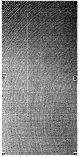
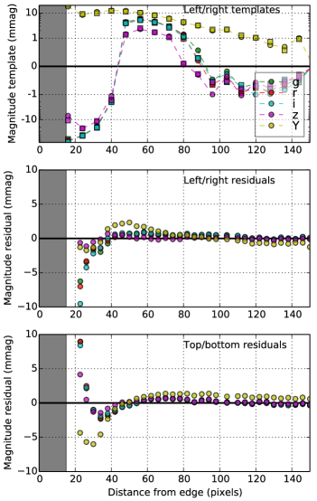
Figure 1: At left is a representative dome flat (CCD N12, $i$-band). Visible behavior is dominated by concentric “tree rings,” a brightening at the edges of the device, and 6 spots where there are spacers between the CCD and its carrier. All of these features are primarily pixel-area variations, not QE variations. We model the photometric effect of the edges and rings, and flag the spots as regions of less-reliable photometry. The grayscale spans a contrast of 5%. At right top are empirical models of the photometric errors induced by the edge effect along the long edges, averaged over all CCDs (note the log scale). At middle right, the residual photometric error vs distance from the long edge after the empirical model has been subtracted from the star flat photometry. At bottom right is the error signal along the short (serial-register) edges, which we do not bother to correct. The 15 pixels nearest each edge are masked in processing, and edge effects are reduced to well below 1 mmag at $\geq 40$ pixels from the edge, except in $Y$ band.

For the edge functions, we first include a free Piecewise function of $x$ pixel coordinate, with nodes spaced at $\Delta x=8$ pixels for $16\leq x\leq 144$ and $1905\leq x\leq 2033$. The 15 pixels nearest all device edges are ignored in DECam processing, as the edge distortions are slightly dependent on illumination level and too large for reliable correction to the desired accuracy. This means that 6″ apertures are incomplete for stars centered $<26$ pixels from any edge, and therefore the photometry corrections that we derive from this aperture photometry is decreasingly reliable within this range. During standard DES processing, objects intruding into this region are flagged as having less reliable photometry (Bernstein et al., 2017b; Morganson et al., 2017).

We perform an initial round of $\chi^{2}$ optimization that leaves all of the nodal values as free parameters (30 per CCD), fitting simultaneously to many epochs of star flats to build up stellar samples. After interpolating over indeterminate nodal values caused by column defects on some CCDs, these lookup tables are converted to Template photomaps with fixed shape for further rounds of fitting.

See Plazas et al. (2014) and Bernstein et al. (2017a) for deeper discussions of these device characteristics. Figures 1 demonstrate that residual edge photometric errors after our corrections are well below 1 mmag, except within a $\approx 20$ pixel strip just inside the masked region (i.e. within $\approx 35$ pixels of the edge), and slightly larger in $Y$ band. The only mystery in this process is that the best-fitting scaling for the tree-ring templates are $s\approx 0.9$ rather than the expected $s=1$, i.e. the spurious stellar photometric signature seems slightly smaller than the fluctuations in the dome flats.

3.3.2 Optics/CCD polynomials

The largest difference between the dome flat and the correct response function ${\bf r}$ is due to contamination of the former by stray light, which we expect to vary smoothly across the FOV. We expect other significant contribution to the star flat correction $S(\mbox{${\bf x}$})$ from the color difference between the dome-flat lamps and the reference stellar spectrum, which in turn depends on the spectral response of each CCD. The DECam photometric model incorporates an independent cubic polynomial per CCD to fit these effects.

The top row of Figure 2 displays the best-fit star flat corrections $S(\mbox{${\bf x}$})$ as a function of position across the array in the $grizY$ filters. The dominant feature in the $g$ and $z$ bands is a “doughnut” which is roughly in the position predicted by models of stray light reflections from the CCD and corrector-lens surfaces. The star flat correction to the dome flat is in excess of 50 mmag peak-to-peak, implying that un-focussed photons comprise at least $5\%$ of the dome flat flux in places. No doughnut is visible in $r,i,$ or $Y$ bands. In $r$ and $i$, the star flat correction is $\approx\pm 10$ mmag in a radial gradient that resembles these filters’ color terms. In $Y$ band we see, in addition, steps between CCDs, readily attributed to variation in the red-edge QE of the devices coupled with a color difference between the dome lamps and the stellar reference spectrum.

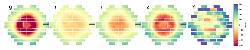
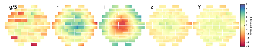
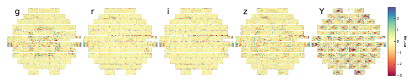
Figure 2: The top and middle rows show the star flat correction $S(\mbox{${\bf x}$})$ and color term $c(\mbox{${\bf x}$})$, respectively, for the DECam $grizY$ bands, derived from fitting to all star flat epochs simultaneously. [Tree ring and edge terms have been suppressed in the top row since they are unresolved at the plotted scale.] These are the corrections that must be applied to stellar photometry of dome-flattened images in order to homogenize the photometric response across the array. The bottom row shows the mean photometric residual, binned by array position, for all unclipped detections in all of the star flat observing sequences. Only a few unmodelled features are visible above 1 mmag level, except in $Y$ band.

3.3.3 Color terms

The color term $c(\mbox{${\bf x}$})$ is also taken to be an independent polynomial per CCD per filter. Linear order suffices to remove any detectable color response patterns. The middle row of Figure 2 shows the best-fit solutions derived by PhotoFit. In $g$ band (and to a lesser extent $Y$ band) we can see the consequences of device-to-device variations in the blue (red) end of the CCD QE spectrum, leading to color terms as large as $\approx 25$ mmag per mag change in $g-i$. Variation from the natural passband is smaller in the other bands, at $\lesssim 5$ mmag/mag. The mild radial gradient in $i$ band is shown by Li et al. (2016) to be consistent with the known radial gradient in the blue-side cutoff wavelength of the filter.

3.3.4 Extinction gradient

Atmospheric extinction will vary across the 1° radius of the DECam FOV. If the zenith angle is $z$, the airmass at the optic axis zenith angle $z_{0}$ is $X=\sec z_{0}$, and the extinction is $kX$ for some constant $k$, then the first-order correction for extinction away from the telescope axis is

$$\Delta m=X\sqrt{X^{2}-1}\,k\,\Delta z.$$ (38)

We take a nominal extinction constant of $k=(0.2,0.1,0.07,0.08,0.07)$ mag per airmass in $(g,r,i,z,Y)$. At the maximum field radius $\Delta z=\pm 1\arcdeg,$ Equation (38) grows to a $\pm 21$ mmag deviation for $X=2$ in $g$ band. The extinction gradient must be corrected, even in the redder bands at more modest airmass, to attain mmag homogeneity. We do so by precomputing a Polynomial photomap for each exposure for the gradient term, which is held constant during fitting. In future DES photometric solutions we could account for temporal variation in the atmospheric extinction constant $k$.

The second derivative of extinction contributes $\Delta m<1$ mmag in peak-to-peak amplitude even at $X=2$ in $g$ band, so we can approximate extinction variation with just the linear term.

3.4 Model residual patterns

The bottom row of Figure 2 shows the residual of the stellar photometry to the PhotoFit solution in each filter, averaged over all star-flat-sequence detections and binned by position in the DECam focal plane. The performance of the model is excellent in $griz$ bands: the RMS of the means in the 34″ square bins is $<1$ mmag and visually consistent with noise, with the exception of a few coherent features at 1–2 mmag level. Residuals are visible at the edges of $g$ and $z$ band doughnuts, indicating sharper edges than our polynomials can capture. There also appear to be features in the east- and west-most CCDs’ response that are higher-order than our cubic.

The $Y$ band shows significantly larger residual variation ($\approx 1$ mmag RMS), which close examination reveals is primarily a repeating pattern on all devices. Figure 3 shows the mean residuals binned by position on the CCD, stacking all devices for all star flat exposures in $Y$ band. Remarkably we see that the star flat detects the presence of metallic structures on the board to which the CCD is mounted. The red edge of the $Y$ band is defined by silicon bandgap energy, and in $Y$ band a significant fraction of stellar photons make it through the CCD to the mounting board, where the reflectivity of the mount will affect QE. A difference between the dome and reference spectra leads to this pattern. It is present at $\ll 1$ mmag in $z$ band and not detected in $g,r,$ or $i.$ We leave this pattern uncorrected since precision $Y$-band photometry is not central to DES science.

The device-stacked residuals in $griz$ bands reveal weak features along the long edges which indicate a break in our assumption that the “glowing edge” is constant for all rows. We leave these patterns uncorrected as well, since they are weak and affect very little of the focal plane.

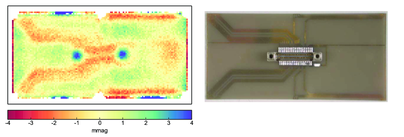
Figure 3: At left: the residual stellar magnitude errors in $Y$ band, after star flat correction, binned by position on the CCD. All CCDs and all star flat epochs are stacked. The $\Omega$ shape follows the traces on the aluminum nitride board to which the devices are mounted, shown at right (courtesy J. Estrada and T. Diehl).

3.5 Error statistics

Our goal is to eliminate any variance in magnitude estimates of stars in excess of that expected from photon shot noise and detector read noise. We define the excess RMS noise $\sigma_{\rm sys}$ as

$$\sigma^{2}_{\rm sys} \equiv\left\langle\Delta m_{i}^{2}-\sigma^{2}_{{\rm stat},i}\right\rangle,$$ (39)

$$\Delta m_{i} \equiv\frac{m_{i}-\bar{m}}{\sqrt{1-w_{i}/\sum w_{j}}},$$ (40)

$$w_{i} \equiv\sigma_{{\rm stat},i}^{-2},$$ (41)

$$\bar{m} \equiv\frac{\sum w_{j}m_{j}}{\sum w_{j}}.$$ (42)

This $\sigma_{\rm sys}$ is distinct from the value used to set an error floor in Equation (18), though the value measured here is a good choice for setting the error floor. The $\sum w_{j}$ terms are over all measures of the same star. Note that $\Delta m_{i}$ is normalized such that the expectation of $\sigma^{2}_{\rm sys}$ is zero if each measurement $m_{i}$ has variance equal to its expected statistical noise $\sigma_{{\rm stat},i}$ and all measurements have independent errors. SExtractor provides an estimate of $\sigma_{{\rm stat},i}$ expected from the photon shot noise and read noise within the stellar aperture.

The left panel of Figure 4 plots the excess RMS noise vs stellar instrumental magnitude for the 20131115 star flat data. The data are consistent with the dotted curves for the model

$$\sigma^{2}_{\rm sys}=\sigma^{2}_{m}+\left(\frac{2.5}{\log 10}\right)^{2}\left(\frac{\sigma_{f}}{f}\right)^{2}.$$ (43)

The free parameters of this model are: $\sigma_{m}$, an error that is fixed in magnitudes and hence represents a multiplicative error in flux as would be expected from flat-fielding imperfections; and $\sigma_{f}$, an error that is fixed in flux units.

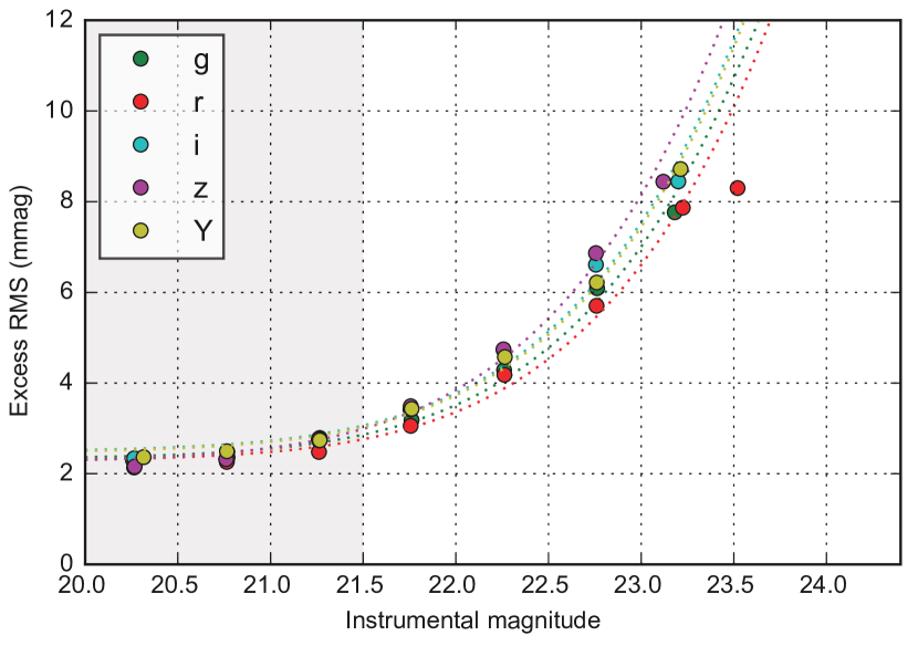
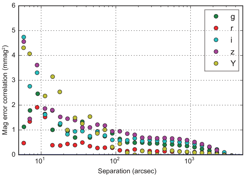
Figure 4: Left: the RMS excess magnitude noise, defined by Equation (39), is plotted against instrumental magnitude for exposures from the 20131115 star flat sequence for each filter. The dotted lines show fits to the model of Equation (43). There is a 2–3 mmag floor on the magnitude errors above statistical noise. Further statistical analyses make use of stars in the shade range of magnitudes. At right is the 2-point correlation function of magnitude residuals for the same data. In $griz$ bands, any photometric errors correlated at separations $\geq 20\arcsec$ are $<1$ mmag.

We believe that the non-zero fixed-flux error $\sigma_{f},$ is attributable to noise in the estimation of the sky level due to shot noise in the annulus used for local sky determination. SExtractor does not include such noise in its error estimation, and we find that propagating the expected sky-annulus mean error into flux measures in our large (6″) apertures yields roughly the right level of $\sigma_{f}$. Reducing the size of the photometric aperture from 6″ to 4″ diameter reduces $\sigma_{f}$ by very close to the ratio $(4/6)^{2}$ of aperture area, supporting this hypothesis. Henceforth we will concentrate analysis of the residual errors on stars with instrumental magnitude $20<m_{i}<21.5$, corresponding to $>10^{4}\,e$/s flux, where the effects of $\sigma_{f}$ are subdominant to the calibration errors $\sigma_{m}$ that are our primary interest.

The derived values of $\sigma_{m}$ are in the range 2–3 mmag for most of the star-flat exposures. The star flat solutions for a given night homogenize the array calibration to 2–3 mmag RMS. The level of excess variance does change over time—some nights or exposures are worse, as we will investigate below.

More indicative of photometric calibration errors is the 2-point angular correlation function (2PCF) $\xi_{m}(\theta)$ of the magnitude residuals $\Delta m_{i}$. We consider only measurement pairs within the same exposure. Shot noise within the stellar aperture will not contribute to the 2PCF, nor will stellar variability, and shot noise within the sky annuli will not contribute beyond the $\approx 20\arcsec$ diameter of the SExtractor local sky annuli. As seen the right panel of Figure 4, the 2PCF amplitude at $\theta>20\arcsec$ separation is typically below 1 mmag² in $griz$ bands. The slightly higher level in $Y$ band is likely due to the uncorrected static pattern detected in Figure 3. The level of correlated noise at $\theta>20\arcsec$ does exceed 1 mmag in some exposures or consistently on some nights, which will be characterized in Section 4.

We conclude that most of the 2–3 mmag excess calibration noise arises from effects with short coherence length. Stellar variability would produce such a signature, but each filter’s star flats span $<30$ minutes time so this is likely unimportant for this analysis. Aside from the tree rings and glowing edges, our star flat models do not attempt to correct small-scale error in the dome flats. A close look at the dome flats reveals pixel-to-pixel variations that repeat from band to band. These are probably pixel-area variations from imperfections in lithography of the CCD gate structure. If we ascribe all the small-scale variation in the dome flats to pixel-area rather than QE changes, we estimate that in seeing of 1″ FWHM, these flat-field errors induce $\sigma_{m}\approx 1.2$ mmag. In worse seeing, $\sigma_{m}$ decreases as the signal spreads over more pixels and averages down the gate errors. These single-pixel-scale errors are essentially impossible to characterize with on-sky measurements. Future experiments, such as LSST, would benefit from laboratory characterization of lithographic errors if it is desired to reduce excess RMS to $<1$ mmag. We note, though, that for DES measurements such as galaxy clustering, bias is induced only by calibration errors that correlate between targets, and we have demonstrated that these can be reduced to $\approx 1$ mmag for time scales $<1$ hour.

4 Short-term stability

For each star flat epoch, we have fit a fixed solution to all 22 exposures in a given filter. For the analyses in this section, the only additional degree of freedom in an individual exposure’s solution is an overall Constant photomap to allow for zeropoint variation. Recall that we also have a term per exposure for extinction gradient, but this is held fixed to an a priori model. We now look for patterns in the deviations of individual exposures’ photometry from the night’s solution, i.e. is there detectable variation in photometric response pattern within the $\approx 25$ min it takes to expose a given filter?

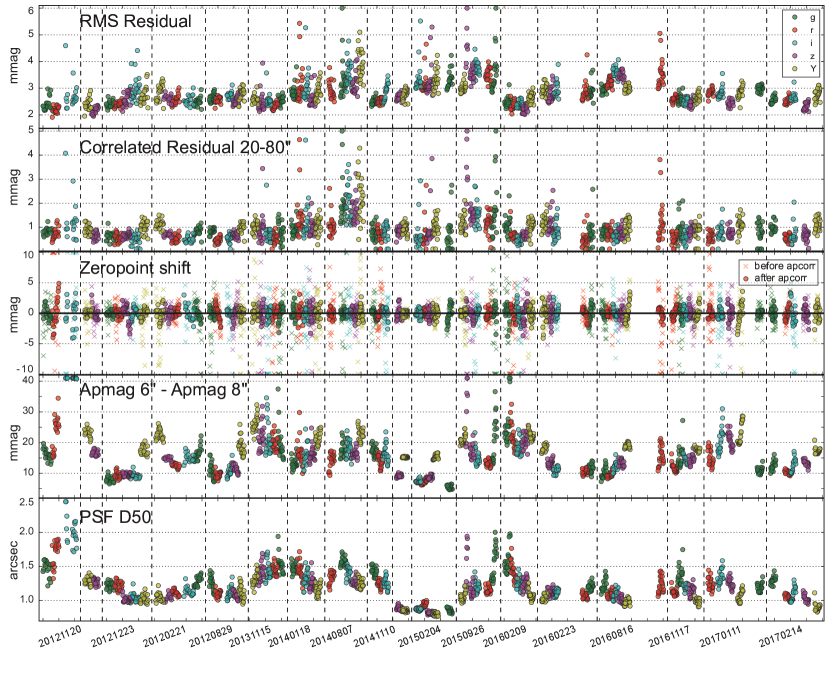
Figure 5: Each panel shows a photometry-related variable for each of the $\sim 1800$ exposures taken during the 16 cloudless star-flat observing epochs. The tick marks on the horizontal axis mark 1-hour intervals, but the vertical dashed lines represent breaks of days to months. For this plot, each star flat epoch has its own photometric solution. The top row plots the RMS photometric noise above the expected shot noise for stars with instrumental magnitude $20<m_{\rm inst}<21.5,$ for which the errors from sky-level determination are usually negligible. Most nights this is 2–3 mmag, but some nights and individual exposures are worse. The second row plots the RMS amplitude of correlated magnitude errors, $\sqrt{\xi_{m}(20\arcsec<\theta<80\arcsec)},$ which is seen to be $\approx 1$ mmag in $griz$, again with a few nights and a few stray exposures of higher level. The third row plots the deviation of the exposure zeropoint shift from the atmospheric secant law for that night. The crosses give the initial values, which are 2–5 mmag RMS, but when the aperture correction of Section 4.3 is applied, the RMS zeropoint variation is reduced to $\approx 1$ mmag. The fourth row shows the aperture correction proxy $A_{t}$, the difference between 8″ and 6″ aperture magnitudes. The fifth row plots the half-light diameter $D_{50}$ of the PSF, which is seen to be less than fully predictive of $A_{t}$ or the zeropoint shifts.

Figures 5 plot the primary diagnostics for unmodelled time variation in photometric response. Of most interest is the second row: we plot the amplitude of coherent magnitude residuals $\sqrt{\xi_{m}(\theta)}$ using a broad bin $20\arcsec<\theta<80\arcsec$ (see Figure 4). Usually $\sqrt{\xi_{m}(\theta)}\leq 1$ mmag (except in $Y$ band)—excursions above 2 mmag indicate the presence of changes in the response pattern. Additional evidence of varying instrument response is given by elevated RMS residual of bright stars, plotted in the top row, although keep in mind that the RMS can also be inflated by errors in sky background determination, which are not of interest in this paper.

4.1 Freaks

There are occasional isolated instances of higher photometric residuals in a single exposure, for example #275794 taken during the 20131115 $i$-band star flat sequence. The top row of Figure 6 plots the photometric residuals to the static model observed on a series of 5 consecutive exposures. Exposure 275794 exhibits large coherent residuals of $\pm 10$ mmag, while exposures taken just 1 minute earlier or later have the usual $\approx 1$ mmag RMS residual.

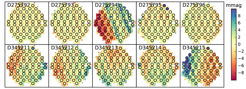
Figure 6: The background of each panel plots the spatially binned residual photometric errors of bright stars in a single exposure, after application of the static starflat and color corrections $S(\mbox{${\bf x}$})$ and $c(\mbox{${\bf x}$})$. The colors of the overplotted circles encode $2\times$ the variation of the aperture correction proxy $A_{ti}$ (equation 37) across the FOV. It might be difficult to notice that the colors inside the circles are different from the color just outside the circles, which tells us that the variation in $A_{ti}$ is a very accurate predictor of the spatial pattern of photometric errors. The top row shows a series of star flat exposures at 1 minute interval containing one freak excursion. The lower row shows a sequence of exposures during a period of very unstable seeing. In all cases the photometric inhomogeneity is clearly attributable to variations in the fraction of flux falling outside the nominal 6″ photometric aperture.

We find strong evidence that these residuals are due to spatial fluctuations in the aperture correction rather than in the transparency of the atmosphere, as follows. Define $A_{ti}$ to be the median differences between 8″ and 6″ aperture magnitudes of bright stars on CCD $i$ in exposure $t$, as per Equation (37). The color of each circle overplotted in Figure 6 indicates $2(A_{ti}-\langle A_{ti}\rangle)$ for each of the 60 CCDs in use for these exposures. This scaling of the aperture-correction proxy $A_{ti}$ is seen to be a near-perfect match to the pattern of photometric residuals across the FOV for this exposure. From this we conclude that (a) the excess correlated photometric errors in this exposure are caused by variations in aperture correction across the FOV, and (b) the statistic $A_{ti}$ is a good tracer of such variations.

What caused this freak exposure on an otherwise well-behaved, cloudless night? The streaky appearance of the residuals is likely the result of some disturbance being blown across the field of view during the exposure. We do not have any well-supported theories for what kind of disturbance would cause a localized increase in the PSF wing strength. The number of outlier points in the second row of Figure 5 gives some indication that $O(1\%)$ of exposures have freak disturbances, in addition to there being some nights with consistently high correlated residuals. One possibility, as yet unverified, is that these are associated with elevated levels of scattering or turbulence in airplane contrails.

4.2 Noisy nights

On some nights $\xi_{m}$ is consistently or frequently well above the typical 1 mmag² level, i.e. on the nights 20140807 and 20150926. The lower panel of Figure 6 shows the magnitude residuals for a series of 5 consecutive $z$-band exposures on the latter night, during which the seeing half-light diameter underwent a rapid excursion from 1$\farcs$3 to 2$\farcs$0 and back (see bottom row of Figure 5). The overplotted circles in Figure 6 once again indicates that the photometric errors are closely tracked by variations in the aperture correction proxy $A_{t}$ across the focal plane.

Indeed it is found that nearly every star-flat exposure $t$ with high photometric residual $\sqrt{\xi_{m}}$ is accompanied by higher-than average dispersion of the $A_{ti}$ across the focal plane.

4.3 Zeropoint stability

A basic question of critical importance to ground-based photometric survey calibration is: just how stable is the atmospheric transmission on a given night, apart from expected scaling with $\sec z$? We answer this question by calculating the deviation between each exposure’s zeropoint and the best-fitting secant law, as in the numerator of Equation (20). We adopt $\sigma_{n}=0.5$ mmag in our atmospheric prior to give the $\chi^{2}$ minimization strong incentive to reduce the zeropoint residual to mmag level.

Table 3: Zeropoint variation per filter

Band	$g$	$r$	$i$	$z$	$Y$
RMS variation before aperture correction (mmag)	2.6	3.1	4.5	1.9	2.9
RMS variation after aperture correction (mmag)	0.9	0.7	0.8	1.1	1.0
Nominal apcorr coefficient $k_{n3}$	1.6	1.9	1.9	1.9	2.2

The crosses in the third row of Figure 5 plots these residuals for each star flat exposure before we introduce any aperture corrections, i.e. we set the aperture correction coefficient $k_{n3}=0$ in Equation (19). The RMS values in each filter, shown in the first row of Table 3, are 2–5 mmag. There is substantial variation in RMS from night to night, and deviations $>10$ mmag in individual exposures are common.

The temporal zeropoint jitter is highly correlated with estimators of the fraction of light falling outside the photometric aperture. The fourth and fifth rows of Figure 5 show two variables we might expect to correlate with the aperture correction, namely the half-light diameter of the PSF (bottom row) and the $A_{t}$ defined in Equation (37) as the fraction of extra light found in extending the aperture from 6″ to 8″. Both quantities are the median of all bright stars in the field. The latter variable is found to correlate much better with the zeropoint jitter. $A_{t}$ does not measure the aperture correction to infinity, but it is sensible to think that the aperture correction to 8″ would correlate with the correction to infinity, so we introduce the term $k_{n3}\times A_{t}$ into the zeropoint model as per Equation (20) essentially as an adjustment to each exposure’s zeropoint. Leaving $k_{n3}$ as a free parameter on each night reduces the zeropoint jitter to $\leq 1$ mmag RMS ($z$ band is slightly higher, perhaps due to some variability in water vapor absorption).

We find that setting $k_{n3}$ to a nominal value in each filter yields zeropoint jitter indistinguishable from having a free value for each night. The nominal $k_{n3}$ values and the resultant RMS values per filter are in Table 3. The circles in the 3rd row of Figure 5 show the truly impressive stability in atmospheric transmission obtained after making the zeropoint correction.

In summary, we find that all of the deviations above $\approx 1$ mmag RMS from a static response function plus secant airmass law on short timescales are plausibly attributable to spatial/temporal variations in aperture corrections. The $A_{t}$ statistic measured from bright stars is an accurate predictor of these aperture corrections, so on a typical half-hour stretch of clear-sky observations we can homogenize the exposure zeropoints to $\approx 1$ mmag, and if we have sufficient stellar data in an exposure to map out variation of $A_{t}$ across the FOV, we could reduce any intra-exposure inhomogeneity to similar level.

5 Long-term stability

To investigate the stability of the reference response $\mbox{${\bf r}$}(t)$ over months to years, we fit the entire multi-year ensemble of star flat data to a common instrument model and examine the mean residuals to this model in each epoch (recall they have all be flattened with a common dome flat too). We observe changes of several mmag between star flat epochs, smoothly varying across the focal plane, and very similar in all filters. This “gray” term might arise from accumulation of dust or contaminants on one of the lenses (or the detectors).

The $Y$ band exhibits additional shifts in the response of specific CCDs. After cycling the camera to room temperature, the strength of some thermal contacts change slightly and the equilibrium temperatures of the devices change slightly. It is thought that these temperature shifts will then change the silicon optical depth near the band gap and slightly alter the $Y$-band response.

Whenever we jointly fit data from multiple observing nights, we allow a constant Color photomap for each exposure, as it is expected that variations in atmospheric constituents will change the color response of the system by up to several mmag (Li et al., 2016; Burke et al., 2017).

5.1 Test of gray drift model

To test the hypothesis that long-term changes in instrument response are due to low-order gray absorption plus CCD-specific changes in $Y$-band response, we derive a new global response model as follows:

1. Run PhotoFit jointly on the $i$ and $z$-band exposures from all star flat epochs, adding an additional 4th-order Polynomial photomap to the model. Each epoch (except one reference epoch) is allowed an independent gray drift term that is common to both filters.

2. Run PhotoFit on the $g$ filter’s data, augmenting the model with a drift term for each epoch whose parameters are held fixed to the values derived in step (1). Repeat for $r,$ $i,$ and $z$ bands.

3. Run PhotoFit on the $Y$ data, including the fixed drift terms plus an additional free Constant for each CCD (except one) in each epoch, to track the temperature changes.

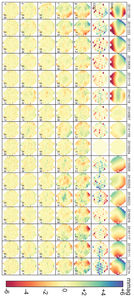
Figure 7: The top row shows the 4th-order polynomial “drift” for each epoch that best brings its $iz$ photometric response into agreement with epoch 20150204. The second row shows the shifts of CCD response that are further applied to homogenize the $Y$-band photometry. Further rows show the mean photometric error in 1024-pixel bins at each epoch and filter, to a model including the gray polynomial drift terms (and CCD shifts, for $Y$ band). The number in lower-right of each panel is the RMS of the binned residuals (in mmag). A common polynomial in all bands captures the epoch-to-epoch changes in response to $<1$ mmag RMS in the $iz$ bands, but an unmodelled bluer component is apparent in the $g$-band residuals with a weaker $r$-band signature.

Figure 7 plots the results of including the drift terms in a fit to more than 4 years’ star flat data. The top row shows the derived gray polynomial terms, which exhibit amplitude up to $\pm 6$ mmag and RMS up to 2.5 mmag. The second row plots the $Y$-band CCD shift terms per epoch, which are as large $\pm 12$ mmag for the worst devices in the worst epochs.

The remaining rows plot the mean photometric residual to the gray drift model across the focal plane for each filter and each epoch. The RMS residual signal is below 1 mmag RMS (some of which is measurement noise and stellar variability) at all times in $izY$ bands. The gray model is seen to be not quite sufficient: there appears to be an additional blue drift component, present in $g$ band with a fainter version in $r$ band. This pushes the RMS residual to the gray model up to 2 mmag in the worst $g$-band epochs. We note that even if this $g$-band deviation were not corrected, the 2 mmag RMS photometric variation would be well below DES requirements and far better than any previous survey’s photometric calibration accuracy.

5.2 Time history of drifts

The star flat sequences are taken too infrequently to resolve the time scale for instrumental response changes. DES observes its supernova fields roughly once per week during the observing seasons. The SN exposures are taken with minimal dithering, so that the same stars are on a given CCD in every exposure. This makes the data useless for determining the spatial structure of the response function $\mbox{${\bf r}$}(t)$, but valuable for examination of its temporal structure at finer resolution. We will use the $z$-band data from field SN-C3, for which an observing sequence comprises $11\times 330$ s exposures. Roughly 2000 stars are available at $S/N\gtrsim 30$, are not saturated, and have well-determined $g-i$ colors falling within the calibratable range. Through October 2016, there are 72 nights of SN-C3 $z$-band observations for which there is no evidence of clouds and the mean seeing half-light diameter is $<1\farcs 6.$

Images for these exposures were processed using a fixed dome flat for all 4 years’ data, and the PhotoFit assumed a fixed instrumental response model, with parameters fixed to those determined from the star flat observations. Each SN-C3 exposure is given a free zeropoint and color term, and an extinction gradient correction determined a priori. The atmospheric prior for each night has fixed values $k_{n1}=0.08$ for the airmass term and $k_{n3}=1.5$ for the aperture correction coefficient. After the fit we calculate the residual deviation of the stellar instrumental magnitudes from the PhotoFit model. Our analysis tracks variation of the camera response using the median residual deviations $\Delta m_{ni}$ of the stellar detections in CCD $i$ on night $n.$

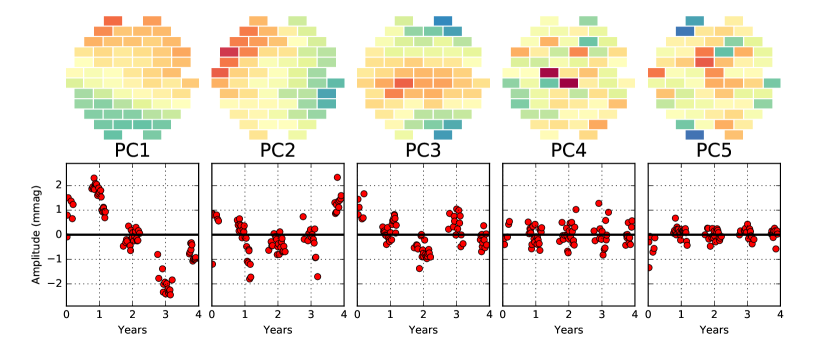
Figure 8: First 5 principal components of variation in the response of DECam CCDs to the stars in the SNC3 field. The top row shows the pattern of principal components—the first three are smooth functions of array coordinates. The bottom row plots the coefficient of each PC for each night of observations; the PCs are normalized such that these coefficients are in units of the RMS fluctuation across the focal plane contributed by the PC. The first three are seen to vary smoothly with time over the first 4 years of the survey. The fourth PC does not (but does correlate with seeing). The fourth and higher PCs contribute less than 1 mmag RMS photometric error.

Changes in the photometric residual pattern are observed to be smooth in both time and in position on the array. To quantify this, we identify the principal components (PCs) of the $\Delta m_{ni}$ matrix. The five PCs contributing the most variance are plotted in the top row of Figure 8. The first three of these are seen to vary smoothly across the focal plane and are clearly related to the patterns seen in the drift solutions for the star flats (top row of Figure 7). The lower row of Figure 8 plots the temporal behavior of these PCs: their amplitudes are seen to change slowly over the course of each observing season. PC1 is a roughly north-south gradient that changes by several mmag across the FOV over the lifetime of the camera.

PCs beyond the third exhibit little spatial coherence and lack overall temporal trends. We find that PC4 correlates with the seeing, and suspect that it maps small errors in our nonlinearity corrections for the amplifiers. This effect is small, producing, $\ll 1$ mmag RMS photometric variation for bright stars. Further PCs are even less significant.

We conclude that the camera’s photometric response changes by up to $\pm 7$ mmag on scales of months. Any changes on scales of days are well below 1 mmag. The response variations are low-order functions of focal-plane position and hence likely to be caused by slow accumulations of dust or contaminants on the optical surfaces.

The few-mmag shifts in CCD response seen in $Y$ band are thought to be an exception, since the changes in CCD operating temperatures occur when the focal plane is cycled to room temperature and back, a few times per year. The SN fields are not observed in $Y$ band so we cannot verify this hypothesis directly.

6 Implications

The photometric characterization of $\approx 1800$ specialized DECam images of rich stellar fields yields a response model that is accurate at mmag level across the focal plane and across 4 years of DECam operations. The ability to homogenize response of the instrument and (on cloudless nights) the atmosphere to this level encourages future attempts to calibrate the entire DES survey at accuracy significantly better than the $\approx 7$ mmag RMS repeatability achieved for DES by Burke et al. (2017) and for PS1/SDSS by Finkbeiner et al. (2016). A successful few-mmag calibration model for DECam requires these key elements:

• Stable camera and electronics, such that the response of the system on a clear night stays constant over a period longer than the time required to characterize it.

• Combination of internal-consistency constraints (“ubercal”) with prior assumptions on atmospheric and instrumental stability to remove large-scale degeneracies.

• An instrumental reference response map $\mbox{${\bf r}$}(t)$ that is free of the spurious signals present in dome flats due to stray light, pixel-scale variations, and spectral mismatches between the flat-field illumination and stellar spectra.

• Accommodation of spatial and temporal variations of the spectral response $\mbox{${\bf r}$}(\lambda,t)$ from the reference “natural” passband of the instrument, which can be empirically determined in the form of a color correction $\mbox{${\bf c}$}(t)$.

• Use of a measurable aperture correction proxy, such as the fraction of the PSF found in a large but finite annulus, to compensate for temporal variation in atmospheric scattering of light out of the photometric aperture.

• Allowance for slow (weeks to months), low-order drifts in the spatial structure of $\mbox{${\bf r}$}(t)$. These drifts are close to, but not quite, wavelength independent. The camera response is much more stable than the dome screen illumination.

• Recognition of the contribution of sky-estimation errors to the uncertainty budget for photometry.

• Achieving mmag repeatability in $Y$ band would additionally require a spatial correction for flat-field errors related to the mounting structure of the CCDs, and a temporal correction for shifts in CCD operating temperatures.

After implementing these techniques, we find that the $griz$ stellar photometry of the star-flat exposures is highly repeatable. In most exposures on most nights, the key quantifications of this are:

• The level of correlated photometric errors, as measured by the correlation function $\xi_{m}(\theta)$ of stellar magnitude residuals on scales $20\arcsec<\theta<80\arcsec,$ is 1 mmag² or lower.

• The RMS magnitude errors, in excess of those expected from shot noise and read noise, are 2–3 mmag. Effects that can be making this (zero-lag) RMS larger than the $\approx 1$ mmag of correlated error include: sky estimation errors; small-scale variations in pixel size due to lithography “noise”; limitations of the approximation of bandpass variation by a linear color term; or, on longer time scales, stellar variability.

• After application of the aperture correction proxy terms, the RMS deviation of exposure zeropoints from a simple atmospheric secant law is $\approx 1$ mmag.

• A wavelength-independent 4th-order polynomial function of focal plane coordinates captures temporal changes in array response to $<1$ mmag accuracy in $i$ and $z$ bands, with up to 2 mmag RMS variation in $g$ and $r$ bands. The blue component of the response drift could also be modeled to improve $g$ and $r$ accuracy.

DECam is remarkably stable and well-behaved. For example, no changes in amplifier gain have been detected (with the exception of a 3% shift in the gain of one amplifier of CCD S30 when it came back to life after being non-functional for 3 years). The spectral response shows no evidence of change over time aside from that expected from variability of atmospheric constituents. The spatial response does change over time by up to $\pm 7$ mmag (Figure 7, top row). Although we do not know the physical origin of this drift, it is gradual and hence calibratable.

The transmission of the atmosphere on cloudless nights at airmass $X<2$ is found to be described by a secant law to 1 part per thousand on most nights. Instances where correlated photometric errors rise perceptibly above 1 mmag are all found to be correlated with the aperture-correction proxy $A_{t}$, so we can conclude that the primary photometric impact of atmospheric perturbations is via scattering of light outside our 6″ aperture. The aperture corrections can change rapidly and unpredictably by up to $\approx 10$ mmag, and some nights show elevated variability. Fortunately the 6″–8″ annular flux fraction ($A_{t}$) is directly measurable from the images and can be used to correct these temporal, and perhaps spatial, variations in aperture correction.

Our star-flat observations span only 25 minutes of clock time in each filter. Further investigation will be necessary to characterize the amount of variation in atmospheric transmission that occurs over the course of an entire evening. This will be an important aspect of extending our achieved level of accuracy to a global photometric solution for DES. The DES observing strategy is well-suited to the task of global homogenization of photometry: each spot on the sky will be observed in a given filter 8–10 times, on different parts of the array, on different nights in different years, averaging down any remnant spatial or temporal errors in photometric calibration. Exposures are heavily interlaced for strong internal constraints, and widely separated areas of sky are observed on each cloudless night to generate constraints on large-scale modes of the calibration solution.

These DECam results should be indicative of the techniques and potential for other ground-based surveys to move from $\approx 10$ mmag photometric calibration toward the $\approx 1$ mmag regime. In particular, the Large Synoptic Survey Telescope (LSST) will be able to employ all of the methods that succeed with DECam, with vastly more exposures per sky location and stellar detections per exposure, albeit with the substantial additional complication of calibrating dependence upon the varying camera/instrument rotation angle required for LSST’s alt-az mount. Our study emphasizes the utility of periodic “star flat” observing sequences, with a range of dither steps on a single field, and also the calibration utility of more frequent observations of fixed pointings such as the supernova search areas. Attempts to push photometric calibration of ground-based visible imaging to $<1$ mmag accuracy will need to address several new problems, including: characterization of pixel-to-pixel lithographic variation; the inadequacy of simple linear color corrections in describing the departures of system throughput from the natural bandpass; inaccuracies in our aperture-correction proxy; and, ultimately, scintillation. Specialized observing procedures, such as defocussing, have been used to overcome these barriers, but may not be practical for general-purpose survey observations. But averaging of many repeat observations, with dithered exposures, will serve to beat down most of these potential sub-mmag systematic errors.

References

- Antilogus et al. (2014) Antilogus, P., Astier, P., Doherty, P., Guyonnet, A., & Regnault, N. 2014, Journal of Instrumentation, 9, C03048
- Bernstein et al. (2017a) Bernstein, G. M., Armstrong, R., Plazas, A. A., et al. 2017, PASP, 129, 074503
- Bernstein et al. (2017b) Bernstein, G. et al., 2017b, arxiv:1706.09928
- Bertin (2006) Bertin, E. 2006, Astronomical Data Analysis Software and Systems XV, 351, 112
- Bertin & Arnouts (1996) Bertin, E., & Arnouts, S. 1996, A&AS, 117, 393
- Betoule et al. (2014) Betoule, M., Kessler, R., Guy, J., et al. 2014, A&A, 568, A22
- Burke et al. (2014) Burke, D. L. et al. (2014), AJ, 147, 19
- Burke et al. (2017) Burke, E. et al. (2017), arxiv:1706.01542
- Drlica-Wagner et al. (2017) Drlica-Wagner, A., Sevilla-Noarbe, I., Rykoff, E. S., et al. 2017, arXiv:1708.01531
- Estrada et al. (2010) Estrada, J., Alvarez, R., Abbott, T., et al. 2010, Proc. SPIE, 7735, 77351R
- Finkbeiner et al. (2016) Finkbeiner, D. P., Schlafly, E. F., Schlegel, D. J., et al. 2016, ApJ, 822, 66
- Flaugher et al. (2015) Flaugher, B., Diehl, H. T., Honscheid, K., et al. 2015, AJ, 150, 150
- Henden & Munari (2014) Henden, A., & Munari, U. 2014, Contributions of the Astronomical Observatory Skalnate Pleso, 43, 518
- Li et al. (2016) Li, T. S., DePoy, D. L., Marshall, J. L., et al. 2016, AJ, 151, 157
- Plazas et al. (2014) Plazas, A. A., Bernstein, G. M., & Sheldon, E. S. 2014, PASP, 126, 750
- Gruen et al. (2015) Gruen, D., Bernstein, G. M., Jarvis, M., et al. 2015, Journal of Instrumentation, 10, C05032
- Gunn & Westphal (1981) Gunn, J. E., & Westphal, J. A. 1981, Proc. SPIE, 290, 16
- Jacoby et al. (1998) Jacoby, G. H., Liang, M., Vaughnn, D., Reed, R., & Armandroff, T. 1998, Proc. SPIE, 3355, 721
- Manfroid (1995) Manfroid, J. 1995, A&AS, 113, 587
- McLeod et al. (1995) McLeod, B. A., Bernstein, G. M., Rieke, M. J., Tollestrup, E. V., & Fazio, G. G. 1995, ApJS, 96, 117
- Morganson et al. (2017) Morganson, E. et al. (2017), in preparation
- Padmanabhan et al. (2008) Padmanabhan, N., Schlegel, D. J., Finkbeiner, D. P., et al. 2008, ApJ, 674, 1217-1233
- Press et al. (2003) Press, W. H., Teukolsky, S. A., Vetterling, W. T., & Flannery, B. P. 2003, Numerical Recipes in C++, Cambridge University Press
- Reil et al. (2014) Reil, K., Lewis, P., Schindler, R., & Zhang, Z. 2014, Proc. SPIE, 9149, 91490U
- Skrutskie et al. (2006) Skrutskie, M. F., Cutri, R. M., Stiening, R., et al. 2006, AJ, 131, 1163
- Tyson (1986) Tyson, J. A. 1986, Journal of the Optical Society of America A, 3, 2131