Passive scalar transport in rotating turbulent channel flow

Abstract

Passive scalar transport in turbulent channel flow subject to spanwise system rotation is studied by direct numerical simulations. The Reynolds number $Re=U_{b}h/\nu$ is fixed at $20\,000$ and the rotation number $Ro=2\Omega h/U_{b}$ is varied from 0 to 1.2, where $U_{b}$ is the bulk mean velocity, $h$ the half channel gap width and $\Omega$ the rotation rate. The scalar value is constant but different at the two walls, leading to steady scalar transport across the channel. The rotation causes an unstable channel side with relatively strong turbulence and turbulent scalar transport, and a stable channel side with relatively weak turbulence or laminar-like flow, weak turbulent scalar transport but large scalar fluctuations and steep mean scalar gradients. The distinct turbulent-laminar patterns observed at certain $Ro$ on the stable channel side induce similar patterns in the scalar gradient field. The main conclusions of the study are that rotation reduces the similarity between the scalar and velocity field and that the Reynolds analogy for scalar-momentum transport does not hold for rotating turbulent channel flow. This is shown by a reduced correlation between velocity and scalar fluctuations, and a strongly reduced turbulent Prandtl number of less than 0.2 on the unstable channel side away from the wall at higher $Ro$. On the unstable channel side, scalar scales become larger than turbulence scales according to spectra and the turbulent scalar flux vector becomes more aligned with the mean scalar gradient owing to rotation. Budgets in the governing equations of the scalar energy and scalar fluxes are presented and discussed as well as other statistics relevant for turbulence modelling.

I 1. Introduction

In this paper, I present a numerical study of passive scalar transport in turbulent channel flow subject to spanwise system rotation. A passive scalar, a scalar that does not influence the flow, can represent e.g. a contaminant or small temperature variation. The present investigation is therefore connected to heat and mass transfer in rotating flows. Examples of these can be found in many industrial apparatus such as turbo machinery, separators and chemical reactors.

Brethouwer (2005) and Kassinos et al. (2007) investigated passive scalar transport in homogeneous turbulent shear flow subject to rotation about an axis normal to the mean shear plane by direct numerical simulations (DNS). They found that rotation has a large impact on the scalar fluctuation intensity and direction of turbulent scalar transport. With a transverse mean scalar gradient, scalar transport is predominantly in the streamwise direction if the flow is non-rotating, but if the system rotation exactly counteracts the rotation by the mean shear the scalar transport is nearly aligned with the mean scalar gradient. Brethouwer (2005) observed that rotation can strongly reduce the turbulent Prandtl number. Many of these rotation effects are also shown by rapid distortion theory (Brethouwer 2005).

A generic case to investigate the influence of system rotation on mass or heat transfer in wall flows is turbulent plane channel flow including a passive scalar subject to spanwise system rotation. The effect of spanwise rotation on turbulent channel flow has already been thoroughly investigated numerically (see e.g. Kristoffersen & Andersson 1993, Grundestam et al. 2008, Xia et al. 2016) and experimentally (see e.g. Johnston et al. 1972). Most of the numerical studies are limited to $Re_{\tau}=u_{\tau}h/\nu\leq 194$, where $u_{\tau}$ is the friction velocity, $h$ the half channel gap width, $\nu$ the viscosity, but recently I have extended the study of spanwise rotating channel flow to $Re=U_{b}h/\nu=31\,600$ and a wide range of rotation numbers $Ro=2\Omega h/U_{b}$ (Brethouwer 2017). Here, $U_{b}$ is the bulk mean velocity and $\Omega$ the system rotation rate. The main conclusions of these studies can be summarized as follows. Turbulence and especially the wall-normal velocity fluctuations are augmented on the channel side were the system rotation is anti-cyclonic, i.e. in the direction opposite to the rotation induced by the mean shear, while they are damped on the channel side were the rotation is cyclonic at moderate $Ro$ (Xia et al. 2016). These channel sides are from now on called the unstable and stable sides, respectively. Large streamwise roll cells, sometimes called Taylor-Görtler vortices, are observed on the unstable channel sides at low to moderate $Ro$ (Liu & Lu 2007, Dai et al. 2016, Brethouwer 2017). The flow on the stable side relaminarizes partly or fully at moderate $Ro$ whereas in the limit of very high $Ro$ the whole channel relaminarizes (Grundestam et al. 2008, Wallin et al. 2013, Brethouwer 2017). A key feature of spanwise rotating channel flow is the development of linear part in the mean streamwise velocity profile on the unstable side where the absolute mean vorticity is nearly zero (Grundestam et al. 2008, Xia et al. 2016). Another remarkable feature is the occurrence of a linear instability in a range of $Re$ and $Ro$, which leads to recurring strong bursts of turbulence on the stable channel side (Brethouwer et al. 2014, Brethouwer 2016).

Passive scalar transport in non-rotating turbulent channel flow has been investigated extensively as well, see e.g. the DNS studies by Kawamura et al. (1998, 1999) and Johansson & Wikström (1999). The velocity and scalar fields show a quite high degree of similarity in several aspects, especially near the wall (Abe & Antonia 2009, Antonia et al. 2009, Dharmarathne et al. 2016). Pirozzoli et al. (2016) carried out DNS of passive scalar transport in turbulent channel flow for $Re_{\tau}$ up to 4088 and Prandtl number $Pr=\nu/\alpha$ between 0.2 and 1, where $\alpha$ is the scalar diffusivity. They observed that the mean scalar profiles follow a logarithmic law and that large-scale structures are present in the scalar field in the outer layer. The turbulent Prandtl number was found to be close to 0.85 in a large part of the channel, suggesting that the Reynolds analogy for scalar-momentum transfer is valid in a non-rotating turbulent channel flow.

Scalar transport in rotating channel flow has been much less examined. Matsubara & Alfredsson (1996) have experimentally investigated the momentum and heat transfer in a laminar rotating channel flow. They found that streamwise roll cells, present at higher rotation rates, have a profound effect on heat transfer, and concluded that the Reynolds analogy is not valid since the Nusselt number changes but not the skin friction under the influence of rotation. Nagano & Hattori (2003) and Liu & Lu (2007) carried out DNS of passive scalar transport in spanwise rotating turbulent channel flow at $Re_{\tau}=150$ and 194, respectively, for $Ro_{\tau}=2\Omega h/u_{\tau}\leq 7.5$ corresponding to $Ro\lesssim 0.5$. They observed a reduced turbulent scalar transport on the stable channel side, resulting in a relatively steep mean scalar gradient and strong scalar fluctuations. Liu & Lu (2007) also observed that the streamwise turbulent scalar transport is reduced by rotation, like in rotating homogeneous turbulent shear flow (Brethouwer 2005), and that streamwise roll cells significantly contribute to scalar transport, in particular at low rotation rates. The Nusselt number showed a moderate decrease with rotation rate in their DNS. Wu & Kasagi (2004) studied scalar transport in turbulent channel flow at $Re=2280$ subject to system rotation with varying directions by DNS. Also in their DNS, rotation has a large impact on the direction and rate of turbulent scalar transport. Yang et al. (2011) observed that the velocity and scalar field are quite strongly correlated on the unstable side but much less so on the stable side in DNS of spanwise rotating channel flow at $Re=2666$.

The objective of this study is to investigate passive scalar transport in plane turbulent channel flow subject to spanwise system rotation by DNS at higher $Re$ and for a wider range of $Ro$ than in previous studies in order to obtain a better understanding of turbulent heat and mass transfer in rapidly rotating wall-bounded flows. I will show that rotation weakens the similarity between the scalar and velocity field and that the Reynolds analogy is not necessarily valid in rotating channel flow. With my study, I aim to assist the development of models for transport and mixing in rotating turbulent flows. Several models for turbulent scalar and heat transfer in rotating wall flows have been proposed (Nagano & Hattori 2003, Hattori et al. 2009, Müller et al. 2015, Hsieh et al. 2016) and data on scalar transport in rotating channel flow may be used to validate them.

II 2. Numerical procedure

I have carried out DNS of plane turbulent channel flow with a passive scalar subject to rotation about the spanwise direction. The flow geometry and coordinate system are shown in figure 1.

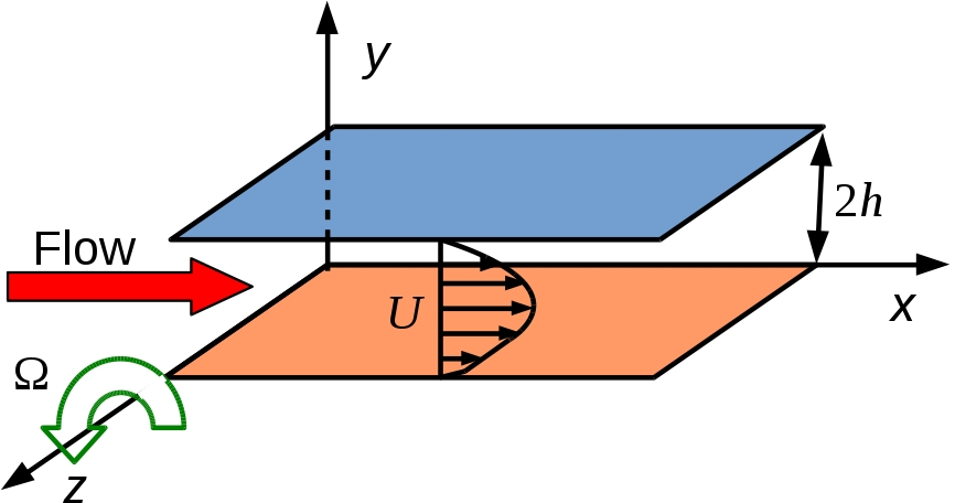
Figure 1: Flow configuration and coordinate system.

The incompressible Navier-Stokes equations (Brethouwer 2016) are solved with a pseudo-spectral code, as in Brethouwer (2016, 2017), with Fourier expansions in the streamwise $x$- and spanwise $z$-direction and Chebyshev polynomials in the wall-normal $y$-direction (Chevalier et al. 2007). Together with the Navier-Stokes, the code solves the advection-diffusion equation for a passive scalar

$$\frac{\partial\Theta^{\prime}}{\partial t}+\mathbf{U}^{\prime}\mathbf{\cdot}\mathbf{\nabla}\Theta^{\prime}=\frac{1}{Re\,Pr}\nabla^{2}\Theta^{\prime}$$ (1)

where $\mathbf{U}^{\prime}$ is the dimensionless velocity and $\Theta^{\prime}$ the scalar value. In the $x$- and $z$-direction, periodic boundary conditions are used for the the scalar and velocity, and no-slip conditions for the velocity at the walls. Further, $\Theta^{\prime}=0$ at one wall at $y=-1$ and $\Theta^{\prime}=1$ at the other wall at $y=1$, where $y$ is made non-dimensional with $h$. The scalar is thus kept at constant but different values at the wall, like in Johansson & Wikström (1999) and Nagano & Hattori (2003). In the statistically stationary state the mean scalar fluxes are equal at both walls.

In the DNS the flow rate and thus $Re$ was kept constant at $20\,000$ and $Pr=0.71$. The domain size was $8\pi h$, $2h$ and $3\pi$ in the $x$-, $y$- and $z$-direction, respectively, and the spatial resolution was similar as in other DNS of turbulent channel flow (Lee & Moser 2015). The rotation number $Ro$ was varied from 0 (no rotation) to a quite high value of 1.2. The parameters of the DNS are listed in table 1.

Table 1: DNS parameters: $N_{x}$, $N_{y}$ and $N_{z}$ are the number of modes in the streamwise, wall-normal and spanwise direction, respectively.

$Ro$	$Re_{\tau}$	$Re^{u}_{\tau}$	$Re^{s}_{\tau}$	$N_{x}\times N_{y}\times N_{z}$
0	1000	1000	1000	$2560\times 385\times 1920$
0.15	976	1107	825	$2304\times 385\times 1728$
0.45	800	964	594	$2048\times 361\times 1536$
0.65	700	851	505	$1920\times 321\times 1440$
0.9	544	677	365	$1536\times 257\times 1152$
1.2	423	501	326	$1152\times 217\times 864$

The friction velocity is defined as $u_{\tau}=[u^{2}_{\tau u}/2+u^{2}_{\tau s}/2]^{1/2}$, where $u_{\tau u}$ and $u_{\tau s}$ are the friction velocity of unstable and stable channel side, respectively (Grundestam et al. 2008). $Re^{u}_{\tau}$ and $Re^{s}_{\tau}$ are Reynolds numbers based on $u_{\tau u}$ and $u_{\tau s}$, respectively.

Before the statistics were collected, I ran the DNS for a sufficiently long time to reach a statistically stationary state with a constant mean scalar flux. I experienced that it can take a long time before the scalar field reaches such a state when the channel is rotating.

III 3. Flow field

Before I present and discuss the DNS results on the scalar transport I will briefly discuss some one-point flow statistics. A more comprehensive study of rotating channel flow is presented in Brethouwer (2016, 2017) and other publications cited in the Introduction. Note that in this paper I only show results for $Re=20\,000$ whereas in Brethouwer (2017) I often show results for other $Re$. Here below, $U$ denotes the mean streamwise velocity and $u$, $v$ and $w$ the streamwise, wall-normal and spanwise velocity fluctuations, respectively. An overbar implies averaging over time and homogeneous $x$- and $z$-directions.

Figure 2.(a) shows that all profiles of $U/U_{b}$ for $Ro>0$ are skewed and have a linear slope part with $\mbox{d}U/\mbox{d}y\simeq 2\Omega$ on the unstable side. In the DNS $y=-1$ and 1 correspond to the wall on the unstable and stable channel sides, respectively.

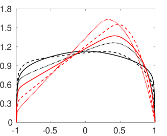
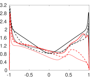
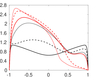
(a) (b) (c) (d)

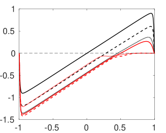
Figure 2: Profiles of (a) $U/U_{b}$, (b) $u^{+}$, (c) $v^{+}$, and (d) $uv^{+}$. ($~{}^{\line(1,0){20.0}}$) $Ro=0$, ($---$) $Ro=0.15$, ($\cdot\cdot\cdot$) $Ro=0.45$, (${\color[rgb]{1,0,0}~{}^{\line(1,0){20.0}}}$) $Ro=0.65$, (${\color[rgb]{1,0,0}---}$) $Ro=0.9$. (${\color[rgb]{1,0,0}\cdot\cdot\cdot}$) $Ro=1.2$.

Figure 2.(b) and (c) show the profiles of the root-mean-square of the streamwise and wall-normal velocity fluctuations $u^{+}$ respective $v^{+}$ scaled by $u_{\tau}$. On the stable side $u^{+}$ is strongly reduced by rotation and the sharp peak near the wall disappears. The maximum of $v^{+}$ grows, respectively, decays monotonically with $Ro$ on the unstable and stable channel side while the normalized Reynolds shear stress, $uv^{+}=\overline{uv}/u^{2}_{\tau}$, decays with $Ro$ on the stable side (figure 2.d). Both $v^{+}$ and $uv^{+}$ are small or nearly zero on the stable channel side if $Ro\geq 0.9$. When $Ro$ is further raised turbulence becomes also weak on the unstable side and if $Ro\geq 2.4$ turbulent momentum transfer is negligible and the flow approaches a laminar state (Brethouwer 2017). In the DNS $Re$ is constant but $Re_{\tau}$ varies and decreases with $Ro$, see table 1, owing to the reduced Reynolds stresses.

IV 4. Visualizations of the scalar field and time series

One-dimensional velocity spectra at $Re=20\,000$ and $Ro=0$, 0.15, 0.45 and 0.9 and visualizations of the instantaneous flow field are presented in Brethouwer (2017). These spectra and visualizations reveal the presence of large and long streamwise counter-rotating roll cells on the unstable channel side at $Ro=0.15$ with a spanwise size of $\pi h/2$. The roll cells leave an imprint on the scalar field visualized in figure 3. Whereas no clear coherent structures can be seen in the scalar field in the non-rotating channel (figure 3.a), at $Ro=0.15$ narrow streaks with low scalar values are observed in the $x$-$z$ plane on the unstable channel side in the outer layer (figure 3.b).

(a) (b) (c) (d) (e)

Figure 3: Visualizations of the instantaneous scalar field in an $x$-$z$ plane at (a) $Ro=0$ and $y=-0.6$, (b) $Ro=0.15$ and $y=-0.6$, (c) $Ro=0.45$ and $y=-0.8$, (d) $Ro=0.65$ and $y=-0.8$ and (e) $Ro=0.9$ and $y=-0.85$. Dark colours correspond to low scalar values.

These are approximately aligned with the flow direction and caused by updrafts between the counter rotating roll cells coming from the lower wall at $y=-1$. With increasing $Ro$ roll cells tend to become smaller and less obvious, accordingly, the streaks with low scalar values become less coherent and the spanwise distance between them diminishes (figure 3.c, d) and at $Ro=0.9$ roll cells are hardly perceptible (figure 3.e). These observations are consistent with the energy spectra presented in Brethouwer (2017).

Figure 4 shows the instantaneous scalar gradient on the wall at $y=1$ on the stable channel side.

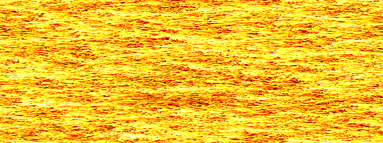
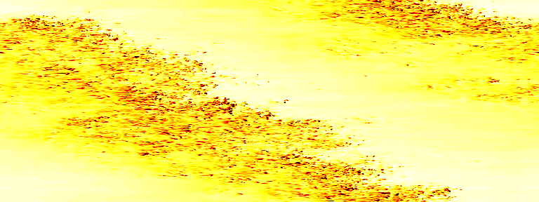
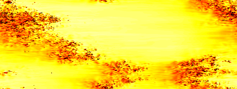
(a) (b) (c) (d) (e)

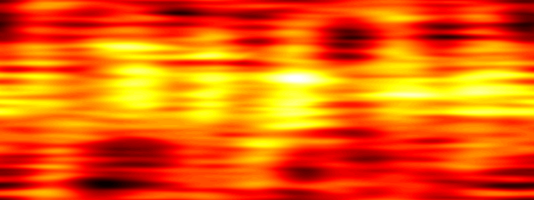
Figure 4: Visualizations of the instantaneous scalar gradient at $y=1$ at (a) $Ro=0$, (b) $Ro=0.15$, (c) $Ro=0.45$, (d) $Ro=0.65$ and (e) $Ro=0.9$. Dark colours correspond to high scalar gradients.

The fluctuations in the scalar gradient imply that the flow is fully turbulent here if $Ro\leq 0.15$ (figure 4.a, b), but at higher $Ro$ it starts to partly relaminarize on the stable channel side. At $Ro=0.45$ oblique banded patterns develop with alternating turbulent and laminar-like flow (Brethouwer 2017). A corresponding pattern emerges in the scalar gradient field with oblique banded regions with strong scalar gradient fluctuations induced by the turbulence and regions where these gradient fluctuations are mostly absent since the flow is locally laminar-like (figure 4.c). Similar oblique turbulent-laminar patterns have been observed in several flow types, see for example, Duguet et al. (2009), Brethouwer et al. (2012) and Deusebio et al. (2014). A distinguishing feature is that the patterns do not span the whole channel in the present case but are only found on the stable side. At a higher $Ro=0.65$ the patterns with turbulence and strong scalar gradient fluctuations become less coherent, as seen in figure 4.(d). They also appear to become more unsteady and their size varies in time, as indicated by other visualizations (not shown) and temporal variations in the mean scalar gradient and skin friction at $y=1$, shown later. When $Ro\geq 0.9$ fluctuations are weak on the stable side and small-scale fluctuations in the scalar gradient field cannot be observed (figure 4.e), implying that near-wall turbulence is suppressed by the system rotation.

Instantaneous plots of the scalar field in a $y$-$z$-plane at $Ro=0$, 0.45 and 0.9 are shown in figure 5.

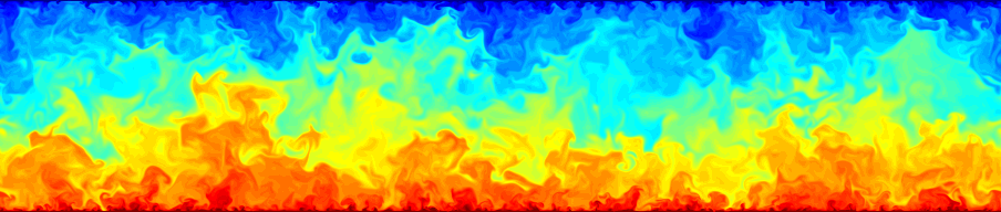
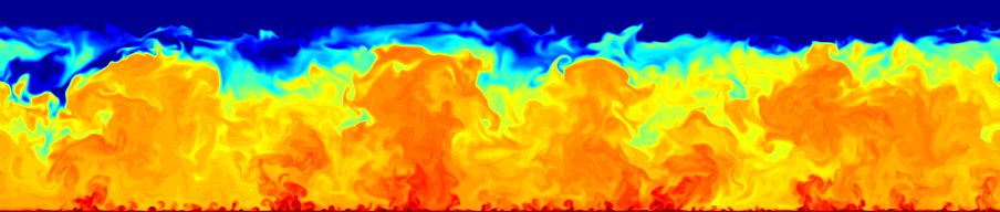
(a) (b) (c)

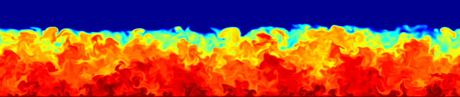
Figure 5: Visualizations of the instantaneous scalar field in a $y$-$z$-plane at (a) $Ro=0$, (b) $Ro=0.45$ and (c) $Ro=0.9$. Red and blue colours correspond to low and high scalar values, respectively.

At $Ro=0.45$, the visualization reveals large-scale plume-like structures in the scalar field (figure 5.b), which are likely caused by the large streamwise roll cells. At higher $Ro$ and $Ro=0$, the roll cells are absent or much smaller (Brethouwer 2017) and accordingly no or less large plumes are seen in the scalar field (figure 5.a, c). Large jumps in the scalar field are observed when $Ro>0$ in the core region near the border of stable and unstable channel side where the mean scalar gradient is large, as discussed later.

It is important to remark that at $Re=20\,000$ a linear instability of Tollmien-Schlichting-like waves occurs when $Ro\geq 0.9$ (Brethouwer 2016). This instability causes recurring bursts of turbulence mostly confined to the stable channel side and its mechanism is examined in Brethouwer et al. (2014) and Brethouwer (2016). The instability and strong bursts naturally affect the scalar field, as shown by the time series in figure 6.

(a)

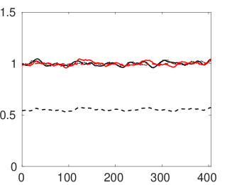
(c)

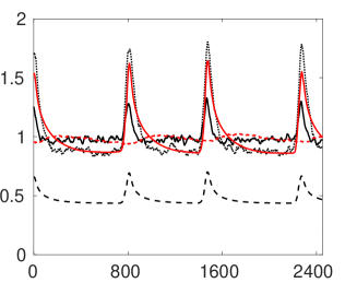
Figure 6: Time series at (a) $R=0.45$, (b) $R=0.65$, (c) $R=0.9$ and (d) $R=1.2$ of the volume averaged $K_{m}$ ($~{}^{\line(1,0){20.0}}$) and $\theta_{m}$ ($\cdot\cdot\cdot$), and wall gradients $\tau_{ws}$ ($---$), $(\mbox{d}\Theta/\mbox{d}y)_{u}$ (${\color[rgb]{1,0,0}---}$) and $(\mbox{d}\Theta/\mbox{d}y)_{s}$ (${\color[rgb]{1,0,0}~{}^{\line(1,0){20.0}}}$). $\tau_{ws}$ is normalized with the time-averaged wall shear on both wall whereas the other quantities are normalized with their respective time-averaged values.

In this figure, time series of the volume averaged turbulent kinetic energy $K_{m}$ and root-mean-square of the scalar fluctuations $\theta_{m}$ are presented as well as the wall shear stress $\tau_{ws}$ at $y=1$ and wall temperature gradients $(\mbox{d}\Theta/\mbox{d}y)_{u}$ and $(\mbox{d}\Theta/\mbox{d}y)_{s}$ at $y=-1$ and $y=1$, respectively. The stress and gradients are averaged over the wall and the time $t$ is scaled by $h/U_{b}$. When $Ro\leq 0.45$ all these quantities are approximately constant in time (figures 6.a) but at $Ro=0.65$, $\tau_{ws}$ and $(\mbox{d}\Theta/\mbox{d}y)_{s}$ display noticeable variations caused by the growing and shrinking of the turbulent areas on the stable channel side, as discussed before. Dai et al. (2016) have observed similar variations of $\tau_{ws}$ in their DNS and attributed these to the dynamics and changes of the streamwise roll cells. At $Ro=0.9$ and 1.2 the time series of $\theta_{m}$ and $(\mbox{d}\Theta/\mbox{d}y)_{s}$ show simultaneously with $K_{m}$ and $\tau_{ws}$ recurring sharp peaks with a time interval of about $700t$, whereas $(\mbox{d}\Theta/\mbox{d}y)_{u}$ and the wall shear stress at $y=-1$ (not shown) stay approximately constant. This shows that the bursts of turbulence triggered by the linear instability causes sharp and significant but relatively short surges in the scalar fluctuations and scalar flux at the wall on the stable channel side. Such recurring bursts are also observed at higher $Ro$. However, when $Ro\geq 2.1$ and the turbulence is weak in the whole channel (Brethouwer 2017) the bursts trigger sharp spikes in the scalar flux not only at the wall at $y=1$ but also at the other wall (not shown).

Although interesting, I will not further explore these recurring bursts in the DNS at $Ro\geq 0.9$ but focus in the rest of the paper in these DNS on the relatively calm periods between the bursts. From a modelling point of view these calm periods are more relevant and give a better fundamental insight into the influence of rotation on turbulent scalar transport. Including the bursts would add further complexity to the problem. I therefore compute the scalar statistics from the statistics collected during the calm periods between the bursts. In Brethouwer (2017) I explain in more detail how I exclude the periods with the bursts from the statistics.

V 5. Passive scalar transport

In this section, I will discuss the basic statistics of the scalar field and scalar transport. Here below, $\Theta$ is used to denote the mean scalar value, i.e. averaged over time and $x$- and $z$-directions, and $\theta$ the scalar fluctuation. A superscript $+$ implies, unless stated otherwise, scaling in terms of viscous wall units $\nu$ and $u_{\tau}$ and $\theta_{\tau}=Q_{w}/u_{\tau}$ where $Q_{w}=\alpha(\mbox{d}\Theta/\mbox{d}y)_{w}$ is the mean scalar flux at the wall, which is equal at both walls in the statistically stationary state.

Figure 7.(a) shows profiles of $\Theta$ at different $Ro$.

(a)

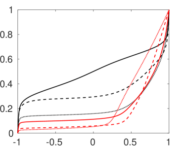
Figure 7: Profiles of (a) $\Theta$ and (b) $\theta^{+}$. Lines as in figure 2.

The mean scalar value $\Theta$ goes down monotonically with $Ro$ on the unstable channel side, whereas on the stable side the mean scalar gradient is steep in rotating channel flow, much steeper than on the unstable side. This can be understood by considering the mean scalar transport across the channel in the steady state

$$\alpha\frac{\mbox{d}\Theta}{\mbox{d}y}-\overline{v\theta}=Q_{w}.$$ (2)

On the stable channel side, $\overline{v\theta}$ is strongly diminished in rotating channel flow, as shown later, which naturally implies a large $\alpha\mbox{d}\Theta/\mbox{d}y$ to maintain the scalar flux balance. Profiles of the root-mean-square of the scalar fluctuations $\theta^{+}$ are shown in figure 7.(b). At $Ro=0$ the profile of $\theta^{+}$ has not only peaks near both walls caused by intense near-wall turbulence but also a maximum at the centre as a result of a large $\mbox{d}\Theta/\mbox{d}y$ and, consequently, a high production of scalar fluctuations here, as shown later. When $0.15\leq Ro\leq 0.65$, $\theta^{+}$ including the near-wall peak on the unstable channel side declines with $Ro$ and grows on the stable channel side. This growth is caused by the large $\mbox{d}\Theta/\mbox{d}y$ and related large production of scalar fluctuations on the stable side. Note that scalar fluctuations are strong although turbulence is weakened by rotation on the stable channel side. At higher $Ro$, $\theta^{+}$ declines in the near-wall region of the stable side. Instead, $\theta^{+}$ has a pronounced maximum near the position where $\mbox{d}\Theta/\mbox{d}y$ strongly increases going from the unstable towards the stable channel side. Quite similar trends regarding the profiles of $\Theta$ and $\theta^{+}$ are also observed at lower Reynolds numbers (Nagano & Hattori 2003, Liu & Lu 2007).

Figure 8 shows the mean velocity $U^{+}$ and scalar $\Theta^{+}$ profiles on the unstable channel side as function of the distance to the wall in wall units $y^{+}$.

(a)

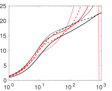
Figure 8: Profiles of (a) $U^{+}$ and (b) $\Theta^{+}$ as function of $y^{+}$. The straight green and blue dashed lines in (b) are explained in the text. Other lines as in figure 2.

The mean velocity profile at $Ro=0$ follows approximately a log-law behaviour between the near-wall and centre region, but a similar log-law behaviour is not observed when $Ro>0$ and cannot be expected from theoretical arguments since the velocity profile depends on $Ro$. Previous studies have shown that in the overlap region of non-rotating channel flow the $\Theta^{+}$-profile has a similar log-law behaviour as the velocity (Kawamura et al. 1999, Pirozzoli et al. 2016). Accordingly, in the present DNS at $Ro=0$, the mean scalar profile between the near-wall and centre region approximately matches

$$\Theta^{+}=\frac{1}{\kappa_{\theta}}\log\,y^{+}+C_{\theta}$$ (3)

with $\kappa_{\theta}=0.42$ and $C_{\theta}=2.8$ given by the straight green dashed line (figure 8.b). The present value of $\kappa_{\theta}=0.42$ is similar to the values 0.43 and 0.46 found by Kawamura et al. (1999), respectively, Pirozzoli et al. (2016). When $Ro\geq 0.45$ the profiles of $\Theta^{+}$ on the unstable side away from the wall approximately also follow the logarithmic profile (3) but with $\kappa_{\theta}=2.0$ and decreasing values of $C_{\theta}$ with $Ro$, given by the straight blue dashed lines in figure 8.(b), despite the absence of a similar log-law behaviour in the $U^{+}$-profile. A closer inspection shows that this log-law region partly overlaps with the region where the mean velocity profile is approximately linear and $\mbox{d}U/\mbox{d}y\approx 2\Omega$. Whether this log-law behaviour of the $\Theta^{+}$-profiles with the same logarithmic slope in rotating channel flows is just a coincidence is not yet clear and there is obvious explanation for this behaviour.

I will now consider turbulent scalar transport. Figure 9.(a) and (b) show the profiles of the streamwise and wall-normal turbulent scalar fluxes $\overline{u\theta}^{+}$ respective $\overline{v\theta}^{+}$ in wall units.

(a)

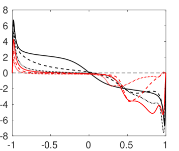
(c)

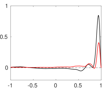
Figure 9: Profiles of (a) $\overline{u\theta}^{+}$ and (b) $\overline{v\theta}^{+}$. Lines as in figure 2. (c) Profile of $\overline{w\theta}^{+}$ at (${~{}^{\line(1,0){20.0}}}$) $Ro=0.45$ $Ro=0.45$ and (${\color[rgb]{1,0,0}~{}^{\line(1,0){20.0}}}$) $Ro=0.65$.

In non-rotating channel flow $\overline{u\theta}^{+}$ has, except around the centreline, a larger magnitude than $\overline{v\theta}^{+}$ (Johansson & Wikström 1999) meaning that the turbulent scalar flux is mainly aligned with the streamwise direction and the same applies to the stable channel side in the rotating cases. When $Ro$ rises, $\overline{u\theta}^{+}$ including its near-wall peak monotonically declines on the unstable side while $-\overline{v\theta}^{+}$ stays near unity, meaning that the turbulent scalar flux vector turns towards the wall-normal direction and is nearly aligned with the wall-normal direction away from the wall in the region where $\mbox{d}U/\mbox{d}y\approx 2\Omega$. On the stable channel side, $-\overline{v\theta}^{+}$ declines with $Ro$ and is very small for $Ro\geq 0.9$ when the flow relaminarizes there, whereas $\overline{u\theta}^{+}$ stays large for $Ro\leq 0.65$ but declines at higher $Ro$ and its near-wall peak disappears (figure 9). The scalar transport on the stable channel side is thus mainly diffusive at higher $Ro$. These results are consistent with previous DNS of scalar transport in rotating channel flow at lower $Re$ and with a smaller range of $Ro$ (Nagano & Hattori 2003, Liu & Lu 2007). They are also consistent with DNS and rapid distortion theory of homogeneous turbulent shear flow subject to spanwise system rotation. In that case, the turbulent scalar flux vector is mostly aligned with the streamwise direction when the rotation is absent, or cyclonic as on the stable channel side. When the rotation is anti-cyclonic as on the unstable channel side the turbulent scalar flux vector becomes more aligned with the wall-normal direction and is almost fully aligned with the mean scalar gradient when the mean shear $\mbox{d}U/\mbox{d}y$ equals $2\Omega$, where $\Omega$ is the imposed rotation (Brethouwer 2005, Kassinos et al. 2007), like in the present case.

In non-rotating turbulent channel flow the mean spanwise turbulent scalar flux $\overline{w\theta}^{+}$ is naturally zero. But figure 9.(c) shows that when $Ro=0.45$ or 0.65 and oblique turbulent patterns are present in the near-wall region of the stable side (figure 4.c, d) $\overline{w\theta}^{+}$ is significant in this region. In these cases, $\overline{uw}$ is also non-zero. The oblique patterns induce thus a noticeable spanwise turbulent momentum and scalar transport near the wall.

Figure 10 shows the correlation coefficients $\rho_{u\theta}=\overline{u\theta}/(u^{\prime}\theta^{\prime})$ and $\rho_{v\theta}=-\overline{v\theta}/(v^{\prime}\theta^{\prime})$, where a prime ^′ denotes root-mean-square values.

(a)

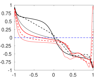
(c)

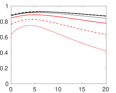
Figure 10: Profiles of (a,c) $\rho_{u\theta}$ and (b,d) $\rho_{v\theta}$, (c) and (d) show a close-up near the wall on the unstable side. Lines as in figure 2.

Consistent with Abe & Antonia (2009) and Pirozzoli et al. (2016), very high streamwise flux correlations $\rho_{u\theta}$ are found at $Ro=0$ near the wall owing the very high similarity between the streamwise velocity and scalar field (figure 10.c), while in the outer layer, except around the centreline, $\rho_{u\theta}$ is lower yet still large (figure 10.a). A large correlation means here large positive or large negative values of $\rho_{u\theta}$. In the rotating cases, the magnitude of $\rho_{u\theta}$ remains large on the stable channel side, but on the unstable side it declines rapidly in the outer layer with $Ro$ and even becomes negative at high $Ro$ (figure 10.a). Close to the wall on the unstable side, $\rho_{u\theta}$ declines when $Ro\geq 0.65$ but remains quite large (figure 10.c). Thus, rotation reduces the similarity between the $u$- and $\theta$-field on the unstable side, especially in the outer layer. Yang et al. (2011) came to a similar conclusion for DNS of rotating channel flow at much lower $Re$. The high near-wall correlation at $Ro=0$ is motivated by the similarity between the governing equations for $u$ and $\theta$ with the main difference being the pressure gradient term (Abe & Antonia 2009). However, if $Ro>0$ an additional Coriolis term appears in the former, which diminishes the similarity between the governing equations and, accordingly, the correlation between $u$ and $\theta$.

By contrast, $\rho_{v\theta}$ is quite insensitive to $Ro$ on the unstable channel side away from the wall with values between 0.4 and 0.5 whereas it declines with $Ro$ on the stable side (figure 10.b). On the other hand, near the wall on the unstable side, $\rho_{v\theta}$ increases considerably with $Ro$ and becomes quite large (figure 10.d). The behaviour and magnitude of $\rho_{v\theta}$ with $Ro$ follows here closely the correlation coefficient for the Reynolds shear stress $\overline{uv}/(u^{\prime}v^{\prime})$ (not shown) which also becomes large near the wall at higher $Ro$. These high correlations might be related to the formation of elongated streamwise near-wall vortices in rotating channel flow on the unstable side (Yang & Wu 2012).

To conclude, the alignment of the scalar flux with the mean scalar gradient with $Ro$ on the unstable side is related to the reduced correlation between streamwise velocity and scalar fluctuations whereas the reduced turbulent scalar fluxes on the stable side are caused by both declining $v$-$\theta$ correlations and Reynolds stresses.

Figure 11 shows the near-wall peak values of $u^{+}$ and $\theta^{+}$ as function of $Ro$.

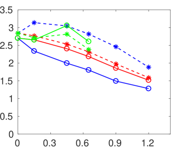
Figure 11: The maximum near-wall value of $u^{+}$ ($\ast---\ast$) and $\theta^{+}$ ($\circ^{\line(1,0){1.0}}\circ$) on the unstable (blue and red lines/symbols) and stable channel side (green lines/symbols) as function of $Ro$. Blue lines and symbols: using wall units based on $u_{\tau}$. Red lines and symbols: using wall units based on $u_{\tau u}$. Green lines and symbols: using wall units based on $u_{\tau s}$.

The velocity and scalar fluctuations on the unstable side are either scaled by $u_{\tau}$ and $\theta_{\tau}=Q_{w}/u_{\tau}$, respectively, or by $u_{\tau u}$ and $\theta_{\tau u}=Q_{w}/u_{\tau u}$, respectively, while on the stable channel side they are scaled by $u_{\tau s}$ and $\theta_{\tau s}=Q_{w}/u_{\tau s}$, respectively. The high similarity between the $u$ and $\theta$ field in the near-wall region in non-rotating channel flow (Abe & Antonia 2009) is reflected by the closeness of the peak values of $u^{+}$ and $\theta^{+}$, although the peak value of $u^{+}$ is slightly higher than that of $\theta^{+}$, as a consequence of a smaller than unity $Pr$ (Pirozzoli et al. 2016). In rotating channel flow the difference between the peak values of $u^{+}$ and $\theta^{+}$ is considerable if the scaling is based on $u_{\tau}$ and $\theta_{\tau}$, but if the scaling of the peak values on the unstable and stable channel side is based on $u_{\tau u}$, $\theta_{\tau u}$ and $u_{\tau s}$, $\theta_{\tau s}$, respectively, the differences are much smaller. In the latter case, the peak values of $u^{+}$ and $\theta^{+}$ on the unstable channel side show a very similar downward trend with $Ro$. The trend on the stable channel side is non-monotonic, which may be related to the appearance of turbulent-laminar patterns at $Ro=0.45$ and 0.65. Rotation reduces thus the similarity between the $u$- and $\theta$-field on the unstable side, but their near-wall peak values are still highly correlated and display a similar scaling in terms of wall units.

VI 6. Budget equations

In this section, the budgets of the governing equations of the scalar energy $K_{\theta}=\frac{1}{2}\overline{\theta\theta}$ and $\overline{u\theta}$ and $\overline{v\theta}$ are considered to obtain insights into the generation of scalar fluctuations and fluxes. Budgets for scalar transport in non-rotating channel have been studied by e.g. Johansson & Wikström (1999) and in spanwise rotating channel flow by Nagano & Hattori (2003) and Liu & Lu (2007), albeit at low Reynolds numbers.

In the present steady-state case, the governing equation of the scalar energy $K_{\theta}$ reads

$$0=\underbrace{-\overline{v\theta}\frac{\partial\Theta}{\partial y}}_{P_{\theta}}\underbrace{-\frac{1}{2}\frac{\partial\overline{v\theta^{2}}}{\partial y}}_{D^{t}_{\theta}}+\underbrace{\alpha\frac{\partial^{2}K_{\theta}}{\partial y^{2}}}_{D^{m}_{\theta}}\underbrace{-\alpha\overline{\frac{\partial\theta}{\partial x_{k}}\frac{\partial\theta}{\partial x_{k}}}}_{\varepsilon_{\theta}},$$ (4)

where $P_{\theta}$ represents production, $D^{t}_{\theta}$ and $D^{m}_{\theta}$ turbulent and molecular diffusion, respectively, and $\varepsilon_{\theta}$ dissipation. Figure 12 shows the budgets $P^{+}_{\theta}$, $D^{t+}_{\theta}$ and $\varepsilon^{+}_{\theta}$ in wall units at $Ro=0$, 0.15, 0.65 and 1.2. The molecular diffusion $D^{m}_{\theta}$ is not shown since it is small.

(a)

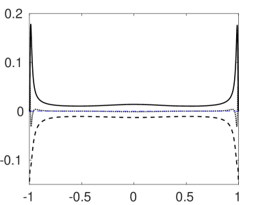
(c)

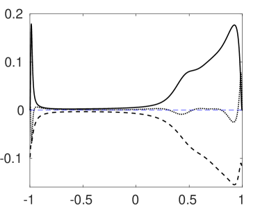
Figure 12: Budgets of the $K_{\theta}$-balance equation in wall units at (a) $Ro=0$, (b) $Ro=0.15$, (c) $Ro=0.65$ and (d) $Ro=1.2$. ($~{}^{\line(1,0){20.0}}$) $P^{+}_{\theta}$, ($---$) $\varepsilon^{+}_{\theta}$, ($\cdot\cdot\cdot$) $D^{t+}_{\theta}$.

The turbulent diffusion $D^{t}_{\theta}$ appears only significant near the wall and at $Ro=1.2$ in the region away from the wall where $K_{\theta}$ and $P_{\theta}$ are large, implying that there is primarily a balance between $P_{\theta}$ and $\varepsilon_{\theta}$. Accordingly, at $Ro=0$ and $Ro\geq 0.9$ the ratio $P_{\theta}/\varepsilon_{\theta}$ is near unity in the outer region away from the border between the stable and unstable channel side (figure 13.b).

(a)

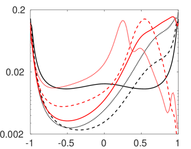
Figure 13: Profiles of (a) $\varepsilon^{+}_{\theta}$ and (b) $P_{\theta}/\varepsilon_{\theta}$. Lines as in figure 2.

However, $P^{+}_{\theta}$ and $\varepsilon^{+}_{\theta}$ are both very small on the unstable side away from the wall when $0.15\lesssim Ro\lesssim 0.65$ (figure 13.a) since the mean scalar gradient is small. In these cases the ratio $P_{\theta}/\varepsilon_{\theta}$ deviates significantly from unity (figure 13.b) implying that $D^{t}_{\theta}$ is significant. This disbalance between $P_{\theta}$ and $\varepsilon_{\theta}$ and the considerable diffusion of $K_{\theta}$ are likely caused by the large-scale streamwise roll cells being present at these rotation rates but which are much less dominant at higher $Ro$ (Brethouwer 2017). Liu & Lu (2007) show that these roll cells indeed have a large impact on scalar transport in rotating channel flows. The maximum value of $P^{+}_{\theta}$ close to the walls is independent of $Ro$ and close to its theoretical value $Pr/4$ (Johansson & Wikström 1999). At $Ro=0.15$ and even more so at $Ro=0.65$, both $\varepsilon^{+}_{\theta}$ and $P^{+}_{\theta}$ are large on the stable channel side (figure 12.b, c) where also the mean scalar gradient and $K_{\theta}$ are large (figure 7). At higher $Ro$, the peaks of $\varepsilon^{+}_{\theta}$ and $P^{+}_{\theta}$ on the stable side move away from the wall to the position, going from the unstable towards the stable side, where $\mbox{d}\Theta/\mbox{d}y$ steepens while $\overline{v\theta}$ is still large (figure 12.d). Accordingly, the maximum of $\theta^{+}$ at high $Ro$ moves away from the wall at high $Ro$ (figure 7.b). Moving closer to the wall on the stable side, $\overline{v\theta}$ and consequently $P^{+}_{\theta}$ and $\varepsilon^{+}_{\theta}$ diminish rapidly.

The respective governing equations of $\overline{u\theta}$ and $\overline{v\theta}$ read in the present case

$$0 = \underbrace{-\overline{uv}\frac{\partial\Theta}{\partial y}-\overline{v\theta}\frac{\partial U}{\partial y}}_{P_{1}}\underbrace{-\frac{\partial\overline{uv\theta}}{\partial y}}_{D^{t}_{1}}+\underbrace{\frac{\partial}{\partial y}\left(\alpha\overline{u\frac{\partial\theta}{\partial y}}+\nu\overline{\theta\frac{\partial u}{\partial y}}\right)}_{D^{m}_{1}}+\underbrace{\overline{\frac{p}{\rho}\frac{\partial\theta}{\partial x}}-(\alpha+\nu)\overline{\frac{\partial u}{\partial x_{k}}\frac{\partial\theta}{\partial x_{k}}}}_{\Pi_{1}}+\underbrace{2\Omega\overline{v\theta}}_{C_{1}}$$ (5)

$$0 = \underbrace{-\overline{v^{2}}\frac{\partial\Theta}{\partial y}}_{P_{2}}\underbrace{-\frac{\partial\overline{v^{2}\theta}}{\partial y}}_{D^{t}_{2}}\underbrace{-\frac{\partial\overline{p\theta}}{\partial y}}_{D^{p}_{2}}+\underbrace{\frac{\partial}{\partial y}\left(\alpha\overline{v\frac{\partial\theta}{\partial y}}+\nu\overline{\theta\frac{\partial v}{\partial y}}\right)}_{D^{m}_{2}}+\underbrace{\overline{\frac{p}{\rho}\frac{\partial\theta}{\partial y}}-(\alpha+\nu)\overline{\frac{\partial v}{\partial x_{k}}\frac{\partial\theta}{\partial x_{k}}}}_{\Pi_{2}}\underbrace{-2\Omega\overline{u\theta}}_{C_{2}}$$ (6)

where $P_{1}$, $P_{2}$ represent production, $D^{t}_{1}$, $D^{t}_{2}$ turbulent diffusion, $D^{p}_{2}$ pressure diffusion, and $D^{m}_{1}$, $D^{m}_{2}$ molecular diffusion. The sum of pressure scalar-gradient correlation and diffusive and viscous dissipation, $\Pi_{1}$ and $\Pi_{2}$, is considered because diffusive and viscous dissipation are generally considered to be small and therefore often added to the pressure scalar-gradient correlation term in turbulence modelling (Wikström et al. 2000). The Coriolis force leads to the additional terms $C_{1}$ and $C_{2}$ in the governing equations of the scalar fluxes.

Figure 14 shows the budgets $P^{+}_{1}$, $\Pi^{+}_{1}$, $D^{t+}_{1}$ and $C^{+}_{1}$ of the governing equation (5) of $\overline{u\theta}$ in wall units at $Ro=0$, 0.15, 0.65 and 1.2. The molecular diffusion $D^{m}_{1}$ is again not shown because of its smallness.

(a)

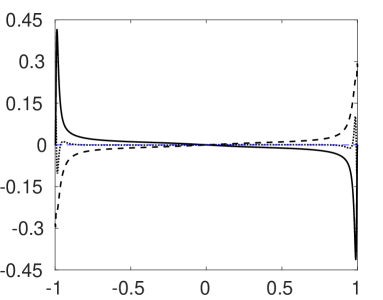
(c)

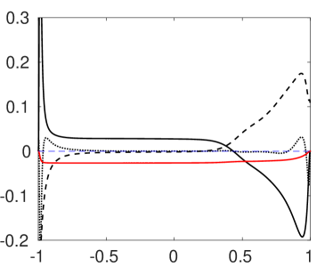
Figure 14: Budgets of the $\overline{u\theta}$-balance equation in wall units at (a) $Ro=0$, (b) $Ro=0.15$, (c) $Ro=0.65$ and (d) $Ro=1.2$. ($~{}^{\line(1,0){20.0}}$) $P^{+}_{1}$, ($---$) $\Pi^{+}_{1}$, ($\cdot\cdot\cdot$) $D^{t+}_{1}$, (${\color[rgb]{1,0,0}~{}^{\line(1,0){20.0}}}$) $C^{+}_{1}$.

At $Ro=0$, $P^{+}_{1}$ is in the whole channel mainly balanced by $\Pi^{+}_{1}$ and the same applies to the near wall region at $Ro=0.15$ (figure 14.a, b). When $-0.6\lesssim y\lesssim 0.4$ all budget terms are small in the latter case, but a closer inspection reveals that the Coriolis term $C^{+}_{1}$ is of the same order as $P^{+}_{1}$ and $\Pi^{+}_{1}$ and negative since $\overline{v\theta}$ is negative. At a higher $Ro=0.65$, $P^{+}_{1}$ and $\Pi^{+}_{1}$ are large and approximately balance each other in the near-wall region on the unstable side and a large part of the stable side (figure 14.c). On the other hand, in the outer region of the unstable side, $C^{+}_{1}$ is significant and balanced by $P^{+}_{1}$ and contributes to a small $\overline{u\theta}$ in this part of the channel (figure 9.a). When $Ro$ is raised to 1.2 turbulence disappears on the stable side and all budget terms are small there (figure 14.d). In the major part of the unstable channel side $D^{t+}_{\theta}$ and $\Pi^{+}_{1}$ are small but $P^{+}_{1}$ and $C^{+}_{1}$ are both large and balance each other. The balance of $P^{+}_{1}$ and $C^{+}_{1}$ in rotating channel flow on the unstable channel side can be understood by considering the production term more closely. This term has two contributions, namely $-\overline{uv}(\partial\Theta/\partial y)$ and $-\overline{v\theta}(\partial U/\partial y)$, see equation (5). The first part is small on the unstable side away from the wall because $\partial\Theta/\partial y$ is small. The second part $-\overline{v\theta}(\partial U/\partial y)$ is large but is nearly balanced by $C_{1}=\overline{v\theta}2\Omega$ since $\partial U/\partial y\approx 2\Omega$ on the unstable side. The term induced by the Coriolis force has thus a major impact on the streamwise scalar flux and contributes to the alignment between the turbulent scalar flux vector and mean scalar gradient in rotating channel flow.

Figure 15 shows the budgets $P^{+}_{2}$, $\Pi^{+}_{2}$, the sum $D^{t+}_{2}+D^{p+}_{2}$ and $C^{+}_{2}$ in the governing equation (6) of $\overline{v\theta}$ in wall units at $Ro=0$, 0.15, 0.65 and 1.2. The molecular diffusion $D^{m}_{2}$ is again small.

(a)

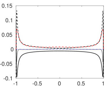
(c)

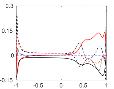
Figure 15: Budgets of the $\overline{v\theta}$-balance equation in wall units at (a) $Ro=0$, (b) $Ro=0.15$, (c) $Ro=0.65$ and (d) $Ro=1.2$. ($~{}^{\line(1,0){20.0}}$) $P^{+}_{2}$, ($---$) $\Pi^{+}_{2}$, ($\cdot\cdot\cdot$) $D^{t+}_{2}+D^{p+}_{2}$, (${\color[rgb]{1,0,0}---}$) $\Pi^{+}_{2}+D^{p+}_{2}$, (${\color[rgb]{1,0,0}~{}^{\line(1,0){20.0}}}$) $C^{+}_{2}$.

At $Ro=0$ the dominant contributions come from $P^{+}_{2}$ and $\Pi^{+}_{2}$, except very near the walls and near the centreline where diffusion $D^{t+}_{2}+D^{p+}_{2}$ is significant. At $Ro=0.15$ diffusion and $C^{+}_{2}$ are significant as well as $P^{+}_{2}$ and $\Pi^{+}_{2}$ in the main part of the channel. The Coriolis term $C^{+}_{2}$ contributes to the production of negative $\overline{v\theta}$ on the unstable side but counteracts it on the stable channel side since $\overline{u\theta}$ changes sign. At a higher $Ro=0.65$, $C^{+}_{2}$ is important and large on the stable side and near the wall on the unstable side but small away from the wall since $\overline{u\theta}$ is small. In a large part of the unstable channel side there is thus primarily a balance between $P^{+}_{2}$ and $\Pi^{+}_{2}$. At a higher $Ro=1.2$, $P^{+}_{2}$ is nearly constant away from the wall on the unstable side and balanced by $\Pi^{+}_{2}$ and $C^{+}_{2}$ while it rapidly declines approaching the wall on the stable channel side where both $\Pi^{+}_{2}$ and $C^{+}_{2}$ are large (figure 15.d). Note that $C_{2}$ is positive on the stable side in rotating channel flow and thus contributes to the reduced wall-normal turbulent scalar transport on that side. On the stable channel side, both $\Pi^{+}_{2}$ and diffusion dominated by $D^{p+}_{2}$ display large variations at $Ro=0.65$ and 1.2. By contrast, the profile of the sum $\Pi^{+}_{2}+D^{p+}_{2}=-((\overline{\theta\partial p}/\partial y)/\rho)^{+}$, which is also displayed in figure 15, is much smoother and does not show extreme values near the wall in rotating channel flow. This suggests that it might be easier to model the latter term instead of $\Pi_{2}$ and $D^{p}_{2}$ separately.

Figure 16 shows in more detail the production terms of turbulent kinetic energy $P_{K}$ and $P_{\theta}$ near the wall on the unstable side at $Ro=0$ and 0.65. Furthermore, the figure shows the sum $P_{2}+C_{2}$, which can be regarded as a total production of $\overline{v\theta}$, and $P_{1\theta}=-\overline{uv}(\partial\Theta/\partial y)$ and $P_{1u}=\overline{v\theta}(2\Omega\overline{v\theta}-\partial U/\partial y)$, which are the production owing to the mean scalar gradient, respective, the production by mean shear together with Coriolis term contribution in the governing equation (5) of $\overline{u\theta}$. The latter term, $P_{1u}$, is small away from the wall on the unstable side of a rotating channel when $\partial U/\partial y\approx 2\Omega$, as explained before. All terms and the distance to the wall $y^{*}$ are in wall units. The production terms are premultiplied by $y^{*}$ to accentuate the behaviour away from the wall. Here, $u_{u\tau}$ is used instead of $u_{\tau}$ for the scaling at $Ro=0.65$ because this velocity scale is more appropriate on the unstable side.

(a)

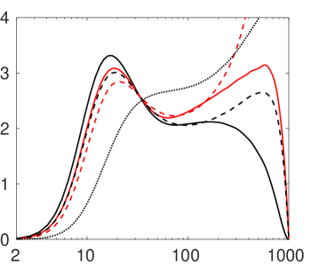
Figure 16: Premultiplied production terms in wall units on the unstable side at (a) $Ro=0$ and (b) $Ro=0.65$. ($~{}^{\line(1,0){20.0}}$) $y^{*}P^{*}_{K}$, (${\color[rgb]{1,0,0}---}$) $y^{*}P^{*}_{\theta}$, ($---$) $y^{*}P^{*}_{1\theta}$, (${\color[rgb]{1,0,0}~{}^{\line(1,0){20.0}}}$) $y^{*}P^{*}_{1u}$, ($\cdot\cdot\cdot$) $y^{*}(P^{*}_{2}+C^{*}_{2})$.

A DNS of scalar transport with $Pr=1$ in a non-rotating channel flow (not presented here) shows that the profiles of $P^{*}_{K}$, $P^{*}_{\theta}$, $P^{*}_{1\theta}$ and $P^{*}_{1u}$ including the maxima all collapse near the wall, see also Pirozzoli et al. (2016). Figure 16.(a) shows that in the present case with $Pr=0.71$ the profiles do not collapse when $Ro=0$ since the maximum of $P^{*}_{K}$ approaches $1/4$ whereas the maximum of $P^{*}_{\theta}$ is $Pr/4$ as explained before. The maxima of $P^{*}_{1\theta}$ and $P^{*}_{1u}$ are in between these two previous maxima and approximately equal to each other, showing that production owing to the mean scalar gradient and mean shear are equally important. All these maxima are nearly independent of $Ro$ (compare figure 16.a and b). The profiles of $P^{*}_{1\theta}$ and $P^{*}_{1u}$ approximately collapse for $y^{*}\lesssim 20$ (figure 16.b), also at other $Ro$, while they do not collapse if the Coriolis term is not included in $P^{*}_{1u}$, which is somewhat remarkable.

VII 7. Efficiency of scalar transport

In this section, some quantities characterising the efficiency of scalar transport are discussed; some of them are directly relevant for engineering.

An important quantity in engineering is the Nusselt number. It is here defined as the ratio of wall-normal scalar flux in the present turbulent channel flows and laminar channel flow, i.e.

$$Nu=\frac{2h}{\alpha\Delta\Theta}Q_{w},$$ (7)

where $\Delta\Theta$ is the imposed scalar difference at the walls. With this definition, $Nu=1$ for laminar channel flow.

However, $Nu$ does not distinguish between the scalar transport on the stable and unstable channel sides. To examine the effectivity of scalar transport on both channel sides, I have also computed a Nusselt number defined similarly as in some previous studies, e.g. Pirozzoli et al. (2016), to account for difference in the mean scalar gradients on both sides. For the unstable channel side it is defined as

$$Nu^{*}_{u}=\frac{5}{8}Q_{w}\frac{\delta}{\alpha|\Theta_{w}-\Theta_{m}|}.$$ (8)

Here, $\delta=y_{0}-y_{w}$ where $y_{0}$ is the position where the total shear stress, i.e. the sum of the viscous and turbulent shear stress, is zero, and $y_{w}$ the wall position and $\Theta_{w}$ the scalar value at the wall on the unstable channel side. I consider $y_{0}$ the place separating the stable and unstable channel sides. Further

$$\Theta_{m}=\frac{1}{\delta}\int^{y_{0}}_{y_{w}}\frac{U\Theta}{U_{m}}\mbox{d}y,~{}~{}~{}~{}~{}U_{m}=\frac{1}{\delta}\int^{y_{0}}_{y_{w}}U\mbox{d}y.$$ (9)

The Nusselt number for the stable channel side, $Nu^{*}_{s}$, is defined in the same way with the integrals in (9) from $y_{0}$ to $y_{w}$ where $y_{w}$ and $\Theta_{w}$ are now the wall position and the scalar value at the wall on the stable channel side. The factor $5/8$ in (8) and in the similar expression for $Nu^{*}_{s}$ ensures that $Nu^{*}_{u}=Nu^{*}_{s}=1$ if the flow is laminar. The main difference between the expressions for $Nu$ and $Nu^{*}_{u}$, $Nu^{*}_{s}$ is that $\Delta\Theta/2h$ is replaced by $|\Theta_{w}-\Theta_{m}|/\delta$ as an effective mean scalar gradient to characterize both channel sides.

(a)

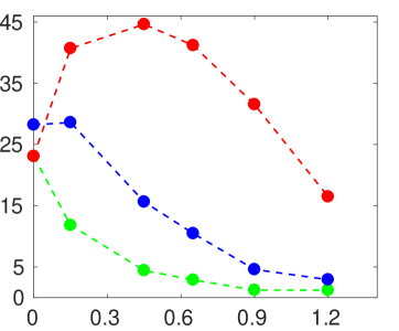
Figure 17: (a) $Nu$ (blue line/symbols), $Nu^{*}_{u}$ (red line/symbols) and $Nu^{*}_{s}$ (green line/symbols). (b) $2St/C_{f}$ on the unstable (red line/symbols) and stable channel side (green line/symbols).

Figure 17(a) shows $Nu$ together with $Nu^{*}_{u}$ and $Nu^{*}_{s}$ as function of $Ro$. $Nu$ slightly grows at first but then declines rapidly with $Ro$, implying that rotation drastically inhibits the cross channel scalar transport. The behaviour of $Nu$ in the present case is different from that in a rotating channel flow at a lower $Re_{\tau}=194$ when $Nu$ monotonically decreases with $Ro$ (Liu & Lu 2007). The high values of $Nu^{*}_{u}$ for $0.15\leq Ro\leq 0.9$ and rapid decline of $Nu^{*}_{s}$ with $Ro$ reflect the rapid and slow turbulent scalar transport on the unstable and stable channel sides, respectively. Both $Nu$ and $Nu^{*}_{s}$ approach unity at high $Ro$ meaning that diffusive scalar transport becomes significant.

Figure 17(b) shows the ratio of the Stanton number to skin friction coefficient $2St/C_{f}$ where

$$St=\frac{Q_{w}}{U_{m}T_{m}},~{}~{}~{}~{}~{}C_{f}=\frac{2u^{2}_{\tau}}{U_{m}}.$$ (10)

Here, $U_{m}$, $T_{m}$ and $u_{\tau}$ are either computed for the unstable or the stable channel side according to equation (9). If the Reynolds analogy for the momentum and scalar transport is valid $2St/C_{f}$ should be near unity (Abe & Antonia 2017), which indeed it is in the non-rotating channel (figure 17.b). On the stable channel side $2St/C_{f}$ stays near unity while on the unstable channel side it grows with $Ro$ and clearly deviates from unity, suggesting that the Reynolds analogy is valid for the stable channel side but not for the unstable side where scalar transport is relatively rapid.

The ratio of scalar to turbulence time-scale

$$r=\frac{K_{\theta}/\varepsilon_{\theta}}{K/\varepsilon}$$ (11)

is in some turbulence models assumed to be a constant. Antonia et al. (2009) found that in non-rotating turbulent channel flow with a passive scalar with $Pr=0.71$, $r$ is indeed nearly constant; its value is between 0.5 and 0.6 in the outer region. In rotating homogeneous shear flow, however, $r$ varies with the imposed system rotation rate (Brethouwer 2005). Figure 18(a) shows the profiles of $r$ in rotating channel flow.

(a)

(c)

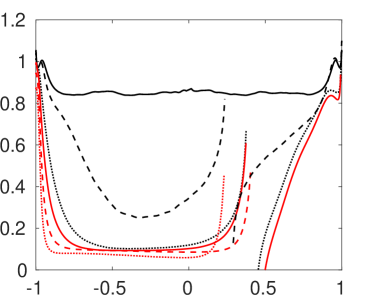
Figure 18: Profiles of (a) $r$, (b) $B$ and (c) $Pr_{T}$. Lines as in figure 2.

The variation of $r$ across the channel in the present DNS at $Ro=0$ is larger than in the DNS by Antonia et al. (2009), which is the consequence of a different forcing of the scalar field in those two DNS. Nevertheless, in the outer region but outside the centre region $r$ is close to that observed by Antonia et al. (2009). In rotating channel flow, $r$ at first grows with $Ro$ and varies between 0.7 and 0.85 at $Ro=0.15$, but then declines somewhat on the unstable channel side and varies there between approximately 0.6 and 0.7. Thus, the time-scale ratio $r$ displays some variations with $Ro$ but these are not very large.

A measure of turbulence to scalar fluctuation intensity is given by the dimensionless parameter

$$B=\frac{\sqrt{K}/\mbox{d}U/\mbox{d}y}{\sqrt{K}_{\theta}/\mbox{d}\Theta/\mbox{d}y}$$ (12)

Figure 18(b) shows the profiles of $B$ in the present DNS. The values of $B$ of approximately 1.2 to 1.3 at $Ro=0$ in the outer regions $-0.95\lesssim y\lesssim-0.6$ and $0.4\lesssim y\lesssim 0.95$ are the same as those observed by Antonia et al. (2009) in their DNS of non-rotating turbulent channel flow at similar $Re$. In the centre region, $B$ is much larger in the present DNS since the mean velocity gradient is small, unlike the fluctuations and mean scalar gradient. With increasing $Ro$, however, $B$ declines strongly in the outer region of the unstable channel side to less than 0.4, meaning that rotation augments scalar fluctuations relative to velocity fluctuations. The same trend is observed in rotating homogeneous shear flow with a passive scalar (Brethouwer 2005). Especially when the mean shear $\mbox{d}U/\mbox{d}y$ equals $2\Omega$, as in the absolute mean vorticity region in the present DNS, scalar fluctuations are relatively strong, although neither in the governing equation of $K$ nor $K_{\theta}$ there is a direct influence of rotation. The small values of $B$ in rotating channel flow, however, suggest that $P_{\theta}$ is relatively large compared to the production of $K$.

An important parameter in turbulence modelling, often assumed to be a constant, is the ratio of turbulent viscosity to scalar diffusivity given by the turbulent Prandtl number

$$Pr_{T}=\frac{\nu_{T}}{\alpha_{T}}=\frac{\overline{uv}}{\overline{v\theta}}\frac{\mbox{d}\Theta/\mbox{d}y}{\mbox{d}U/\mbox{d}y}.$$ (13)

It can also be considered as a relative measure of the production term of $K$ to $K_{\theta}$. Figure 18(c) shows the profiles of $Pr_{T}$ obtained from the present DNS. At $Ro=0$, $Pr_{T}\simeq 0.85$ in the outer region, consistent with the values computed by Antonia et al. (2009) and Pirozzoli et al. (2016) for non-rotating channel flow. On the other hand, in rotating channel flow $Pr_{T}$ is considerably smaller in the outer region of the unstable channel side; it is less than 0.2 for $Ro\geq 0.45$. Also on the stable channel side at $Ro=0.15$, $Pr_{T}$ is smaller than in the non-rotating case away from the wall. These results show, like the ratio $2St/C_{f}$ in figure 17.(b), that the Reynolds analogy for scalar-momentum transfer does not hold for rotating channel flow and that turbulent scalar transport is very efficient compared to momentum transfer on the unstable channel side. The low value of $Pr_{T}$ also implies that the production of $K_{\theta}$ is relatively strong to that of $K$, consistent with the small values of $B$ observed in rotating channel flow. Small values of $Pr_{T}$ are also observed in rotating homogeneous shear flow when the imposed shear $\mbox{d}U/\mbox{d}y=2\Omega$, where $\Omega$ is the imposed system rotation rate (Brethouwer 2005), consistent with the present results.

The small values of $B$ and $Pr_{T}$ suggest that the scalar and velocity field are dissimilar in rotating channel flow, as already indicated by the correlation coefficients in figure 10. This dissimilarity is further explored by spectra in the next section.

VIII 8. Spectra

Premultiplied one-dimensional spanwise spectra of turbulent kinetic energy $k_{z}E_{K}(k_{z})$ and scalar variance $k_{z}E_{\theta\theta}(k_{z})$ as well as premultiplied one-dimensional streamwise spectra of turbulent kinetic energy $k_{x}E_{K}(k_{x})$ and scalar variance $k_{x}E_{\theta\theta}(k_{x})$ at $Ro=0$, 0.15, 0.45 and 0.9 are shown in figure 19 as function of the spanwise and streamwise non-dimensional wave length $\lambda^{*}_{z}$ and $\lambda^{*}_{x}$, respectively. Here, $k_{x}$ and $k_{z}$ are the streamwise and spanwise wave number, respectively. The streamwise and spanwise spectra are normalized such that

$$\int^{\infty}_{0}E_{\beta}(k_{x})\mbox{d}k_{x}=\int^{\infty}_{0}E_{\beta}(k_{z})\mbox{d}k_{z}=1,$$ (14)

respectively ($\beta$ stands for $K$ or $\theta\theta$), and are computed at three different wall-normal positions on the unstable channel side, i.e. near the wall at $y^{*}\approx 10$, at $y^{*}\approx 100$ and in the outer region at $y\approx-0.55$. A superscript $*$ implies scaling by $\nu/u_{\tau u}$, which is appropriate for the spectra on the unstable channel side.

(a)

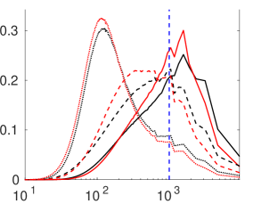
(c)

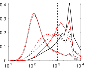
(e)

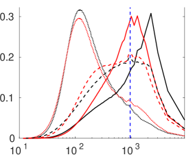
(g)

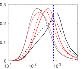
Figure 19: Premultiplied one-dimensional spanwise and streamwise spectra as function of $\lambda^{*}_{z}$ respective $\lambda^{*}_{x}$ at $Ro=0$ (a, b), $Ro=0.15$ (c, d), $Ro=0.45$ (e, f) and $Ro=0.9$ (g, h). Left column shows the spanwise spectra $k_{z}E_{K}(k_{z})$ (red lines) and $k_{z}E_{\theta\theta}(k_{z})$ (black lines). Right column shows streamwise spectra $k_{x}E_{K}(k_{x})$ (red lines) and $k_{x}E_{\theta\theta}(k_{x})$ (black lines). The spectra are at $y^{*}\approx 10$ (dotted lines), $y^{*}\approx 100$ (dashed lines) and $y\approx-0.55$ (solid lines). The vertical dashed line indicates scales with $\lambda_{x}=\lambda_{z}=1$.

At $Ro=0$, $k_{z}E_{\theta\theta}(k_{z})$ shows near the wall a peak at $\lambda^{*}_{z}\approx 100$, corresponding to the turbulent near-wall cycle, while in the outer region it has a peak at scales larger than $\lambda_{z}=h$ (figure 19.a), like the scalar spectra presented by Pirozzoli et al. (2016) for non-rotating channel flow. Also $k_{x}E_{\theta\theta}(k_{x})$ reveals large energetic scalar scales in the outer region (figure 19.b). Antonia et al. (2009) observed that the scalar variance spectra $k_{x}E_{\theta\theta}(k_{x})$ and $k_{z}E_{\theta\theta}(k_{z})$ display considerable similarities with the turbulent kinetic energy spectra $k_{x}E_{K}(k_{x})$ and $k_{z}E_{K}(k_{z})$, respectively, especially near the wall. This similarity is also reflected by the present spectra, see figure 19.(a) and (b), although the spanwise spectra indicate that away from the wall the scalar scales are somewhat wider than the turbulent scales. Overall, the scalar and turbulent length scales are thus similar in non-rotating channel flow according to the spectra. Antonia et al. (2009) found that the similarity between the spanwise spectra $k_{z}E_{\theta\theta}(k_{z})$ and $k_{z}E_{K}(k_{z})$ is mostly the consequence of a similarity between $\theta$ and streamwise velocity fluctuations $u$, whereas the streamwise scalar variance spectrum $k_{x}E_{\theta\theta}(k_{x})$ is more similar to $k_{x}E_{K}(k_{x})$, especially at larger scales, than the spectrum of the streamwise velocity component only. In the outer region, the large scales of the scalar field display in fact quite large correlations with wall-normal velocity fluctuations.

In rotating channel flow on the unstable side, $k_{x}E_{\theta\theta}(k_{x})$ and $k_{z}E_{\theta\theta}(k_{z})$ show a high similarity with $k_{x}E_{K}(k_{x})$ respective $k_{z}E_{K}(k_{z})$ near the wall at $y^{*}\approx 10$ (figure 19.c-h), although at $Ro=0.9$ the scalar scales appear somewhat shorter than the turbulence scales (figure 19.h). By contrast, away from the wall, at $y^{*}\approx 100$ and in the outer region at $y\approx-0.55$, $k_{x}E_{\theta\theta}(k_{x})$ and $k_{z}E_{\theta\theta}(k_{z})$ are more skewed towards longer and wider scales than $k_{x}E_{K}(k_{x})$ respective $k_{z}E_{K}(k_{z})$ (figure 19.c-h). This difference appears to become stronger at higher $Ro$, implying that the scalar field contains larger scales than the turbulence field in rotating channel flow. This is another demonstration of the growing difference between the scalar and turbulence field on the unstable channel side as a consequence of rotation. The sharp peaks at $\lambda_{z}=\pi h$ and $3\pi h/4$ in $k_{z}E_{\theta\theta}(k_{z})$ at $Ro=0.15$ and 0.45, respectively (figure 19.c,e) and the energetic long scales observed in $k_{x}E_{\theta\theta}(k_{x})$ at the same $Ro$ (figure 19.d,f) are most likely caused by large streamwise roll cells present at these $Ro$ (Brethouwer 2017), confirming that roll cells have a large impact on the scalar field.

The spectra at $Ro=0.15$ on the stable channel side (not shown) indicate that the scalar field is more affected by the roll cells than the turbulence field, but otherwise the turbulence and scalar scales appear similar.

IX 9. Conclusions

This paper reports a DNS study of passive scalar transport in turbulent channel flow subject to spanwise system rotation at a constant $Re=20\,000$ and $Pr=0.71$ while $Ro$ is varied from 0 to 1.2. The scalar value is constant but different at the two walls, leading to a constant mean scalar flux in the wall-normal direction in the statistically stationary state. The DNS show that rotation has a large impact on scalar transport. In rotating channel flow turbulence and turbulent scalar transport are relatively strong on the unstable channel side, whereas on the stable channel side with weak turbulence or laminar-like flow, turbulent scalar transport is weak. Although the turbulence is weaker, the scalar fluctuations are intense on the stable side or near the border between the stable and unstable channel side since the mean scalar gradient is here steep.

The main conclusions of the study are that (i) rotation weakens the similarity between the scalar and velocity field, (ii) the Reynolds analogy for scalar-momentum transfer does not hold for rotating turbulent channel flow. This is in obvious contrast to scalar transport in non-rotating turbulent channel flow where a stronger similarity between the scalar and velocity field exists and the Reynolds analogy is valid, see. e.g. Antonia et al. (2009) and Pirozzoli et al. (2016). In rotating channel flow the correlations between streamwise respective wall-normal velocity fluctuations and scalar fluctuations are weaker on the unstable respective stable channel side and the turbulent Prandtl number in the outer region of the unstable side is considerably smaller, below 0.2 at higher $Ro$, than in non-rotating channel flow. This implies that turbulent scalar transfer is very efficient on the unstable side of rotating channel flow compared to momentum transfer. Owing to rotation, the Nusselt number and the ratio of the Stanton number to skin friction both change, and the streamwise turbulent scalar flux is reduced on the unstable channel, leading to a stronger alignment between the turbulent scalar flux vector and mean scalar gradient. One-dimensional spectra of the scalar variance and turbulent kinetic energy show that the scalar scales grow relatively to the turbulence scales in the outer region of the unstable side as a result of rotation, which is another manifestation of the growing dissimilarity between velocity and scalar field. Budgets of the governing equations for the scalar variance and streamwise and wall-normal turbulent scalar fluxes are presented and discussed. These show that the Coriolis terms in the scalar flux equations reduce the streamwise and wall-normal turbulent scalar flux on the unstable and stable channel side, respectively.

Further studies of scalars in rotating shear flows are motivated given the significant effect of rotation on turbulent scalar transport and the prevalence of mass and heat transfer in rotating turbulent flows in engineering applications. However, modelling the effect of rotation on turbulent heat and mass transfer might pose a challenge since simple and convenient assumptions like the Reynolds analogy are not necessarily valid, as demonstrated by the present study.

References

- (1) Abe, H., Antonia, R.A. 2009 Near-wall similarity between velocity and scalar fluctuations in turbulent channel flow. Phys. Fluids 21, 025109.
- (2) Antonia, R.A., Abe, H., Kawamura, H. 2009 Analogy between velocity and scalar fields in a turbulent channel flow. J. Fluid Mech. 628, 241–268.
- (3) Brethouwer, G. 2005 The effect of rotation on rapidly sheared homogeneous turbulence and passive scalar transport. Linear theory and direct numerical simulations. J. Fluid Mech. 542, 305–342.
- (4) Brethouwer, G. 2016 Linear instabilities and recurring bursts of turbulence in rotating channel flow simulations. Phys. Rev. Fluids 1, 054404.
- (5) Brethouwer, G. 2017 Statistics and structure of spanwise rotating turbulent channel flow at moderate Reynolds numbers. J. Fluid Mech. 828, 424–458.
- (6) Brethouwer, G., Duguet, Y., Schlatter, P. 2012 Turbulent-laminar coexistence in wall flows with Coriolis, buoyancy or Lorentz forces. J. Fluid Mech. 704, 137–172.
- (7) Brethouwer, G., Schlatter, P., Duguet, Y., Henningson, D.H., Johansson. A.V. 2014 Recurrent bursts via linear processes in turbulent environments. Phys. Rev. Lett. 112, 144502.
- (8) Chevalier, M., Schlatter, P., Lundbladh, A. & Henningson, D. S. 2007 A pseudo-spectral solver for incompressible boundary layer flows. Technical Report TRITA-MEK 2007:07, KTH Mechanics, Stockholm, Sweden.
- (9) Dai, Y.-J., Huang, W.-X., Xu, C.-X. 2016 Effects of Taylor-Görtler vortices on turbulent flows in a spanwise-rotating channel. Phys. Fluids 28, 115104.
- (10) Deusebio, E., Brethouwer, G., Schlatter, P., Lindborg, E. 2014 A numerical study of the stratified and unstratified Ekman layer. J. Fluid Mech. 755, 672–704.
- (11) Dharmarathne, S., tutkun, M., Araya, G., Castillo, L. 2016 Structures of scalar transport in a turbulent channel. Europ. J. Mech. B/Fluids 55, 259–271.
- (12) Duguet, Y., Schlatter, P. & Henningson, D. S. 2009 Formation of turbulent patterns near the onset of transition in plane Couette flow. J. Fluid Mech. 650, 119–129.
- (13) Grundestam, O., Wallin, S., Johansson, A.V. 2008 Direct numerical simulations of rotating turbulent channel flow. J. Fluid Mech. 598, 177–199.
- (14) Hattori, H., Ohiwa, N., Kozuka, M., Nagano, Y. 2009 Improvement of the nonlinear eddy diffusivity model for rotational turbulent heat transfer at various rotating axes. Fluid Dyn. Res. 41, 012402.
- (15) Hsieh, A., Biringen, S., Kucala, A. 2016 Simulation of rotating channel flow with heat transfer: evaluation of closure models. ASME J. Turbomach. 138, 111009.
- (16) Johansson, A.V., Wikström, P.M. 1999 DNS and modelling of passive scalar transport in turbulent channel flow with a focus on scalar dissipation rate modelling. Flow Turbulence Combust. 63, 223–245.
- (17) Johnston, J.P., Halleen, R.M., Lezius, D.K. 1972 Effects of spanwise rotation on the structure of two-dimensional fully developed turbulent channel flow. J. Fluid Mech. 56, 533–559.
- (18) Kassinos, S.C., Knaepen, B., Carati, D. 2007 The transport of a passive scalar in magnetohydrodynamic turbulence subjected to mean shear and frame rotation. Phys. Fluids 19, 015105.
- (19) Kawamura, H., Abe, H., Matsuo, Y. 1999 DNS of turbulent heat transfer in channel with respect to Reynolds and Prandtl number effects. Int. J. Heat Fluid Flow 20, 196–207.
- (20) Kawamura, H., Ohsaka, K., Abe, H., Yamamoto, K. 1998 DNS of turbulent heat transfer in channel flow with low to medium-high Prandtl number fluid. Int. J. Heat Fluid Flow 19, 482–491.
- (21) Kristoffersen, R., Andersson, H.I. 1993 Direct simulations of low-Reynolds number turbulent flow in a rotating channel. J. Fluid Mech. 256, 163–197.
- (22) Lee, M., Moser, R.D. 2015 Direct numerical simulation of turbulent channel flow up to . J. Fluid Mech. 774, 395–415.
- (23) Liu, N.-S., Lu, X.-Y. 2007 Direct numerical simulation of spanwise rotating turbulent channel flow with heat transfer. Int. J. Numer. Meth. Fluids 53, 1689–1706.
- (24) Matsubara, M., Alfredsson, P.H. 1996 Experimental study of heat and momentum transfer in rotating channel flow. Phys. Fluids 8, 2964–2973.
- (25) Müller, H., Younis, B.A., Weigand, B. 2015 Development of a compact explicit algebraic model for the turbulent heat fluxes and its application in heated rotating flows. Int. J. Heat Mass Transfer 86, 880–889.
- (26) Nagano, Y., Hattori, H. 2003 Direct numerical simulation and modelling of spanwise rotating channel flow with heat transfer. J. Turbulence 4, 010.
- (27) Pirozzoli, S., Bernardini, M., Orlandi, P. 2016 Passive scalars in turbulent channel flow at high Reynolds number. J. Fluid Mech. 788, 614–639.
- (28) Wallin, S., Grundestam, O., Johansson, A.V. 2013 Laminarization mechanisms and extreme-amplitude states in rapidly rotating plane channel flow. J. Fluid Mech. 730, 193–219.
- (29) Wikström, P.M., Wallin, S., Johansson, A.V. 2000 Derivation and investigation of a new explicit algebraic model for the passive scalar flux. Phys. Fluids 12, 688–702.
- (30) Wu, H., Kasagi, N. 2004 Turbulent heat transfer in a channel with arbitrary directional system rotation. Int. J. Heat Mass Transfer 47, 4579–4591.
- (31) Xia, Z., Shi, Y., Chen, S. 2016 Direct numerical of turbulent channel flow with spanwise rotation. J. Fluid Mech. 788, 42–56.
- (32) Yang, Z., Cui, G., Xu, C., Zhang, Z. 2011 Study on the analogy between velocity and temperature fluctuations in the turbulent rotating channel flows. J. Phys.: Conf. Ser. 318, 022008.
- (33) Yang, Y.-T., Wu, J.-Z. 2012 Channel turbulence with spanwise rotation studied using helical wave decomposition. J. Fluid Mech. 692, 137–152.