Solution of linear ill-posed problems by model selection and aggregation

Abstract

We consider a general statistical linear inverse problem, where the solution is represented via a known (possibly overcomplete) dictionary that allows its sparse representation. We propose two different approaches. A model selection estimator selects a single model by minimizing the penalized empirical risk over all possible models. By contrast with direct problems, the penalty depends on the model itself rather than on its size only as for complexity penalties. A Q-aggregate estimator averages over the entire collection of estimators with properly chosen weights. Under mild conditions on the dictionary, we establish oracle inequalities both with high probability and in expectation for the two estimators. Moreover, for the latter estimator these inequalities are sharp. The proposed procedures are implemented numerically and their performance is assessed by a simulation study.

Keywords: Aggregation, ill-posed linear inverse problems, model selection, oracle inequality, overcomplete dictionary
AMS (2000) Subject Classification: Primary: 62G05. Secondary: 62C10

1 Introduction

Linear inverse problems, where the data is available not on the object of primary interest but only in the form of its linear transform, appear in a variety of fields: medical imaging (X-ray tomography, CT and MRI), astronomy (blured images), finance (model calibration of volatility) to mention just a few. The main difficulty in solving inverse problems is due to the fact that most of practically interesting and relevant cases fall into into the category of so-called ill-posed problems, where the solution cannot be obtained numerically by simple invertion of the transform. In statistical inverse problems the data is, in addition, corrupted by random noise that makes the solution even more challenging.

Statistical linear inverse problems have been intensively studied and there exists an enormous amount of literature devoted to various theoretical and applied aspects of their solutions. We refer a reader to to Cavalier (2009) for review and references therein.

Let $\cal G$ and $\cal H$ be two separable Hilbert spaces and $A:\cal G\rightarrow\cal H$ be a bounded linear operator. Consider a general statistical linear inverse problem

$$y=Af+\sigma\varepsilon,$$ (1)

where $y$ is the observation, $f\in G$ is the (unknown) object of interest, $\varepsilon$ is a white noise and $\sigma$ is a (known) noise level. For ill-posed problems $A^{-1}$ does not exist as a linear bounded operator.

Most of approaches for solving (1) essentially rely on reduction of the original problem to a sequence model using the following general scheme:

1. Choose some orthonormal basis $\{\phi_{j}\}$ on $\cal G$ and expand the unknown $f$ in (1) as

   $$f=\sum_{j}\langle f,\phi_{j}\rangle_{G}~{}\phi_{j}$$ (2)

2. Define $\psi_{j}$ as the solution of $A^{*}\psi_{j}=\phi_{j}$, where $A^{*}$ is the adjoint operator, that is, $\psi_{j}=A(A^{*}A)^{-1}\phi_{j}$. Reduce (1) to the equivalent sequence model:

   $$\langle y,\psi_{j}\rangle_{H}~{}=~{}\langle Af,\psi_{j}\rangle_{H}+\langle\varepsilon,\psi_{j}\rangle_{H}~{}=~{}\langle f,\phi_{j}\rangle_{G}+\langle\varepsilon,\psi_{j}\rangle_{H},$$ (3)

   where for ill-posed problems $\mbox{Var}\left(\langle y,\psi_{j}\rangle_{H}\right)=\sigma^{2}\|\psi_{j}\|_{H}^{2}$ increases with $j$. Following the common terminology, an inverse problem is called mildly ill-posed, if the variances increase polynomially and severely ill-posed if their growth is exponential (see, e.g., Cavalier, 2009).

3. Estimate the unknown coefficients $\langle f,\phi_{j}\rangle_{G}$ from empirical coefficients $\langle y,\psi_{j}\rangle_{H}$: $\widehat{\langle f,\phi_{j}\rangle_{G}}=\delta\{\langle y,\psi_{j}\rangle_{H}\}$, where $\delta(\cdot)$ is some truncating/shrinking/thresholding procedure (see, e.g., Cavalier 2009, Section 1.2.2.2 for a survey), and reconstruct $f$ as

   $$\hat{f}=\sum_{j}\widehat{\langle f,\phi_{j}\rangle_{G}}~{}\phi_{j}$$

Efficient representation of $f$ in a chosen basis $\{\phi_{j}\}$ in (2) is essential. In the widely-used singular value decomposition (SVD), $\phi_{j}$’s are the orthogonal eigenfunctions of the self-adjoint operator $A^{*}A$ and $\psi_{j}=\lambda_{j}^{-1}A\phi_{j}$, where $\lambda_{j}$ is the corresponding eigenvalue. SVD estimators are known to be optimal in various minimax settings over certain classes of functions (e.g., Johnstone & Silverman, 1990; Cavalier & Tsybakov, 2002; Cavalier et al., 2002). A serious drawback of SVD is that the basis is defined entirely by the operator $A$ and ignores the specific properties of the object of interest $f\in\cal G$. Thus, for a given $A$, the same basis will be used regardless of the nature of a scientific problem at hand. While the SVD-basis could be very efficient for representing $f$ in one area, it might yield poor approximation in the other. The use of SVD, therefore, restricts one within certain classes $\cal G$ depending on a specific operator $A$. See Donoho (1995) for further discussion.

In wavelet-vaguelette decomposition (WVD), $\phi_{j}$’s are orthonormal wavelet series. Unlike SVD-basis, wavelets allows sparse representation for various classes of functions and the resulting WVD estimators have been studied in Donoho (1995), Abramovich & Silverman (1998), Kalifa & Mallat (2003), Johnstone et al. (2004). However, WVD imposes relatively stringent conditions on $A$ that are satisfied only for specific types of operators, mainly of convolution type.

A general shortcoming of orthonormal bases is due to the fact that they may be “too coarse” for efficient representation of unknown $f$. Since 90s, there was a growing interest in the atomic decomposition of functions over overcomplete dictionaries (see, for example, Mallat & Zhang, 1993; Chen, Donoho & Saunders, 1999; Donoho & Elad, 2003). Every basis is essentially only a minimal necessary dictionary. Such “miserly” representation usually causes poor adaptivity (Mallat & Zhang, 1993). Application of overcomplete dictionaries improves adaptivity of the representation, because one can choose now the most efficient (sparse) one among many available. One can see here an interesting analogy with colors. Theoretically, every other color can be generated by combining three basic colors (green, red and blue) in corresponding proportions. However, a painter would definitely prefer to use the whole available palette (overcomplete dictionary) to get the hues he needs! Selection of appropriate subset of atoms (model selection) that allows a sparse representation of a solution is a core element in such an approach. Pensky (2016) was probably the first to use overcomplete dictionaries for solving inverse problems. She utilized the Lasso techniques for model selection within the overcomplete dictionary, established oracle inequalities with high probability and applied the proposed procedure to several examples of linear inverse problems. However, as usual with Lasso, it required somewhat restrictive compatibility conditions on the design matrix $\Phi$.

In this paper we propose two alternative approaches for overcomplete dictionaries based estimation in linear ill-posed problems. The first estimator is obtained by minimizing penalized empirical risk with a penalty on model $M$ proportional to $\sum_{j\in M}\|\psi_{j}^{2}\|$. The second one is based on a Q-aggregation type procedure that is specifically designed for solution of linear ill-posed problems and is different from that of Dai et al. (2012) developed for solution of direct problems. We establish oracle inequalities for both estimators that hold with high probabilities and in expectation. Moreover, for the Q-aggregation estimator, the inequalities are sharp. Simulation study shows that the new techniques produce more accurate estimators than Lasso.

The rest of the paper is organized as follows. Section 2 introduces the notations and some preliminary results. The model selection and aggregation-type procedures are studied respectively in Section 3 and Section 4. The simulation study is described in Section 5. All proofs are given in the Appendix.

2 Setup and notations

Consider a discrete analog of a general statistical linear inverse problem (1):

$$y=Af+\sigma\varepsilon,$$ (4)

where $y\in\mathbb{R}^{n}$ is the vector of observations, $f\in\mathbb{R}^{n}$ is the unknown vector to be recovered, $A$ is a known (ill-posed) $n\times m\;(n\geq m)$ matrix with $rank(A)=m$, and $\varepsilon\sim N(0,I_{n})$.

In what follows $\|\cdot\|$ and $\langle\cdot,\cdot\rangle$ denote respectively a Euclidean norm and an inner product in $\mathbb{R}^{n}$. Let $\phi_{j}\in\mathbb{R}^{n},\;j=1,\cdots,p$ with $\|\phi_{j}\|=1$ be a set of normalized vectors (dictionary), where typically $p>n$ (overcomplete dictionary). Let $\Phi_{n\times p}$ be the complete dictionary matrix with the columns $\phi_{j},\;j=1,\ldots,p$, and $\Psi_{n\times p}$ is such that $A^{T}\Psi=\Phi$, that is, $\Psi=A(A^{T}A)^{-1}\Phi$ and $\psi_{j}=A(A^{T}A)^{-1}\phi_{j}$.

In what follows, we assume that, for some positive $r$, the minimal $r$-sparse eigenvalue of $\Phi^{T}\Phi$ is separated from zero:

$$\nu^{2}_{r}=\min_{x\in\mathbb{R}^{n},\|x\|_{0}\leq r}\frac{\|\Phi x\|^{2}}{\|x\|^{2}}>0$$

and consider a set of models ${\cal M}=\{M\subseteq\{1,\ldots,p\}:|M|\leq r/2\}$ of sizes not larger than $r/2$.

For a given model $M\subseteq\{1,\ldots,p\}$ define a $p\times p$ diagonal indicator matrix $D_{M}$ with diagonal entries $d_{Mj}=I\{j\in M\}$. The design matrix corresponding to $M$ is then $\Phi_{M}=\Phi D_{M}$, while $\Psi_{M}=\Psi D_{M}=A(A^{T}A)^{-1}\Phi_{M}$. Let $H_{M}=\Phi_{M}(\Phi_{M}^{T}\Phi_{M})^{-1}\Phi_{M}^{T}$ be the projection matrix on a span of nonzero columns of $\Phi_{M}$ and

$$f_{M}=H_{M}f=\Phi_{M}(\Phi_{M}^{T}\Phi_{M})^{-1}\Phi_{M}^{T}~{}f=\Phi_{M}(\Phi_{M}^{T}\Phi_{M})^{-1}\Psi_{M}^{T}~{}Af$$

be the projection of $f$ on $M$. Denote

$$z=(A^{T}A)^{-1}A^{T}y=f+\xi,\;{\rm where}\;\xi=(A^{T}A)^{-1}A^{T}\varepsilon.$$ (5)

Consider the corresponding projection estimator

$$\hat{f}_{M}=H_{M}z=H_{M}(A^{T}A)^{-1}A^{T}y=\Phi_{M}(\Phi_{M}^{T}\Phi_{M})^{-1}\Psi_{M}^{T}~{}y=\Phi_{M}\hat{\theta}_{M},$$ (6)

where the vector of projection coefficients $\hat{\theta}_{M}=(\Phi_{M}^{T}\Phi_{M})^{-1}\Psi_{M}^{T}~{}y$. By straightforward calculus, $\hat{f}_{M}\sim N(f_{M},\sigma^{2}H_{M}(A^{T}A)^{-1}H_{M})$ and the quadratic risk

$$E\|\hat{f}_{M}-f\|^{2}=\|f_{M}-f\|^{2}+\sigma^{2}\mbox{Tr}\left((A^{T}A)^{-1}H_{M}\right)$$ (7)

The oracle model is the one that minimizes (7) over all models $M\in{\cal M}$ and the ideal oracle risk is

$$R({\rm oracle})=\inf_{M\in{\cal M}}E\|\hat{f}_{M}-f\|^{2}=\inf_{M}\left\{\|f_{M}-f\|^{2}+\sigma^{2}\mbox{Tr}\left((A^{T}A)^{-1}H_{M}\right)\right\}$$ (8)

The oracle risk is obviously unachievable but can be used as a benchmark for a quadratic risk of any available estimator.

3 Model selection by penalized empirical risk

For a given model $M\in{\cal M}$, $\hat{f}_{M}$ in (6) minimizes the corresponding empirical risk $\|z-\tilde{f}_{M}\|^{2}$, where $z$ was defined in (5). Select a model $\widehat{M}$ by minimizing the penalized empirical risk:

$$\widehat{M}=\underset{M\in{\cal M}}{\operatorname{argmin}}\,\left\{\|z-\hat{f}_{M}\|^{2}+\mbox{Pen}(M)\right\}=\underset{M\in{\cal M}}{\operatorname{argmin}}\,\left\{-\|\hat{f}_{M}\|^{2}+\mbox{Pen}(M)\right\},$$ (9)

where $\mbox{Pen}(M)$ is a penalty function on a model $M$. The proper choice of $\mbox{Pen}(M)$ is the core of such an approach.

For direct problems ($A=I$), the penalized empirical risk approach, with the complexity type penalties $\mbox{Pen}(|M|)$ on a model size, has been intensively studied in the literature. In the last decade, in the context of linear regression, the in-depth theories (risk bounds, oracle inequalities, minimaxity) have been developed by a number of authors (see, e.g., Foster & George (1994), Birgé & Massart (2001, 2007), Abramovich & Grinshtein (2010), Rigollet & Tsybakov (2011), Verzelen (2012) among many others).

For inverse problems, Cavalier et al. (2002) considered a truncated orthonormal series estimator, where the cut-off point was chosen by SURE criterion corresponding to the AIC-type penalty $\mbox{Pen}(M)=2\sigma^{2}\mbox{Tr}((A^{T}A)^{-1}H_{M})$ and established oracle inequalities for the resulting estimator $\hat{f}_{\widehat{M}}$. It was further generalized and improved by risk hull minimization in Cavalier & Golubev (2006).

To the best of our knowledge, Pensky (2016) was the first to consider model selections within overcomplete dictionaries by empirical risk minimization for statistical inverse problems. She utilized Lasso penalty. However, as usual with Lasso, it required somewhat restrictive compatibility conditions on the design matrix $\Phi$ (see Pensky, 2016 for more details).

In this paper, we utilize the penalty $\mbox{Pen}(M)$ that depends on the Frobenius norm of the matrix $\Psi_{M}$:

$$\|\Psi_{M}\|^{2}_{F}=\sum_{j\in M}\|\psi_{j}\|^{2}=\mbox{Tr}\left((A^{T}A)^{-1}\Phi_{M}\Phi_{M}^{T}\right)$$

The following theorem provides nonasymptotic upper bounds for the quadratic risk of the resulting estimator $\hat{f}_{\widehat{M}}$ both with high probability and in expectation:

Theorem 1.

Consider the model (4) and the penalized empirical risk estimator $\hat{f}_{\widehat{M}}$, where the model ${\widehat{M}}$ is selected w.r.t. (9) with the penalty

$$\mbox{Pen}(M)\geq\frac{4\sigma^{2}(\delta+1)}{a\nu^{2}_{r}}\ \|\Psi_{M}\|^{2}_{F}\ \ln p$$ (10)

for some $\delta>0$ and $0<a<1$. Then,

1. With probability at least $1-\sqrt{\frac{2}{\pi}}~{}p^{-\delta}$

   $$\|\hat{f}_{\widehat{M}}-f\|^{2}\leq\frac{1+a}{1-a}~{}\min_{M\in{\cal M}}\left\{\|f_{M}-f\|^{2}+\frac{a^{2}+a+4}{2(1+a)}~{}\mbox{Pen}(M)\right\}$$ (11)

2. If, in addition, we restrict the set of admissible models to ${\cal M}_{\gamma}=\{M\in{\cal M}:\|\Psi_{M}\|_{F}^{2}\leq\gamma^{2}n\}$ for some constant $\gamma$,

   $$E\|\hat{f}_{\widehat{M}}-f\|^{2}\leq\frac{1+a}{1-a}~{}\min_{M\in{\cal M}_{\gamma}}\left\{\|f_{M}-f\|^{2}+\frac{3}{2(1+a)}~{}\mbox{Pen}(M)\right\}+\frac{4\gamma^{2}\sigma^{2}}{a(1-a)\nu^{2}_{r}}~{}np^{-\delta}$$ (12)

The additional restriction on the set of models ${\cal M}$ in the second part of Theorem 1 is required to guarantee that the oracle risk in (8) does not grow faster than $n$.

Note that for the direct problems, $\Psi_{M}=\Phi_{M}$ and the penalty (10) is the RIC-type complexity penalty of Foster & George (1994) of the form $\mbox{Pen}(M)=C|M|\ln p$.

We can compare the quadratic risk of the proposed estimator with the oracle risk $R({\rm oracle})$ in (8). Consider the penalty

$$\mbox{Pen}(M)=\frac{4\sigma^{2}(\delta+1)}{a\nu^{2}_{r}}\ \|\Psi_{M}\|^{2}_{F}\ \ln p$$ (13)

for some $0<a<1$ and $\delta\geq 2$. Assume that $p\geq n$ (overcomplete dictionary) and choose $\delta\geq 2$. Then, the last term in the RHS of (12) turns to be of a smaller order and we obtain

$$E\|\hat{f}_{\widehat{M}}-f\|^{2}\leq C_{1}\min_{M\in{\cal M}_{\gamma}}\left\{\|f_{M}-f\|^{2}+C_{2}\frac{\gamma\sigma^{2}}{\nu_{r}^{2}}\|\Psi_{M}\|^{2}_{F}\ln p\right\}$$

for some positive constants $C_{1},C_{2}$ depending on $a$ and $\delta$ only. By standard linear algebra arguments, $\|\Psi_{M}\|^{2}_{F}=\mbox{Tr}\left((A^{T}A)^{-1}\Phi_{M}\Phi_{M}^{T}\right)\leq\kappa^{2}_{r}~{}\mbox{Tr}\left((A^{T}A)^{-1}H_{M}\right)$ and, therefore, the following oracle inequality holds:

Corollary 1.

Assume that $p\geq n$ and consider the penalized empirical risk estimator ${\widehat{M}}$ from Theorem 1, where ${\widehat{M}}$ is selected w.r.t. (9) over ${\cal M}_{\gamma}$ with the penalty (13) for some $0<a<1$ and $\delta\geq 2$. Then,

$$E\|\hat{f}_{\widehat{M}}-f\|^{2}\leq C_{0}\frac{\kappa^{2}_{r}}{\nu^{2}_{r}}\ln p~{}R({\rm oracle})$$

for some constant $C_{0}>0$ depending on $a$, $\delta$ and $\gamma$ only.

Thus, the quadratic risk of the proposed estimator $\hat{f}_{\widehat{M}}$ is within $\ln p$-factor of the ideal oracle risk. The $\ln p$-factor is a common closest rate at which an estimator can approach an oracle even in direct (complete) model selection problems (see, e.g., Donoho & Johnstone, 1994; Birgé & Massart, 2001; Abramovich & Grinshtein, 2010; Rigollet & Tsybakov, 2011; and also Pensky (2016) for inverse problems). For an ordered model selection within a set of nested models, it is possible to construct estimators that achieve the oracle risk within a constant factor (see, e.g., Cavalier et al., 2002 and Cavalier & Golubev, 2006).

Similar oracle inequalities (even sharp with the coefficient in front of $\|f_{M}-f\|^{2}$ equals to one) with high probability were obtained for the Lasso estimator but under the additional compatibility assumption on the matrix $\Phi$ (Pensky, 2016).

4 Q-aggregation

Note that inequalities (11) and (12) in Theorem 1 for model selection estimator are not sharp in the sense that the coefficient in front of the minimum is greater than one. In order to derive sharp oracle inequalities both in probability and expectation, one needs to aggregate the entire collection of estimators: $\hat{f}=\sum_{M\in{\cal M}}\theta_{M}\hat{f}_{M}$ rather than to select a single estimator $\hat{f}_{\widehat{M}}$.

Leung & Barron (2006) considered exponentially weighted aggregation (EWA) with $\theta_{M}\propto\pi_{M}\exp\{\|z-\hat{f}_{M}\|^{2}/\beta\}$, where $\pi$ is some (prior) probability measure on ${\cal M}$ and $\beta>0$ is a tuning parameter. They established sharp oracle inequalities in expectation for EWA in direct problems. Dalalyan & Salmon (2012) proved sharp oracle inequalities in expectation for EWA of affine estimators in nonparametric regression model. Their paper offers limited extension of the theory to the case of mildly ill-posed inverse problems where $\mbox{Var}(\langle y,\psi\rangle_{H})=\sigma^{2}\|\psi_{j}\|^{2}_{H}$ increase at most polynomially with $j$. However, their results are valid only for the SVD decomposition and require block design which seriously limits the scope of application of their theory. Moreover, Dai et al. (2012) argued that EWA cannot satisfy sharp oracle inequalities with high probability and proposed instead to use Q-aggregation.

Define a general Q-aggregation estimator of $f$ as

$$\hat{f}_{\hat{\theta}}=\sum_{M\in{\cal M}}\theta_{M}\hat{f}_{M},$$ (14)

where the vector of weights $\hat{\theta}$ is the solution of the following optimization problem:

$$\hat{\theta}=\underset{\theta\in\Theta_{{\cal M}}}{\operatorname{argmin}}\,\left\{\alpha\sum_{M\in{\cal M}}\theta_{M}\|z-\hat{f}_{M}\|^{2}+(1-\alpha)\Big{\|}z-\sum_{M\in{\cal M}}\theta_{M}\hat{f}_{M}\Big{\|}^{2}+\mbox{Pen}(\theta)\right\}$$ (15)

for some $0\leq\alpha\leq 1$ and a penalty $\mbox{Pen}(\theta)$, and $\Theta_{{\cal M}}$ is the simplex

$$\Theta_{{\cal M}}=\{\theta\in\mathbb{R}^{card({\cal M})}:\theta_{M}\geq 0,\;\sum_{M\in{\cal M}}\theta_{M}=1\}$$ (16)

In particular, Dai et al. (2012) considered $\mbox{Pen}(\theta)$ proportional to the Kullback-Leibler divergence $KL(\theta,\pi)$ for some prior $\pi$ on $\Theta_{{\cal M}}$. For direct problems, they derived sharp oracle inequalities both in expectation and with high probability for Q-aggregation with such penalty. In fact, EWA can also be viewed as an extreme case of Q-aggregation of Dai et al. for $\alpha=1$ (see Rigolette & Tsybakov, 2012). However, the results for Q-aggregation with Kullback-Leibler-type penalty are not valid for ill-posed problems.

In this section we propose a different type of penalty for Q-aggregation in (15) that is specifically designed for the solution of inverse problems. In particular, this penalty allows one to obtain sharp oracle inequalities both in expectation and with high probability in both mild and severe ill-posed linear inverse problems. Namely, we consider the penalty

$$\mbox{Pen}(\theta)=\frac{4\sigma^{2}\,(\delta+1)\ln p}{\nu^{2}_{r}}\sum_{M\in{\cal M}}\theta_{M}\|\Psi_{M}\|^{2}_{F}$$ (17)

with a tuning parameter $\delta>0$. For such a penalty and $\alpha=1/2$, the resulting $\hat{\theta}$ is

$$\hat{\theta}=\underset{\theta\in\Theta_{{\cal M}}}{\operatorname{argmin}}\,\left\{\sum_{M\in{\cal M}}\theta_{M}\left(\|z-\hat{f}_{M}\|^{2}+\frac{8\sigma^{2}\,(\delta+1)\ln p}{\nu^{2}_{r}}\,\|\Psi_{M}\|^{2}_{F}\right)+\Big{\|}z-\sum_{M\in{\cal M}}\theta_{M}\hat{f}_{M}\Big{\|}^{2}\right\}$$ (18)

Note that the first term in the minimization criteria (18) is the same as in model selection (9) with the penalty (10) for $a=1/2$. The presence of the second term is inherent for Q-aggregation. In fact, the model selection estimator $\hat{f}_{\widehat{M}}$ from Section 3 is a particular case of a Q-aggregate estimator $\hat{f}_{\hat{\theta}}$ with the weights obtained by solution of problem (15) with $\alpha=1$.

The non-asymptotic upper bounds for the quadratic risk of $\hat{f}_{\hat{\theta}}$, both with high probability and in expectation, are given by the following theorem :

Theorem 2.

Consider the model (4) and the Q-aggregate estimator $\hat{f}_{\theta}$ given by (14), where the weights ${\theta}$ are selected as a solution of the optimization problem (18). Then,

1. With probability at least $1-\sqrt{\frac{2}{\pi}}~{}p^{-\delta}$

   $$\|\hat{f}_{\hat{\theta}}-f\|^{2}\leq\min_{M\in{\cal M}}\left\{\|f_{M}-f\|^{2}+10\nu^{-2}_{r}\,\sigma^{2}(\delta+1)\ \|\Psi_{M}\|^{2}_{F}\ \ln p\right\}$$ (19)

2. If, in addition, we restrict the set of admissible models to ${\cal M}_{\gamma}=\{M\in{\cal M}:\|\Psi_{M}\|_{F}^{2}\leq\gamma^{2}n\}$ for some constant $\gamma$, then

   $$E\|\hat{f}_{\widehat{M}}-f\|^{2}\leq\min_{M\in{\cal M}_{\gamma}}\left\{\|f_{M}-f\|^{2}+\nu^{-2}_{r}\,\sigma^{2}\|\Psi_{M}\|^{2}_{F}\,\left(3+2(\delta+1)\,\ln p\right)\right\}+2\gamma^{2}\,np^{-\delta}$$ (20)

Observe that unlike Theorem 1 for model selection estimator, inequalities in both (19) and (20) for Q-aggregation are sharp.

5 Simulation study

In this section we present results of a simulation study that illustrates the performance of the model selection estimator ${\widehat{M}}$ from (9) with the penalty (10) and the Q-aggregation estimator $\hat{f}_{\hat{\theta}}$ given by (14) where the weights are defined in (18).

The data were generated w.r.t. a (discrete) ill-posed statistical linear problem (4) corresponding to the convolution-type operator $Af(t)=\int_{0}^{t}e^{-(t-x)}f(x)dx,\;0\leq t\leq 1$, on a regular grid $t_{i}=i/n$:

$$A_{ij}=e^{-\frac{i-j}{n}}\,I(j\leq i),\;\;\;i,j=1,\ldots,n,$$

where $I(\cdot)$ is the indicator function and $n=128$.

We considered the dictionary obtained by combining two wavelet bases of different type: the Daubechies 8 wavelet basis $\{\phi^{D}_{3,0},...,\psi^{D}_{3,0},...,\psi^{D}_{6,63}\}$ and the Haar basis $\{\phi^{H}_{3,0},...,\psi^{H}_{3,0},...,\psi^{H}_{5,53}\}$, with the overall dictionary size $p=128+64=192$. In our notations, $\phi^{D}$ and $\phi^{H}$ are the scaling functions, while $\psi^{D}$ and $\psi^{H}$ are the wavelets functions of the Daubechies and Haar bases respectively with the initial resolution level $J_{0}=3$.

In order to investigate the behavior of the estimators, we considered various sparsity and noise levels. In particular, we used four test functions, presented in Figure 2, that correspond to different sparsity scenarios:

1. $f_{1}=\phi^{D}_{3,4}+\phi^{H}_{3,0}$ (high sparsity)

2. $f_{2}=\phi^{D}_{3,0}+\phi^{D}_{3,6}+\psi^{D}_{3,7}+\phi^{H}_{3,6}$ (moderate sparsity)

3. $f_{3}=\phi^{D}_{3,1}+\phi^{D}_{3,5}+\phi^{D}_{3,7}+\psi^{D}_{3,0}+\psi^{D}_{3,3}+\psi^{D}_{3,5}+\phi^{H}_{3,0}+\phi^{H}_{3,3}$ (low sparsity)

4. $f_{4}$ is the well-known HeaviSine function from Donoho & Johnstone (1994) (uncontrolled sparsity)

For each test function, we used three different values of $\sigma$ that were chosen to ensure a signal-to-noise ratios $SNR=10,7,5$, where $SNR(f)=\|f\|/\sigma$.

The accuracy of each estimator was measured by its relative integrated error:

$$R(\hat{f})=\|f-\hat{f}\|^{2}/\|f\|^{2}$$

Since the model selection estimator $\hat{f}_{\widehat{M}}$ involves minimizing a cost function of the form $-\|\hat{f}_{M}\|^{2}+4\sigma^{2}\lambda\ln p\|\Psi_{M}\|^{2}_{F}$ over the entire model space ${\cal M}$ of a very large size, we used a Simulated Annealing (SA) stochastic optimization algorithm for an approximate solution. The SA algorithm is a kind of a Metropolis sampler where the acceptance probability is “cooled down” by a synthetic temperature parameter (see Brémaud 1999, Chapter 7, Section 8). More precisely, if $M^{(r)}$ is a solution at step $r>0$ of the algorithm, at step $r+1$ a tentative solution $M^{*}$ is selected according to a given symmetric proposal distribution and it is accepted with probability

$$a(M^{*},M^{(r)})=\min\left\{1,\exp\left(-\frac{\pi(M^{*})-\pi(M^{(r)})}{T^{(r)}}\right)\right\}.$$ (21)

where $T^{(r)}$ is a temperature parameter at step $r$. The expression (21) is motivated by the fact that while $M^{*}$ is always accepted if $\pi(M^{(r)})\geq\pi(M^{*})$, it can still be accepted even if $\pi(M^{(r)})<\pi(M^{*})$ in spite of being worse than the current one. The chance of acceptance of $M^{*}$ for the same value of $\pi(M^{(r)})-\pi(M^{*})<0$ diminishes at every step as the temperature $T^{(r)}$ decreases with $r$. The law that reduces the temperature is called the cooling schedule, in particular, here we choose $T^{(r)}=1/(1+\log(r))$.

In this paper we adopted the classical symmetric uniform proposal distribution and selected a starting solution $M^{(0)}$ according to the following initial probability

$$p(j)=C\exp\{\langle\psi_{j},y\rangle^{2}-c\|\psi_{j}\|^{2}\},\quad\mbox{for }j=1,\ldots,p$$ (22)

where $c=\sum_{j}\langle\psi_{j},y\rangle^{2}/\sum_{j}\|\psi_{j}\|^{2}$ and $C=\left[\sum_{j=1}^{p}\exp\{\langle\psi_{j},y\rangle^{2}-c\|\psi_{j}\|^{2}\}\right]^{-1}$ is the normalizing constant. Observe that the argument in the exponent in (22) is the difference of $\langle\psi_{j},y\rangle^{2}$ and $\|\psi_{j}\|^{2}$ where the first term $\langle\psi_{j},y\rangle^{2}$ is the squared $j$-th empirical coefficient while the second term $\|\psi_{j}\|^{2}$ is the increase in the variance due to the addition of the $j$-th dictionary function. Hence, the prior $p(j)$ is more likely to choose dictionary functions with small variances that are highly correlated to the true function $f$.

Thus, the adopted SA procedure can be summarized as follows:

• generate a random number $m\leq n/\log(p)$. Set $T^{(1)}=1$

• generate a starting solution $M^{(0)}$ with $\mbox{card}(M^{(0)})=m$ by sampling indices $j\in\{1,\ldots,p\}$ according to the probability given by equation (22)

• repeat for $r=1,2,...r_{max}$

  1. generate a variable $j^{*}\sim\ \mbox{Uniform}\,(1,...,p)$

  2. if $j^{*}\notin M^{(r)}$ propose $M^{*}=M^{(r)}\cup\{j^{*}\}$

     else

     propose $M^{*}=M^{(r)}-\{j^{*}\}$

  3. with probability $a(M^{*},M^{(r)})$ given in equation (21) assign $M^{(r+1)}=M^{*}$, otherwise $M^{(r+1)}=M^{(r)}$

  4. update the temperature parameter $T^{(r+1)}=1/(1+\log(r+1))$

While various stopping criteria could be used in the SA procedure, we found $r_{max}=100,000$ to be sufficient for obtaining a good approximation of the global minimum in (9). Once the algorithm is terminated, we evaluated $\hat{f}_{\widehat{M}}$, where $\widehat{M}=\arg\min_{0\leq r\leq r_{max}}\pi(M^{(r)})$ was the “best” model in the chain of models generated by SA algorithm.

Similarly, the Q-aggregation estimator $\hat{f}_{\hat{\theta}}$ involves computationally expensive aggregation of estimators over the entire model space ${\cal M}$. We, therefore, approximated it by aggregating over the subset ${\cal M}^{{}^{\prime}}$ of the last 50 “visited” models in the SA chain, i.e. $\hat{f}_{\hat{\theta}}=\sum_{M\in{\cal M}^{{}^{\prime}}}\hat{\theta}_{M}\hat{f}_{M}$ with $\hat{\theta}$ being a solution of (18).

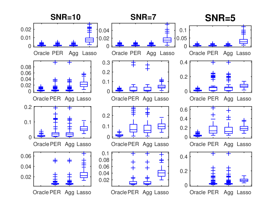
Figure 1: The boxplots of the relative integrated errors of $\hat{f}_{oracle}$, $\hat{f}_{\widehat{M}}$, $\hat{f}_{\theta}$ and $\hat{f}_{Lasso}$ over 100 independent runs. Top row: $f_{1}$, second row: $f_{2}$, third row $f_{3}$, bottom row $f_{4}$.

For $f_{1}$, $f_{2}$ and $f_{3}$ we also considered the oracle projection estimator $\hat{f}_{oracle}$ based on the true model. In addition, we compared the proposed estimators with the Lasso-based estimator $\hat{f}_{Lasso}=\sum_{j=1}^{p}\hat{\theta}_{j}\phi_{j}$ of Pensky (2016), where the vector of coefficients $\hat{\theta}$ is a solution of the following optimization problem

$$\hat{\theta}=\arg\min_{\theta}\left\{\left\|\sum_{j=1}^{p}\theta_{j}\phi_{j}\right\|^{2}-2\sum_{j=1}^{p}\theta_{j}\langle y,\psi_{j}\rangle+\lambda\sum_{j=1}^{p}|\theta_{j}|\,\|\psi_{j}\|^{2}\right\},$$

and $\lambda$ is a tuning parameter.

The tuning parameters $\lambda$ for $\hat{f}_{\widehat{M}}$ and $\hat{f}_{Lasso}$, were chosen by minimizing the error on a grid of possible values. To reduce heavy computational costs we used the same $\lambda$ of $\hat{f}_{\widehat{M}}$ for all 50 aggregated models used for calculating $\hat{f}_{\hat{\theta}}$.

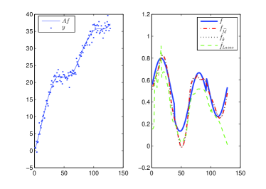
Figure 2: The test functions, observed data and estimators for $SNR=5$. In each block of figures corresponding to four test functions, the left panel shows the data $y$ and the true $Af$; the right panel shows the true $f$ and the four estimators. Top left: $f_{1}$; top right: $f_{2}$; bottom left: $f_{3}$; bottom right: $f_{4}$.

Figure 1 presents the boxplots of $R(\hat{f})$ over 100 independent runs for $\hat{f}_{oracle}$ (for $f_{1},f_{2}$ and $f_{3}$), $\hat{f}_{\widehat{M}}$, $\hat{f}_{\hat{\theta}}$ and $\hat{f}_{Lasso}$. Performances of all estimators deteriorate as SNR decreases especially for the less sparse test functions. The estimators $\hat{f}_{\widehat{M}}$ and $\hat{f}_{\hat{\theta}}$ always outperform $\hat{f}_{Lasso}$ and, as it is expected from our theoretical statements, $\hat{f}_{\hat{\theta}}$ yields somewhat better results than $\hat{f}_{\widehat{M}}$. We expect that the differences in precisions of $\hat{f}_{\widehat{M}}$ and $\hat{f}_{\hat{\theta}}$ would be more significant if we carried out aggregation over a larger portion of the model space than the last 50 visited models. Figure 2 illustrates these conclusion by displaying examples of the estimators for $SNR=5$. We should also mention that estimator $\hat{f}_{\widehat{M}}$ was usually more sparse than $\hat{f}_{Lasso}$.

Appendix

The proofs of the main results are based on the following auxiliary lemmas.

Lemma 1.

For any $x>0$,

$$P\left(\sup_{M\in{\cal M}}\left\{\|\Psi_{M}^{T}\varepsilon\|^{2}-2\sigma^{2}\|\Psi_{M}\|^{2}_{F}(\ln p+x)\right\}\leq 0\right)\geq 1-{\sqrt{\frac{2}{\pi}}}~{}e^{-x}$$

Proof.

For any model $M\in{\cal M}$, $\|\Psi_{M}^{T}\varepsilon\|^{2}=\sum_{j\in M}(\psi_{j}^{T}\varepsilon)^{2}$, where $\psi_{j}^{T}\varepsilon\sim N(0,\sigma^{2}\|\psi_{j}\|^{2})$. By Mill’s ratio

$$P\left((\psi_{j}^{T}\varepsilon)^{2}>2\sigma^{2}\|\psi_{j}\|^{2}(\ln p+x)\right)\leq{\sqrt{\frac{2}{\pi}}}~{}p^{-1}e^{-x}$$

for any $x>0$. Then,

$$\begin{split}P&\left(\bigcap_{j\in M}\left\{(\psi_{j}^{T}\varepsilon)^{2}-2\sigma^{2}\|\psi_{j}\|^{2}(\ln p+x)\leq 0\right\}\right)\geq 1-\sum_{j\in{\cal M}}P\left((\psi_{j}^{T}\varepsilon)^{2}-2\sigma^{2}\ \|\psi_{j}\|^{2}(\ln p+x)>0\right)\\ &\geq 1-{\sqrt{\frac{2}{\pi}}}~{}e^{-x}\end{split}$$

and, therefore,

$$\begin{split}P&\left(\sup_{M\in{\cal M}}\left\{\|\Psi_{M}^{T}\varepsilon\|^{2}-2\sigma^{2}\|\Psi_{M}\|^{2}_{F}(\ln p+x)\leq 0\right\}\right)\geq P\left(\bigcap_{M\in{\cal M}}\bigcap_{j\in M}\left\{(\psi_{j}^{T}\varepsilon)^{2}-2\sigma^{2}\ \|\psi_{j}\|^{2}(\ln p+x)\leq 0\right\}\right)\\ &=P\left(\bigcap_{j=1}^{p}\left\{(\psi_{j}^{T}\varepsilon)^{2}-2\sigma^{2}\ \|\psi_{j}\|^{2}(\ln p+x)\leq 0\right\}\right)\geq 1-{\sqrt{\frac{2}{\pi}}}~{}p^{-1}e^{-x}\end{split}$$

∎

Lemma 2.

For any $M_{1},M_{2}\in{\cal M}$, one has

$$\mbox{Tr}(\Psi_{M_{1}\cup M_{2}}^{T}\Psi_{M_{1}\cup M_{2}}) \leq \mbox{Tr}(\Psi_{M_{1}}^{T}\Psi_{M_{1}})+\mbox{Tr}(\Psi_{M_{2}}^{T}\Psi_{M_{2}})$$ (23)

$$\lambda_{\max}(\Psi_{M_{1}\cup M_{2}}^{T}\Psi_{M_{1}\cup M_{2}}) \leq 2\left[\lambda_{\max}(\Psi_{M_{1}}^{T}\Psi_{M_{1}})+\lambda_{\max}(\Psi_{M_{2}}^{T}\Psi_{M_{2}})\right]$$ (24)

Proof.

Inequality (23) follows from

$$\mbox{Tr}(\Psi_{M_{1}\cup M_{2}}^{T}\Psi_{M_{1}\cup M_{2}})=\sum_{j\in M_{1}\cup M_{2}}\|\psi_{j}\|^{2}\leq\mbox{Tr}(\Psi_{M_{1}}^{T}\Psi_{M_{1}})+\mbox{Tr}(\Psi_{M_{2}}^{T}\Psi_{M_{2}})$$

In order to prove inequality (24), observe that

$$\lambda_{\max}(\Psi_{M_{1}\cup M_{2}}^{T}\Psi_{M_{1}\cup M_{2}}) = \max_{x\in R^{|M_{1}+M_{2}|}}\frac{\|\Psi_{M_{1}}x_{M_{1}}+\Psi_{M_{2}\setminus M_{1}}x_{M_{2}\setminus M_{1}}\|^{2}}{\|x\|^{2}}$$

$$\leq 2\,\max_{x\in R^{|M_{1}+M_{2}|}}\left[\frac{\|\Psi_{M_{1}}x_{M_{1}}\|^{2}}{\|x\|^{2}}+\frac{\|\Psi_{M_{2}}x_{M_{2}}\|^{2}}{\|x\|^{2}}\right]$$

which implies (24). ∎

Lemma 3.

If $\theta\in\Theta_{{\cal M}}$ where $\Theta_{{\cal M}}$ is defined in (16), then, for any function $\tilde{f}$

$$\sum_{M\in{\cal M}}\hat{\theta}_{M}\|\tilde{f}-\hat{f}_{M}\|^{2}=\|\tilde{f}-\hat{f}_{\hat{\theta}}\|^{2}+\sum_{M\in{\cal M}}\hat{\theta}_{M}\|\hat{f}_{\hat{\theta}}-\hat{f}_{M}\|^{2}.$$ (25)

Proof.

Note that for any $\tilde{f}$ one has

$$\sum_{M\in{\cal M}}\hat{\theta}_{M}\|\tilde{f}-\hat{f}_{M}\|^{2} = \sum_{M\in{\cal M}}\hat{\theta}_{M}\|\tilde{f}-\hat{f}_{\hat{\theta}}\|^{2}+\sum_{M\in{\cal M}}\hat{\theta}_{M}\|\hat{f}_{M}-\hat{f}_{\hat{\theta}}\|^{2}$$

$$+ 2\langle\tilde{f}-\hat{f}_{\hat{\theta}},\sum_{M\in{\cal M}}\hat{\theta}_{M}(\hat{f}_{\hat{\theta}}-\hat{f}_{M}\rangle.$$

Now validity of (25) follows from the fact that $\theta\in\Theta_{{\cal M}}$, so that the scalar product term in the last identity is equal to zero. ∎

Lemma 4.

Let $\xi$ be defined in formula (5) and $M_{0}\subseteq\{1,\cdots,p\}$ be an arbitrary fixed model. Denote $U_{M}=4\nu^{-2}_{r}\,\sigma^{2}(\delta+1)\ \|\Psi_{M}\|^{2}_{F}\ \ln p$ and

$$\Delta_{0}=2\sigma\langle\xi,\hat{f}_{\hat{\theta}}-\hat{f}_{M_{0}}\rangle+\frac{\sigma^{2}}{\nu_{r}^{2}}\,\|\Psi_{M_{0}}^{T}\varepsilon\|^{2}-\frac{3}{2}\,U_{M_{0}}-\sum_{M\in{\cal M}}\hat{\theta}_{M}U_{M}-\frac{1}{2}\,\sum_{M\in{\cal M}}\hat{\theta}_{M}\|\hat{f}_{M}-\hat{f}_{M_{0}}\|^{2}.$$ (26)

Then, with probability at least $1-\sqrt{2/\pi}\,p^{-\delta}$, one has $\Delta_{0}\leq 0$. Moreover, if the set of models is restricted to ${\cal M}_{\gamma}=\{M\in{\cal M}:\|\Psi_{M}\|_{F}^{2}\leq\gamma^{2}n\}$, then

$$E(\Delta_{0})\leq U_{M_{0}}\left[\frac{3}{4(\delta+1)\ln p}-\frac{3}{2}\right]+\frac{4\sigma^{2}\gamma^{2}}{\nu_{r}^{2}}\,np^{-\delta}.$$ (27)

Proof.

Note that due to $\hat{\theta}\in\Theta_{{\cal M}}$ , one has

$$2\sigma\langle\xi,\hat{f}_{\hat{\theta}}-\hat{f}_{M_{0}}\rangle = 2\sigma\,\sum_{M\in{\cal M}}\hat{\theta}_{M}\langle\xi,\hat{f}_{M}-\hat{f}_{M_{0}}\rangle.$$

Recall that $\hat{f}_{M}=H_{M}z$, hence, applying the inequality $2\sqrt{uv}\leq au+\frac{1}{a}v$ for any positive $a,u,v>0$ and $M\in{\cal M}$, one obtains

$$2\sigma\,|\langle\xi,\hat{f}_{\hat{\theta}}-\hat{f}_{M_{0}}\rangle| = 2\sigma\,|\xi^{T}H_{M\cup M_{0}}(H_{M}-H_{M_{0}})z|$$

$$\leq 2\sigma^{2}\nu_{r}^{-2}\|\Psi_{M\cup M_{0}}^{T}\varepsilon\|^{2}+0.5\,\|\hat{f}_{M}-\hat{f}_{M_{0}}\|^{2}.$$

Combining the last two inequalities, taking into account that $\|\Psi_{M\cup M_{0}}^{T}\varepsilon\|^{2}\leq\|\Psi_{M}^{T}\varepsilon\|^{2}+\|\Psi_{M_{0}}^{T}\varepsilon\|^{2}$ and plugging them into (26), obtain

$$\Delta_{0}\leq\frac{2\sigma^{2}}{\nu_{r}^{2}}\,\sum_{M\in{\cal M}}\hat{\theta}_{M}\|\Psi_{M}^{T}\varepsilon\|^{2}+\frac{3\sigma^{2}}{\nu_{r}^{2}}\,\|\Psi_{M_{0}}^{T}\varepsilon\|^{2}-\frac{3}{2}U_{M_{0}}-\sum_{M\in{\cal M}}\hat{\theta}_{M}U_{M}.$$ (28)

Applying Lemma 1 with $x=\delta\,\ln p$, expressing $U_{M}$ via $\|\Psi_{M}\|^{2}_{F}$ and taking into account that $\hat{\theta}\in\Theta_{{\cal M}}$, we derive that $\Delta_{0}\leq 0$ on the set $\Omega$ with $P(\Omega)\geq 1-\sqrt{2/\pi}~{}p^{-\delta}$ on which

$$\sup_{M\in{\cal M}}\left\{\|\Psi_{M}^{T}\varepsilon\|^{2}-2\sigma^{2}\|\Psi_{M}\|^{2}_{F}\ln p(1+\delta)\right\}\leq 0.$$

In order to derive inequality (27), plugging in the expression for $U_{M}$ and $U_{M_{0}}$ into (28), derive that $\Delta_{0}\leq\Delta_{01}+\Delta_{02}$ where

$$\Delta_{01} = \frac{3\sigma^{2}}{\nu_{r}^{2}}\left[\|\Psi_{M_{0}}^{T}\varepsilon\|^{2}-2(\delta+1)\ln p\|\Psi_{M_{0}}\|^{2}_{F}\right]$$

$$\Delta_{02} = \frac{2\sigma^{2}}{\nu_{r}^{2}}\,\sum_{M\in{\cal M}}\hat{\theta}_{M}\left[\|\Psi_{M}^{T}\varepsilon\|^{2}-2(\delta+1)\ln p\|\Psi_{M}\|^{2}_{F}\right]$$

By direct calculations, one can easily show that

$$E(\Delta_{01})=U_{M_{0}}\left(\frac{3}{4(\delta+1)\ln p}-\frac{3}{2}\right).$$ (29)

In order to derive an upper bound for $E(\Delta_{02})$, recall that

$$E(\Delta_{02}) \leq E(\Delta_{02})_{+}=\int_{0}^{\infty}P(\Delta_{02}>t)dt$$

Plugging in the expression for $\Delta_{02}$, taking into account that $\|\Psi_{M}\|_{F}^{2}\leq\gamma^{2}n$, replacing $t$ by $4\sigma^{2}\gamma^{2}\nu_{r}^{-2}n\,\ln p\ u$, making a change of variables for integration and applying Lemma 1, similarly to the proof of Theorem 1, we arrive at

$$E(\Delta_{02})\leq 4\sigma^{2}\gamma^{2}\nu_{r}^{-2}np^{-\delta}$$ (30)

Combination of (29) and (30) complete the proof. ∎

Proof of Theorem 1

Let $z$ be defined in (5). Since $\widehat{M}$ is the minimizer in (9), for any given model $M\in{\cal M}$

$$\|z-\hat{f}_{\widehat{M}}\|^{2}+\mbox{Pen}(\widehat{M})\leq\|z-\hat{f}_{M}\|^{2}+\mbox{Pen}(M)$$

and, by a straightforward calculus, one can easily verify that

$$\|\hat{f}_{\widehat{M}}-f\|^{2}\leq\|\hat{f}_{M}-f\|^{2}+2\langle\xi,\hat{f}_{\widehat{M}}-\hat{f}_{M}\rangle+\mbox{Pen}(M)-\mbox{Pen}(\widehat{M})$$ (31)

Denote $\widetilde{M}=\widehat{M}\cup M$ and recall that, by the definition of ${\cal M}$, $|\widetilde{M}|\leq r$. Thus, by the Cauchy-Schwarz inequality and the definition of $\nu^{2}_{r}$

$$\begin{split}2\langle\xi,\hat{f}_{\widehat{M}}-\hat{f}_{M}\rangle&=~{}2\langle(A^{T}A)^{-1}A^{T}\varepsilon,\Phi_{\widetilde{M}}(\hat{\theta}_{\widehat{M}}-\hat{\theta}_{M})\rangle~{}=~{}2\langle\Psi_{\widetilde{M}}^{T}\varepsilon,\hat{\theta}_{\widehat{M}}-\hat{\theta}_{M}\rangle\\ &~{}\leq 2\|\Psi_{\widetilde{M}}^{T}\varepsilon\|~{}\|\hat{\theta}_{\widehat{M}}-\hat{\theta}_{M}\|~{}\leq 2~{}\|\Psi_{\widetilde{M}}^{T}\varepsilon\|~{}\nu_{r}^{-1}\,\|\hat{f}_{\widehat{M}}-\hat{f}_{M}\|\end{split}$$ (32)

Using inequalities $2\sqrt{uv}\leq au+\frac{1}{a}v$ for any positive $a,u,v>0$ and $\|u-v\|^{2}\leq 2(\|u\|^{2}+\|v\|^{2})$, from (32) obtain

$$2\langle\xi,\hat{f}_{\widehat{M}}-\hat{f}_{M}\rangle~{}\leq~{}a\|\hat{f}_{\widehat{M}}-f\|^{2}+a\|\hat{f}_{M}-f\|^{2}+\frac{2}{a\nu_{r}}\|\Psi_{\widetilde{M}}^{T}\varepsilon\|^{2}$$

Thus, from (31) it follows that for any $0<a<1$

$$(1-a)\|\hat{f}_{\widehat{M}}-f\|^{2}\leq(1+a)\|\hat{f}_{M}-f\|^{2}+\mbox{Pen}(M)+\frac{2}{a\nu_{r}^{2}}\|\Psi_{\widetilde{M}}^{T}\varepsilon\|^{2}-\mbox{Pen}({\widehat{M}})$$ (33)

Note that $\|\hat{f}_{M}-f\|^{2}=\|\hat{f}_{M}-f_{M}\|^{2}+\|f_{M}-f\|^{2}=\varepsilon^{T}\Psi_{M}(\Phi_{M}^{T}\Phi_{M})^{-1}\Psi_{M}^{T}\varepsilon+\|f_{M}-f\|^{2}\leq\frac{1}{\nu_{r}^{2}}\|\Psi_{M}^{T}\varepsilon\|^{2}+\|f_{M}-f\|^{2},$ while, by Lemma 2, $\|\Psi_{\widetilde{M}}^{T}\varepsilon\|^{2}~{}\leq~{}\|\Psi_{\widehat{M}}^{T}\varepsilon\|^{2}+\|\Psi_{M}^{T}\varepsilon\|^{2}.$ Therefore, (33) implies

$$(1-a)\|\hat{f}_{\widehat{M}}-f\|^{2}\leq(1+a)\|f_{M}-f\|^{2}+Pen(M)+\frac{a^{2}+a+2}{a\nu^{2}_{r}}\|\Psi_{M}^{T}\varepsilon\|^{2}+\frac{2}{a\nu^{2}_{r}}\|\Psi_{\widehat{M}}^{T}\varepsilon\|^{2}-Pen({\widehat{M}})$$ (34)

Applying Lemma 1 with $x=\delta\ln p$ for any $\delta>0$, w.p. at least $1-{\sqrt{\frac{2}{\pi}}}~{}p^{-\delta}$ one derives $\|\Psi_{M}^{T}\varepsilon\|^{2}\leq 2\sigma^{2}\|\Psi_{M}\|^{2}_{F}(\delta+1)\ln p$ and $\|\Psi_{\widehat{M}}^{T}\varepsilon\|^{2}\leq 2\sigma^{2}\|\Psi_{\widehat{M}}\|^{2}_{F}(\delta+1)\ln p$. Hence, for the penalty $\mbox{Pen}(M)$ in (10), w.p. at least $1-{\sqrt{2/\pi}~{}p^{-\delta}}$ one has $\frac{2}{a\nu^{2}_{r}}\|\Psi_{\widehat{M}}^{T}\varepsilon\|^{2}-\mbox{Pen}({\widehat{M}})\leq 0$. Thus, after a straightforward calculus,

$$(1-a)\|\hat{f}_{\widehat{M}}-f\|^{2}\leq(1+a)\|f_{M}-f\|^{2}+\frac{(a^{2}+a+4)}{2}~{}Pen(M)$$

for any model $M\in{\cal M}$ that proves (11).

To prove the oracle inequality in expectation (12), note that it follows from inequality (33) and Lemma 2 that

$$(1-a)\|\hat{f}_{\widehat{M}}-f\|^{2}\leq(1+a)\|{f}_{M}-f\|^{2}+(1+a)\|\Psi_{M}^{T}\varepsilon\|^{2}+\mbox{Pen}(M)+2/(a\nu_{r}^{2})\,\left(\|\Psi_{M}^{T}\varepsilon\|^{2}+\Delta\right)$$ (35)

where $\Delta=\|\Psi_{\widehat{M}}^{T}\varepsilon\|^{2}-2(\delta+1)\ln p\,\|\Psi_{\widehat{M}}^{T}\|^{2}_{F}$. Using Lemma 1, obtain

$$E\Delta \leq E(\Delta)_{+}=\int_{0}^{\infty}P(\Delta>t)dt=2\gamma^{2}n\,\ln p\ \int_{0}^{\infty}P(\Delta>2\gamma^{2}n\,\ln p\ u)du$$

$$\leq 2\gamma^{2}n\,p^{-\delta}\ \int_{0}^{\infty}p^{-u}\ln p\ du=2\gamma^{2}n\,p^{-\delta}$$

Taking expectation in (35) and combining it with the last inequality, we obtain (12).
$\Box$

Proof of Theorem 2

Denote

$$\widehat{S}(\theta)=\frac{1}{2}\sum_{M\in{\cal M}}\theta_{M}\|z-\hat{f}_{M}\|^{2}+\frac{1}{2}\|z-\hat{f}_{\theta}\|^{2},\quad S(\theta)=\frac{1}{2}\sum_{M\in{\cal M}}\theta_{M}\|f-\hat{f}_{M}\|^{2}+\frac{1}{2}\|f-\hat{f}_{\theta}\|^{2}$$

Note that, by definition,

$$S(\hat{\theta})-S(\theta)=\frac{1}{2}\sum_{M\in{\cal M}}(\hat{\theta}_{M}-\theta_{M})\|f-\hat{f}_{M}\|^{2}+\frac{1}{2}\left[\|f-\hat{f}_{\hat{\theta}}\|^{2}-\|f-\hat{f}_{\theta}\|^{2}\right],$$ (36)

and also

$$\widehat{S}(\theta)=S(\theta)+\|z\|^{2}-\|f\|^{2}-2\sigma\,\langle\xi,\hat{f}_{\theta}\rangle$$ (37)

where $\xi$ is defined in (5). By definition of $\hat{\theta}$, one has

$$\widehat{S}(\hat{\theta})+\sum_{M\in{\cal M}}\hat{\theta}_{M}U_{M}\leq\widehat{S}(\theta)+\sum_{M\in{\cal M}}\theta_{M}U_{M}$$ (38)

where $U_{M}=4\nu^{-2}_{r}\,\sigma^{2}(\delta+1)\ \|\Psi_{M}\|^{2}_{F}\ \ln p$ is defined in Lemma 4. Then, combination of (37) and (38) yields

$$S(\hat{\theta})-S(\theta)\leq\sum_{M\in{\cal M}}(\theta_{M}-\hat{\theta}_{M})U_{M}+2\sigma\,\langle\xi,\hat{f}_{\hat{\theta}}-\hat{f}_{\theta}\rangle$$ (39)

Fix $\beta\in(0,1)$, $M_{0}\in\Theta_{{\cal M}}$ and let $e_{M}$ be the $M$-th vector of the canonical basis. Consider

$$\theta=(1-\beta)\hat{\theta}+\beta e_{M_{0}},\quad\hat{f}_{\theta}=(1-\beta)\hat{f}_{\hat{\theta}}+\beta\hat{f}_{M_{0}}.$$ (40)

and, due to $\|f-\hat{f}_{M_{0}}\|^{2}-\|f-\hat{f}_{\hat{\theta}}\|^{2}-\|\hat{f}_{\hat{\theta}}-\hat{f}_{M_{0}}\|^{2}=2\langle f-\hat{f}_{\hat{\theta}},\hat{f}_{\hat{\theta}}-\hat{f}_{M_{0}}\rangle,$ one can write

$$\|(1-\beta)(f-\hat{f}_{\hat{\theta}})+\beta(f-\hat{f}_{M_{0}})\|^{2}=(1-\beta)\|f-\hat{f}_{\hat{\theta}}\|^{2}-\beta(1-\beta)\|\hat{f}_{\hat{\theta}}-\hat{f}_{M_{0}}\|^{2}+\beta\|f-\hat{f}_{M_{0}}\|^{2}$$

Combining the last equality with (40) obtain

$$\|f-\hat{f}_{\hat{\theta}}\|^{2}-\|f-\hat{f}_{\theta}\|^{2}=\beta\left[\|f-\hat{f}_{\hat{\theta}}\|^{2}+\|\hat{f}_{\hat{\theta}}-\hat{f}_{M_{0}}\|^{2}-\|f-\hat{f}_{M_{0}}\|^{2}\right]-\beta^{2}\|\hat{f}_{\hat{\theta}}-\hat{f}_{M_{0}}\|^{2}.$$

Plugging the last equality into (36) derive

$$\frac{1}{\beta}\,\left[S(\hat{\theta})-S(\theta)\right]=\frac{1}{2}\,\|f-\hat{f}_{\hat{\theta}}\|^{2}-\frac{1}{2}\,\|f-\hat{f}_{M_{0}}\|^{2}+\frac{1-\beta}{2}\,\|\hat{f}_{\hat{\theta}}-\hat{f}_{M_{0}}\|^{2}+\frac{1}{2}\,\Delta_{1}$$ (41)

where, due to (40),

$$\Delta_{1}=\frac{1}{\beta}\,\sum_{M\in{\cal M}}(\hat{\theta}_{M}-\theta_{M})\|f-\hat{f}_{M}\|^{2}=\sum_{M\in{\cal M}}\hat{\theta}_{M}\|f-\hat{f}_{M}\|^{2}-\|f-\hat{f}_{M_{0}}\|^{2}.$$

Now rewrite $\Delta_{1}$ as

$$\Delta_{1}=\sum_{M\in{\cal M}}\hat{\theta}_{M}\|\hat{f}_{\hat{\theta}}-\hat{f}_{M}\|^{2}.$$

using identity (25) of Lemma 3 with $\tilde{f}=f$. Combining the last formulae with (41), we arrive at

$$\frac{1}{\beta}\,\left[S(\hat{\theta})-S(\theta)\right]=\|f-\hat{f}_{\hat{\theta}}\|^{2}-\|f-\hat{f}_{\hat{\theta}}\|^{2}+\frac{1}{2}\left\{\sum_{M\in{\cal M}}\hat{\theta}_{M}\|\hat{f}_{\hat{\theta}}-\hat{f}_{M}\|^{2}+(1-\beta)\|\hat{f}_{\hat{\theta}}-\hat{f}_{M_{0}}\|^{2}\right\}.$$ (42)

Now, using $\hat{f}_{\theta}$ given by (40), derive

$$2\sigma\,\langle\xi,\hat{f}_{\hat{\theta}}-\hat{f}_{\theta}\rangle=2\beta\sigma\,\langle\xi,\hat{f}_{\hat{\theta}}-\hat{f}_{M_{0}}\rangle$$ (43)

Similarly,

$$\sum_{M\in{\cal M}}(\hat{\theta}_{M}-\theta_{M})U_{M}=\beta\left[\sum_{M\in{\cal M}}\hat{\theta}_{M}U_{M}-U_{M_{0}}\right].$$ (44)

Plugging (42)–(44) into (39) and setting $\beta\to 0$, arrive at

$$\|f-\hat{f}_{\hat{\theta}}\|^{2}\leq\|f-\hat{f}_{M_{0}}\|^{2}+U_{M_{0}}-\sum_{M\in{\cal M}}\hat{\theta}_{M}U_{M}+2\sigma\,\langle\xi,\hat{f}_{\hat{\theta}}-\hat{f}_{M_{0}}\rangle-\frac{1}{2}\,\Delta_{2}$$ (45)

where, applying Lemma 3 with $\tilde{f}=\hat{f}_{M_{0}}$, we obtain

$$\Delta_{2}=\sum_{M\in{\cal M}}\hat{\theta}_{M}\|\hat{f}_{\hat{\theta}}-\hat{f}_{M}\|^{2}+\|\hat{f}_{\hat{\theta}}-\hat{f}_{M_{0}}\|^{2}=\sum_{M\in{\cal M}}\hat{\theta}_{M}\|\hat{f}_{M}-\hat{f}_{M_{0}}\|^{2}$$

Recall that

$$\|\hat{f}_{M_{0}}-f\|^{2}=\sigma^{2}\xi^{T}H_{M_{0}}\xi+\|f_{M_{0}}-f\|^{2}\leq\sigma^{2}\,\nu_{r}^{-2}\,\|\Psi_{M_{0}}^{T}\,\varepsilon\|^{2}+\|f_{M_{0}}-f\|^{2}$$

and re-write (45) as

$$\|f-\hat{f}_{\hat{\theta}}\|^{2}\leq\|f-f_{M_{0}}\|^{2}+\frac{5}{2}U_{M_{0}}+\Delta_{0}$$ (46)

where $\Delta_{0}$ is defined by formula (26) of Lemma 4. Now, in order to complete the proof apply Lemma 4 and note that the set $M_{0}\in{\cal M}$ is arbitrary.
$\Box$

References

- [1] Abramovich, F. and Grinshtein, V. (2010). MAP model selection in Gaussian regression. Electr. J. Statist. 4, 932–949.
- [2] Abramovich F. and Silverman B.W. (1998). Wavelet decomposition approaches to statistical inverse problems. Biometrika 85, 115–129.
- [3] Akaike, H. (1973). Information theory and an extension of the maximum likelihood principle. in Second International Symposium on Information Theory. (Eds. B.N. Petrov and F. Czáki). Akademiai Kiadó, Budapest, 267–281. Birgé, L. and Massart, P. (2001). Gaussian model selection. J. Eur. Math. Soc. 3, 203–268.
- [4] Birgé, L. and Massart, P. (2007). Minimal penalties for Gaussian model selection. Probab. Theory Relat. Fields 138, 33–73.
- [5] Brémaud, P. (1999). Markov Chains. Text in Applied Mathematics. Springer
- [6] Cavalier, L. (2012). Inverse problems in staistics. Inverse Problems and High Dimensional Estimation (Eds. Alquier, P., Gautier, E. and Gilles, G.), Lecture Notes in Statistics 203, Springer, 3–96.
- [7] Cavalier, L. and Golubev, Yu. (2006) Risk hull method and regularization by projections of ill-posed inverse problems. Ann. Statist. 34, 1653–1677.
- [8] Cavalier, L., Golubev, G.K., Picard, D. and Tsybakov, A.B. (2002). Oracle inequalities for inverse problems. Ann. Statist. 30, 843–874.
- [9] Cavalier, L. and Tsybakov, A. (2002). Sharp adaptation for inverse problems with random noise, Probab. Theory Related Fields 123, 323-–354.
- [10] Chen, S., Donoho, D.L. and Saunders, M. A. (1999). Atomic decomposition by basic pursuit. SIAM J. Scient. Comput. 20, 33–61.
- [11] Dai, D., Rigolette, P. and Zhang, T. (2012) Deviation optimal leaning using greedy Q-aggregation. Ann. Statist. 40, 1878–1905.
- [12] Dalalyan, A. and Salmon, J. (2012) Sharp oracle inequalities for aggregation of affine estimators. Ann. Statist. 40, 2327–2355.
- [13] Donoho, D.L. (1995). Nonlinear solutions of linear inverse problems by wavelet-vaguelette decomposition. Appl. Comput. Harmon. Anal. 2, 101–-126.
- [14] Donoho, D.L. and Elad, M. (2003). Optimally sparse representation in general (nonorthogonal) dictionaries via minimization. PNAS 100, 2197–2202.
- [15] Donoho, D.L. and Johnstone, I.M. (1994). Ideal spatial adaptation by wavelet shrinkage. Biometrika 81, 425–455.
- [16] Foster, D.P. and George, E.I. (1994) The risk inflation criterion for multiple regression. Ann. Statist. 22, 1947–1975.
- [17] Johnstone, I.M., Kerkyacharian, G., Picard, D. and Raimondo, M. (2004) Wavelet decomposition in a periodic setting. J. R. Statist. Soc. B 66, 547–573 (with discussion).
- [18] Johnstone, I.M. and Silverman, B.W. (1990) Speed of estimation in positron emission tomography and related inverse problems. Ann. Statist. 18, 251–280.
- [19] Kalifa, J. and Mallat, S. (2003) Thresholding estimators for linear inverse problems and deconvolution. Ann. Statist. 31, 58–109.
- [20] Leung, G. and Barron, A.R. (2006) Information theory and mixing least-squares regressions. IEEE Trans. Inf. Theory 52, 3396–3410.
- [21] Mallat, S. and Zhang, Z. (1993). Matching pursuit with time-frequency dictionaries. IEEE Trans. in Signal Proc. 41, 3397–3415.
- [22] Pensky, M. (2016) Solution of linear ill-posed problems using overcomplete dictionaries. Ann. Statist. 44, 1739–1754.
- [23] Rigollet, P. and Tsybakov, A. (2011) Exponential screening and optimal rates of sparse estimation. Ann. Statist. 39, 731–771.
- [24] Rigollet, P. and Tsybakov, A. (2012) Sparse estimation by exponential weighting. Statist. Science 27, 558–575.
- [25] Stephens, M. (2000) Bayesian Analysis of Mixture Models with an Unknown Number of Components- An Alternative to Reversible Jump Methods. The Annals of Statistics 28(1), 40–74
- [26] Verzelen, N. (2012). Minimax risks for sparse regressions: Ultra-high dimensionals phenomenon. Electr. J. Statist. 6, 38–90.