A Saak Transform Approach to Efficient, Scalable and Robust
Handwritten Digits Recognition

Abstract

An efficient, scalable and robust approach to the handwritten digits recognition problem based on the Saak transform is proposed in this work. First, multi-stage Saak transforms are used to extract a family of joint spatial-spectral representations of input images. Then, the Saak coefficients are used as features and fed into the SVM classifier for the classification task. In order to control the size of Saak coefficients, we adopt a lossy Saak transform that uses the principal component analysis (PCA) to select a smaller set of transform kernels. The handwritten digits recognition problem is well solved by the convolutional neural network (CNN) such as the LeNet-5. We conduct a comparative study on the performance of the LeNet-5 and the Saak-transform-based solutions in terms of scalability and robustness as well as the efficiency of lossless and lossy Saak transforms under a comparable accuracy level.

Index Terms—  Classification, Data-Driven Transform, Saak Transform, Linear Subspace Approximation, Principal Component Analysis.

1 Introduction

Handwritten digits recognition is one of the important tasks in pattern recognition. It has numerous applications such as mail sorting, bank check processing, etc. It is also a challenging task due to a wide range of intra-class and inter-class variabilities arising from various writing styles and different handwriting quality. A large number of methods have been proposed to solve this problem. Methods based on the convolutional neural network (CNN) offer the state-of-the-art performance in handwritten digits recognition nowadays. Besides handwritten digits recognition, we have seen a resurgence of the CNN methodology [1, 2, 3, 4] and its applications to many computer vision problems in recent years.

Generally speaking, a CNN architecture consists of a few convolutional layers followed by several fully connected (FC) layers. The convolutional layer is composed of multiple convolutional operations of vectors defined on a cuboid, a nonlinear activation function such as the Rectified Linear Unit (ReLUs) and response pooling. It is used for feature extraction. The FC layer serves the function of a multilayer perceptron (MLP) classifier. All CNN parameters (or called filter weights) are learned by the stochastic gradient descent (SGD) algorithm through backpropagation. It is well known that CNNs-based methods have weaknesses in terms of efficiency, scalability and robustness. First, the CNN training is computationally intensive. There are many hyper-parameters to be finetuned in the backpropagation process for new datasets and/or different network architectures [5, 6]. Second, trained CNN models are not scalable to the change of object class numbers and the dataset size [7, 8]. If a network is trained for the certain object classes, we need to re-train the network again even if the number of object classes increases or decreases by one. Similarly, if the training dataset size increases by a small percentage, we cannot predict its impact to the final performance and need to re-train the network as well. Third, these CNN models are not robust to small perturbations due to their excess dependence on the end-to-end optimization methodology [9, 10, 11]. It is desired to develop an alternative solution to overcome these shortcomings.

Being motivated by CNNs, the Saak (Subspace approximation with augmented kernels) transform was recently proposed by Kuo and Chen in [12]. The Saak transform consists of two new ingredients on top of traditional CNNs. They are: subspace approximation and kernel augmentation. The Saak transform allows both forward and inverse transforms so that it can be used for image analysis as well as synthesis (or generation). One can derive a family of joint spatial-spectral representations between two extremes - the full spatial-domain representation and the full spectral-domain representation using multi-stage Saak transforms. Being different with CNNs, all transform kernels in multi-stage Saak transforms are computed by one-pass feedforward process. Neither data labels nor backpropagation is needed for kernel computation.

In this work, we conduct a comparative study on the performance of the LeNet-5 and the Saak-transform-based solutions regarding their accuracy, efficiency, scalability, and robustness. To achieve higher efficiency, we adopt the lossy Saak transform using the principal component analysis (PCA) for subspace approximation so as to control the number of transform kernels (or the principal component number). As to scalability, the feature extraction process in the Saak transform approach is an unsupervised one, and it is not sensitive to the class number. Furthermore, the lossy Saak transform can alleviate the influence of small perturbations by focusing on principal components only. We will conduct an extensive set of experiments on the MNIST dataset [13] to demonstrate the above-mentioned properties. The rest of this work is organized as follows. The Saak transform is reviewed and the lossy Saak transform is introduced in Sec. 2. Comparative study on efficiency, scalability, and robustness of the CNN approach and the Saak transform approach are examined in Sec. 3. Finally, concluding remarks are drawn in Sec. 4.

2 Saak Transform

Fig. 1: The block diagram of forward and inverse Saak transforms, where ${\bf f}_{p}$, ${\bf g}_{s}$ and ${\bf g}_{p}$ are the input in position format, the output in sign format and the output in position format, respectively.

To explain the superior performance of CNNs, Kuo [14, 15] interpreted the CNN architecture as a multilayer RECOS (REctified-COrrelations on a Sphere) transform. Furthermore, to define the inverse RECOS transform that reconstructs an input from its RECOS transform output as closely as possible, Kuo and Chen [12] proposed the Saak transform recently. The Saak transform is a mapping from a real-valued function defined on a 3D cuboid to a 1D rectified spectral vector. Both forward and inverse Saak transforms can be well defined. The 3D cuboid consists of two spatial dimensions and one spectral dimension. Typically, the spatial dimensions are set to $2\times 2$. As to the spectral dimension, it can grow very fast when we consider the lossless Saak transform. We will focus on the lossy Saak transform in this work, which will be elaborated in Sec. 3.

The Saak transforms have several interesting and desired features. First, it has orthonormal transform kernels that facilitate the computation in both forward and inverse transforms. Second, the Saak transform can eliminate the rectification loss to achieve lossless conversion between different spatial-spectral representations. Third, the distance between two vectors before and after the Saak transform is preserved to a certain degree. Fourth, the kernels of the Saak transform are derived from the second-order statistics of input random vectors. Neither data labels nor backpropagation is demanded in kernel determination.

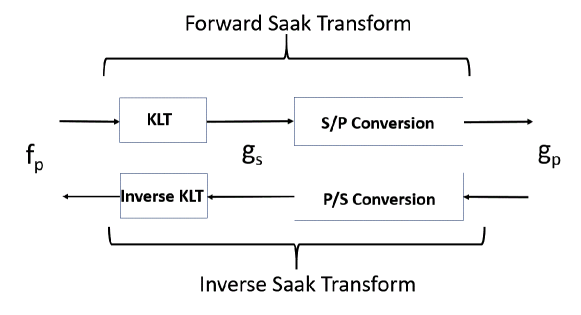
The block diagram of the forward and inverse Saak transforms is given in Fig. 1. The forward Saak transform consists of three steps: 1) building the optimal linear subspace approximation with orthonormal bases using the Karhunen-Lo$\acute{e}$ve transform (KLT) [16], 2) augmenting each transform kernel with its negative, 3) applying the rectified linear unit (ReLU) to the transform output. The second and third steps are equivalent to the sign-to-position (S/P) format conversion. The inverse Saak transform is conducted by performing the position-to-sign (P/S) format conversion before the inverse KLT. Generally speaking, the Saak transform is a process of converting the spatial variation to the spectral variation and the inverse Saak transform is a process of converting the spectral variation to the spatial variation.

As shown in Fig. 2, multi-stage Saak transforms are developed to transform images of a larger size. To begin with, we decompose an input into four quadrants recursively to form a quad-tree structure with its root being the full image and its leaf being a small patch of size $2\times 2$. Then, we conduct the Saak transform by merging four child nodes into one parent node stage by stage and from the leaf to the root. The whole process terminates when we reach the last stage (or the root of the tree) that has a spatial dimension of $1\times 1$. The signed KLT coefficients in each stage are called the Saak coefficients that can serve as discriminant features of the input image. Multi-stage Saak transforms provide a family of spatial-spectral representations. They are powerful representations to be used in many applications such as handwritten digits recognition, object classification, and image processing.

Fig. 2: Illustration of the forward and inverse multi-stage Saak transforms, where $\Phi^{p}$ is the set of the spatial-spectral representations in the $p$th stage, and $S_{p}$ and $S_{p}^{-1}$ are the forward and inverse Saak transforms between stages $(p-1)$ and $p$, respectively.

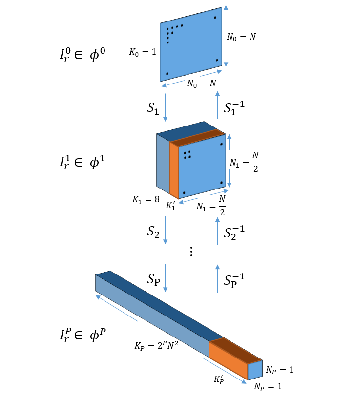
Only the lossless Saak transform was examined in [12]. For the lossless multi-stage Saak transforms, the spatial-spectral dimension in Stage $p$ is $2\times 2\times K_{p}$, where $K_{p}$ can be recursively computed as

$$K_{p}=2\times 4\times K_{(p-1)},\quad K_{0}=1,\quad p=1,2,\cdots.$$ (1)

The right-hand-side (RHS) consists of three terms. The first term is due to the S/P conversion. The second and third terms are from that the degree of freedom of the input cuboid and the output vector should be preserved through the KLT. As a consequence of Eq. (1), we have $K_{p}=8^{p}$. To avoid this exponential growth in terms of the stage number $p$, we can leverage the energy compaction property of the KLT and adopt the lossy Saak transform by replacing the KLT with the truncated KLT (or PCA).

Many useful properties are preserved in the lossy Saak transform such as the orthonormality of transform kernels and its capability to provide a family of spatial-spectral representations. However, there is a loss in reconstructing the original input. This is the reason that it is called the “lossy” transform. Since we deal with the classification problem, the exact reconstruction is of little concern here. To reduce the number of transform kernels, we select the leading $K^{{}^{\prime}}_{p}$ components that have the largest eigenvalues from all $K_{p}$ components in stage $p$. Empirically, we have $K^{{}^{\prime}}_{p}<<K_{p}$. This will be reported in Sec. 3.

Fig. 3: Illustration of the proposed Saak transform approach for pattern recognition. First, a subset of Saak coefficients is selected from each stage. Next, the feature dimension is further reduced. Finally, the reduced feature vector is sent to an SVM classifier.

Table 1: The classification accuracy (%) of the Saak transform approach for the MNIST dataset, where the first column indicates the kernel numbers used from stages 1-5 in the feature selection module while the second to the fifth columns indicate dimensions of the reduced feature dimension. The cutoff energy thresholds for the 2nd to 5th rows are 1%, 3%, 5% and 7% of the total energy, respectively.

#Kernels for each stage	32	64	128	256
All kernels	98.19	98.58	98.53	98.14
(4, 11, 16, 20, 17)	98.24	98.54	98.33	97.84
(4, 5, 8, 7, 9)	98.30	98.54	98.26	97.68
(4, 5, 5, 6, 7)	98.28	98.52	98.21	97.70
(4, 4, 4, 5, 5)	98.22	98.42	98.08	97.58

Table 2: The cosine similarity of transform kernels obtained with subsets and the whole set of MNIST training data, where the first column indicates the number of images using for training and the second to sixth columns indicate the cosine similarity in each stage.

Size	Stage 1	Stage 2	Stage 3	Stage 4	Stage 5
50000	0.9999	0.9999	0.9999	0.9999	0.9996
40000	0.9999	0.9999	0.9999	0.9999	0.9993
30000	0.9999	0.9999	0.9999	0.9999	0.9988
20000	0.9999	0.9999	0.9999	0.9996	0.9972
10000	0.9999	0.9999	0.9997	0.9992	0.9945

Table 3: The effect of the training set sizes on the MNIST dataset classification accuracy where the first row indicates the number of images used in transform kernel training and the second row indicates the classification accuracy (%).

Size	60000	5000	40000	30000	20000	10000
Accuracy	98.54	98.53	98.53	98.53	98.52	98.52

Table 4: The cosine similarity of transform kernels using fewer class numbers and the whole ten classes, where the first column indicates the object class number in training, and the second to sixth columns indicate the cosine similarity in each stage.

Class No.	Stage 1	Stage 2	Stage 3	Stage 4	Stage 5
8	0.9998	0.9996	0.9942	0.9940	0.9550
6	0.9982	0.9983	0.9866	0.9639	0.5586
4	0.9993	0.9990	0.9816	0.9219	0.4557
2	0.9390	0.9672	0.6567	0.6694	0.3294

3 Comparative Study

Table 5: The classification accuracy (%) on noisy images. All methods are trained on clean images. The first to fourth columns report the results of adding Salt and pepper noise as increasing noise level. The fifth to eighth columns display the results of adding Speckle noise, adding Gaussian noise, replacing background with uniform noise, and replacing background with texture images, respectively.

Method	S&P 1	S&P 2	S&P 3	S&P 4	Speckle	Gaussian	random_bg	texture_bg
LeNet-5	89.13	86.12	74.62	67.68	84.10	81.75	94.11	85.59
AlexNet	82.83	84.22	62.49	53.99	75.94	97,63	98.36	98.12
Saak	95.71	95.31	91.16	87.49	83.06	94.08	94.67	87.78

Fig. 4: The classification results of using fewer classes in training. where the blue line indicates the Saak transform approach and the green line indicates the LeNet-5 method.

We conduct a comparative study on the efficiency of lossless and lossy Saak transforms under a comparable accuracy level in Sec. 3.1 as well as the performance of the LeNet-5 and the Saak-transform-based solutions in terms of scalability and robustness in Secs. 3.2 and 3.3, respectively.

3.1 Efficiency

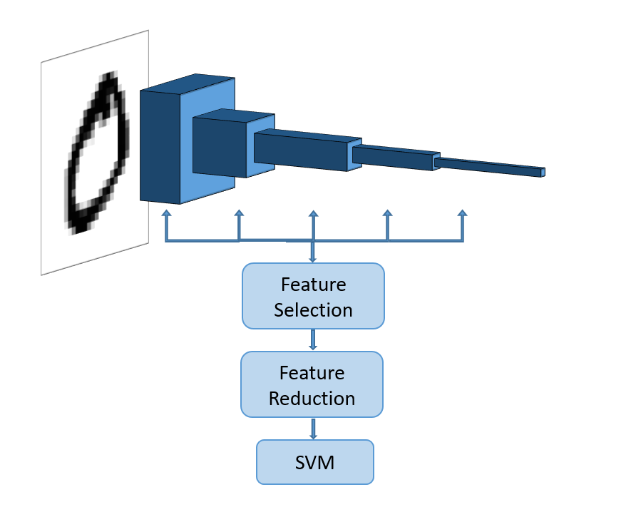
The proposed Saak-transform-based pattern recognition approach is illustrated in Fig. 3. For an input image of size $32\times 32$, we conduct five-stage lossy Saak transforms to compute spatial-spectral representations with spatial resolutions of $16\times 16(=256)$, $8\times 8(=64)$, $4\times 4(=16)$, $2\times 2(=4)$ and $1\times 1(=1)$. The feature selection module in the figure consists of two steps. For the first step, we select transform kernels using the largest eigenvalue criterion. This controls the number of Saak coefficients in each stage effectively while preserving the discriminative power. To give an example, if we choose transform kernels with their energy just greater than 3% of the total energy of the PCA, the kernel numbers from Stages 1 to 5 are 4, 5, 8, 7 and 9, respectively. Then, the number of the Saak features can be computed as

$$4\times 256+5\times 64+8\times 16+7\times 4+9\times 1=1,509,$$

For the second step, we adopt the F-test statistic (or score) in the ANalysis Of VAriance (ANOVA) [17] to select features that have the higher discriminant capability. That is, we order the features selected in the first step based on their F-test scores from the largest to the smallest, and select the top 75%. This will lead to a feature vector of dimension $1,509\times 0.75=1,132$. The feature selection module is followed by the feature reduction module, which is achieved by the PCA. We consider four reduced dimension cases of size $32$, $64$, $128$ and $256$, respectively, as shown in Table 1. Finally, we feed these reduced-dimension feature vectors to the SVM classifier in the SVM classification module. We compare different cutoff energy thresholds in selecting the number of transform kernels in each stage in Table 1. The first row gives the lossless Saak transform results and the best one is 98.58%. We see little performance degradation by employing the lossy Saak transform, yet its complexity is significantly reduced.

Fig. 5: Example of noisy test samples, where the first to fourth rows are noisy images with added Salt and pepper noise with an increasing noise level while the fifth to the eighth row are noisy images with added Speckle noise, Gaussian noise, background replaced by uniform noise, and background replaced by texture images, respectively.

3.2 Scalability

Here, we adopt multi-stage lossy Saak transforms with the energy threshold of 3% and reduce the feature dimension to 64 before applying the SVM classifier. We compare the average cosine similarity of the Saak transform kernels using the whole training set and the training subset in each stage in Table 2. We see from the table that the transform kernels are very stable, and the cosine similarity decreases slightly as going to higher stages. Even the lossy Saak transform is trained using only 10,000 samples, the cosine similarities between the resulting ones and the one trained using the whole training set consisting of 60,000 samples are still higher than 0.99. This shows that the trained kernels are very stable against the training data size. Next, we report the classification accuracy on the MNIST dataset in Table 3 and compare results among training sets of different sizes. It is interesting to see that we can obtain almost the same classification accuracy using lossy Saak coefficients based on a training dataset of a much smaller size.

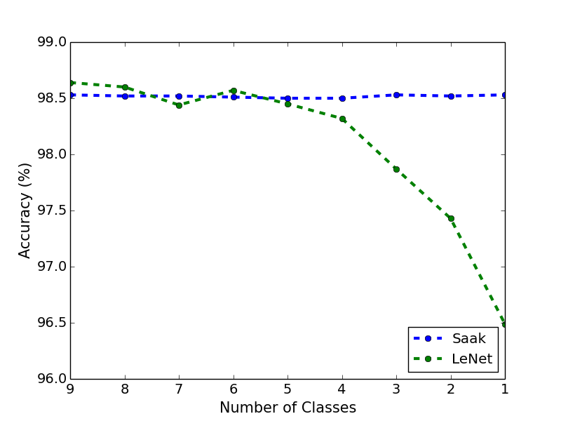
The experimental results of scalability against a varying object class number are shown in Table 4 and Fig. 4, where the class is arranged in increasing order. For example, if there are 4 classes in the training, they are digits 0, 1, 2, 3. We derive transform kernels with a subset of 10 digit classes and show the averaged cosine similarities in Table 4. As shown in the table, the transform kernels are relatively stable in the early stages. For example, the averaged cosine similarities of the first and the second stages are all above 0.9 even we only have one object class for training. The cosine similarities for later stages drop since the Saak coefficients of later stages capture the global view and they are effected more by decreasing the training classes. We see from Fig. 4 that the lossy Saak coefficients learned from fewer object classes can still handle the classification task of ten digits. In contrast, we train the convolutional layers of the LeNet-5 under the same above-mentioned condition while it fully connected (FC) layers are kept the same with ten output classes. Then, the performance of the LeNet-5 drops quickly when the object class number decreases. The Saak transform approach is more stable and it recognition accuracy is about the same even the number of training classes decreases. In general, the performance of the Saak transform offers a scalable solution to the handwritten digits recognition problem because the class features are obtained from sample class images. The LeNet-5 is more sensitive since it is built upon the end-to-end optimization framework. The network has to be re-trained whenever the object class number changes.

3.3 Robustness

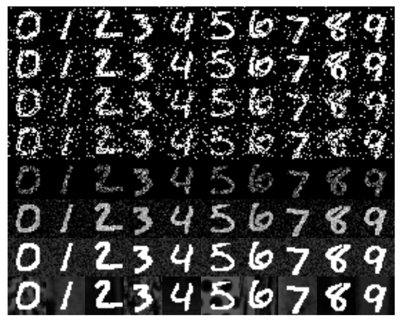
We may encounter undesirable noisy or low quality images in real-world applications, and need a robust method to handle these situations. To simulate the condition, we modify the MNIST dataset using two ways – adding noise and changing the background of the images as shown in Fig. 5. To test the robustness of classification methods fairly, we use only clean images in the training and the unseen noisy images in the testing. Table 5 compares the Saak transform based method, the LeNet-5 and the AlexNet. The LeNet-5 contains 2 CONV layers and 3 FC layers with around 60K parameters. The AlexNet consists of 5 CONV layers and 3 FC layers with around 60N parameters. For the Saak transform-based method, we set the energy threshold to 3% as described earlier and train the SVM classifier using 32D feature vectors. The results in Table 5 indicate that the performance of the lossy Saak transform method is less affected by noise, especially the Salt and Pepper noise. Although the Salt and Pepper noise is significantly increased in the column of S&P 4, our method can still achieve 87.49% accuracy. The AlexNet method is more robust to background change.

4 Conclusion and Future Work

A lossy Saak transform based approach was proposed to solve the handwritten digits recognition problem. This new approach has several advantages such as higher efficiency than the lossless Saak transform, scalability against the variation of training data size and object class numbers and robustness against noisy images. In the near future, we would like to apply the Saak transform approach to the general object classification problem with more challenging datasets such as CIFAR-10, CIFAR-100 and ImageNet.

References

- [1] Alex Krizhevsky, Ilya Sutskever, and Geoffrey E Hinton, “Imagenet classification with deep convolutional neural networks,” in Advances in neural information processing systems, 2012, pp. 1097–1105.
- [2] Yann LeCun et al., “Lenet-5, convolutional neural networks,” URL: http://yann. lecun. com/exdb/lenet, 2015.
- [3] Yann LeCun, Yoshua Bengio, and Geoffrey E. Hinton, “Deep learning,” Nature, vol. 521, pp. 436–444, 2015.
- [4] Li Wan, Matthew Zeiler, Sixin Zhang, Yann L Cun, and Rob Fergus, “Regularization of neural networks using dropconnect,” in Proceedings of the 30th international conference on machine learning (ICML-13), 2013, pp. 1058–1066.
- [5] Kaiming He and Jian Sun, “Convolutional neural networks at constrained time cost,” in Proceedings of the IEEE Conference on Computer Vision and Pattern Recognition, 2015, pp. 5353–5360.
- [6] Xiangyu Zhang, Jianhua Zou, Kaiming He, and Jian Sun, “Accelerating very deep convolutional networks for classification and detection,” IEEE transactions on pattern analysis and machine intelligence, vol. 38, no. 10, pp. 1943–1955, 2016.
- [7] Michael McCloskey and Neal J Cohen, “Catastrophic interference in connectionist networks: The sequential learning problem,” Psychology of learning and motivation, vol. 24, pp. 109–165, 1989.
- [8] Ian J Goodfellow, Mehdi Mirza, Da Xiao, Aaron Courville, and Yoshua Bengio, “An empirical investigation of catastrophic forgetting in gradient-based neural networks,” arXiv preprint arXiv:1312.6211, 2013.
- [9] Alhussein Fawzi, Seyed Mohsen Moosavi Dezfooli, and Pascal Frossard, “A geometric perspective on the robustness of deep networks,” Tech. Rep., Institute of Electrical and Electronics Engineers, 2017.
- [10] Seyed-Mohsen Moosavi-Dezfooli, Alhussein Fawzi, and Pascal Frossard, “Deepfool: a simple and accurate method to fool deep neural networks,” in Proceedings of the IEEE Conference on Computer Vision and Pattern Recognition, 2016, pp. 2574–2582.
- [11] Anh Nguyen, Jason Yosinski, and Jeff Clune, “Deep neural networks are easily fooled: High confidence predictions for unrecognizable images,” in Proceedings of the IEEE Conference on Computer Vision and Pattern Recognition, 2015, pp. 427–436.
- [12] C-C Jay Kuo and Yueru Chen, “On data-driven saak transform,” arXiv preprint arXiv:1710.04176, 2017.
- [13] Yann LeCun, Léon Bottou, Yoshua Bengio, and Patrick Haffner, “Gradient-based learning applied to document recognition,” Proceedings of the IEEE, vol. 86, no. 11, pp. 2278–2324, 1998.
- [14] C-C Jay Kuo, “Understanding convolutional neural networks with a mathematical model,” Journal of Visual Communication and Image Representation, vol. 41, pp. 406–413, 2016.
- [15] C-C Jay Kuo, “The cnn as a guided multilayer recos transform [lecture notes],” IEEE Signal Processing Magazine, vol. 34, no. 3, pp. 81–89, 2017.
- [16] Henry Stark and John W Woods, “Probability, random processes, and estimation theory for engineers,” Englewood Cliffs: Prentice Hall, 1986, 1986.
- [17] George EP Box, “Non-normality and tests on variances,” Biometrika, vol. 40, no. 3/4, pp. 318–335, 1953.