Narrowband Channel Estimation for Hybrid Beamforming Millimeter Wave Communication Systems with One-bit Quantization

Abstract

Millimeter wave (mmWave) spectrum has drawn attention due to its tremendous available bandwidth. The high propagation losses in the mmWave bands necessitate beamforming with a large number of antennas. Traditionally each antenna is paired with a high-speed analog-to-digital converter (ADC), which results in high power consumption. A hybrid beamforming architecture and one-bit resolution ADCs have been proposed to reduce power consumption. However, analog beamforming and one-bit quantization make channel estimation more challenging. In this paper, we propose a narrowband channel estimation algorithm for mmWave communication systems with one-bit ADCs and hybrid beamforming based on generalized approximate message passing (GAMP). We show through simulation that 1) GAMP variants with one-bit ADCs have better performance than do least-squares estimation methods without quantization, 2) the proposed one-bit GAMP algorithm achieves the lowest estimation error among the GAMP variants, and 3) exploiting more frames and RF chains enhances the channel estimation performance.

Index Terms—  millimeter wave, channel estimation, one-bit GAMP

1 Introduction

As cellular communication technologies consider adopting millimeter wave (mmWave) bands in need of tremendous available spectrum, communication systems need a large number of antennas to compensate the high propagation losses in such frequency bands. A corresponding number of radio frequency (RF) chains including high-speed analog-to-digital converters (ADCs) are to be paired with the antennas in a traditional sense, which inherently leads to high power consumption. A hybrid digital and analog beamforming architecture and low-resolution ADCs, therefore, were proposed in order to reduce power consumption primarily caused by those high-speed ADCs.

Low-resolution ADCs have recently been combined with hybrid beamforming. Hybrid beamforming with low-resolution ADCs yields comparable achievable rates to those systems with high-resolution ADCs in the low and medium SNR regimes [1]. The hybrid and full-digital beamforming architectures with low-resolution quantizers are shown to alternatively achieve better spectral and energy efficiency trade-off depending on characteristics of system components [2]. Spectral and energy efficiencies can be further enhanced by employing resolution adaptive ADCs with proper bit allocation algorithms [3, 4].

The combination of a hybrid beamforming architecture and low-resolution quantizers intended to reduce power consumption, however, makes channel estimation in such systems more challenging. Prior work regarding channel estimation in the context of mmWave can be grouped into a MIMO hybrid beamforming architecture with perfect quantizers [5, 6, 7, 8] or a MIMO fully-digital architecture with low-resolution quantizers [9, 10, 11]. Very few publications concern a system equipped with hybrid beamforming and low-resolution ADCs [12, 13]. In [12], The modified expectation-maximization algorithm is shown to yield acceptable channel estimation errors with low-resolution ADCs. In [13], generalized approximate message passing (GAMP) is proposed to use for wideband channel estimation, and four-bit ADCs are shown to achieve close performance to infinite bit ADCs at medium SNR. The channel estimation algorithms in [12, 13], however, are not specially designed for one-bit ADCs. Brief comparison of the mentioned prior work is given in Table 1.

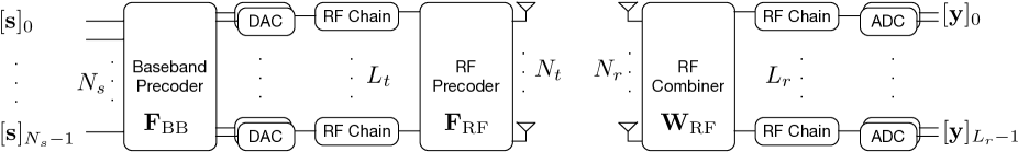
Fig. 1: A block diagram of a MIMO hybrid beamforming communication system. A transmitter and a receiver in this system are equipped with $N_{t}$ and $N_{r}$ antennas, and $L_{t}$ and $L_{r}$ RF chains, respectively.

In this paper, we propose a compressed sensing based channel estimation algorithm for a mmWave communication system equipped with one-bit ADCs and hybrid beamforming. GAMP and its variants have widely been used for channel estimation [13, 9, 10, 14]. One variant of GAMP used in this paper is named one-bit GAMP and is specifically developed for measurements taken with one-bit quantizers [15]. To make the algorithm better match a communication system model, we modify the algorithm to take the noise into account. Simulation results show that GAMP variants considered in this paper – GAMP [16], Expectation-Maximization Gaussian Mixture AMP (EM-GM-AMP) [17], and one-bit GAMP [15] – using one-bit ADCs perform better than does least-squares (LS) estimation without quantization. Among the variants, the modified one-bit GAMP achieves the lowest channel estimation error. The results also show that estimation performance can be enhanced by exploiting more frames and RF chains.

Table 1: Comparison of prior work

Ref.	Beamforming	ADC Resolution	Bandwidth
[5]	Hybrid	Infinite	Narrowband
[6]	Hybrid	Infinite	Narrowband
[7]	Hybrid	Infinite	Wideband
[8]	Hybrid	Infinite	Narrowband
[9]	Digital	Low (1–9 bits)	Wideband
[10]	Digital	Low (1 bit)	Narrowband
[11]	Digital	Low (1 bit)	Narrowband
[12]	Hybrid	Low (1–5 bits)	Narrowband
[13]	Hybrid	Low (1–4 bits)	Wideband

2 System Model

Consider a single-user MIMO hybrid beamforming mmWave system with $N_{t}$ transmit and $N_{r}$ receive antennas in the form of uniform linear arrays. The transmitter and receiver are equipped with $L_{t}$ ($\leq N_{t}$) and $L_{r}$ ($\leq N_{r}$) RF chains, respectively. The receiver employs quantizers that generate one-bit outputs. $N_{s}$ data streams are transmitted over narrowband MIMO channels where $N_{s}\leq\min(L_{t},L_{r})$. The transceivers are assumed to have the same number of RF chains, i.e. $L_{t}=L_{r}$. The block diagram for the system is illustrated in Fig. 1. The baseband signal vector transmitted at $N_{t}$ antennas in the $m^{\text{th}}$ frame can be expressed as $\mathbf{x}_{m}=\mathbf{F}_{\text{RF},m}\mathbf{F}_{\text{BB},m}\mathbf{s}_{m}$ where $\mathbf{F}_{\text{RF},m}\in\mathbb{C}^{N_{t}\times L_{t}}$ is the RF precoder, $\mathbf{F}_{\text{BB},m}\in\mathbb{C}^{L_{t}\times N_{s}}$ is the baseband precoder, and $\mathbf{s}_{m}\in\mathbb{C}^{N_{s}\times 1}$ is the training symbol vector with the constraint $\mathbb{E}[\mathbf{s}_{m}\mathbf{s}_{m}^{*}]=\frac{1}{N_{s}}\mathbf{I}_{N_{s}}$. The RF precoder is assumed to be built using a network of analog phase shifters; therefore, all elements of $\mathbf{F}_{\text{RF},m}$ should have the identical norm of $\frac{1}{N_{t}}$. In order to control the transmit power, the baseband precoder has a constraint such that $\lVert\mathbf{F}_{\text{RF},m}\mathbf{F}_{\text{BB},m}\rVert_{F}^{2}=N_{s}$. The quantized received baseband signal in the $m^{\text{th}}$ frame can be expressed as

$$\mathbf{y}_{m} =Q\left(\sqrt{\rho}\mathbf{W}_{\text{RF},m}^{\mathsf{H}}\mathbf{H}\mathbf{x}_{m}+\mathbf{W}_{\text{RF},m}^{\mathsf{H}}\mathbf{n}_{m}\right),$$ (1)

where $(\cdot)^{\mathsf{H}}$ denotes the conjugate transpose, $\rho$ denotes the average received power, $\mathbf{W}_{\text{RF},m}\in\mathbb{C}^{N_{r}\times L_{r}}$ is the RF combiner, $\mathbf{H}\in\mathbb{C}^{N_{r}\times N_{t}}$ is the flat-fading MIMO channel, and $\mathbf{n}_{m}\in\mathbb{C}^{N_{r}\times 1}\sim\mathcal{CN}(0,\sigma_{n}^{2}\mathbf{I})$ is the noise vector. As with the RF precoder, the RF combiner has a constraint that all elements have the identical norm of $\frac{1}{N_{r}}$. Since quantization of the received signal in this system is performed with one-bit ADCs, the quantization operator $Q(\cdot)$ extracts signs of real and imaginary components of a complex argument.

Using a geometric channel model, the normalized channel matrix $\mathbf{H}$ can be constructed by summing up $N_{p}$ paths. The azimuth angles of departure and arrival (AoD and AoA) associated with the $l^{\text{th}}$ path are denoted as $\theta_{tl}$ and $\theta_{rl}$, respectively. Both $\theta_{tl}$ and $\theta_{rl}$ are uniform random variables distributed over $[0,2\pi)$. Therefore, $\mathbf{H}$ can be expressed as

$$\ \mathbf{H}=\sqrt{\frac{N_{r}N_{t}}{N_{p}}}\sum_{l=0}^{N_{p}-1}\alpha_{l}\mathbf{a}_{\text{r}}(\theta_{rl})\mathbf{a}_{\text{t}}^{\mathsf{H}}(\theta_{tl}),$$

where $\alpha_{l}\sim\mathcal{CN}(0,\sigma_{\alpha}^{2})$ is the complex channel gain of the $l^{\text{th}}$ path, $\mathbf{a}_{\text{t}}(\cdot)\in\mathbb{C}^{N_{t}\times 1}$ and $\mathbf{a}_{\text{r}}(\cdot)\in\mathbb{C}^{N_{r}\times 1}$ are the transmit and receive array response vectors at the given AoD and AoA, respectively. The channel matrix $\mathbf{H}$ is constrained to have $\mathbb{E}[\left\lVert\mathbf{H}\right\lVert_{F}^{2}]=N_{t}N_{r}$ to maintain a constant channel power on average. $\mathbf{H}$ can also be represented with the virtual channel representation as

$$\mathbf{H}=\mathbf{U}_{\text{r}}\mathbf{H}_{\text{v}}\mathbf{U}_{\text{t}}^{\mathsf{H}},$$

where $\mathbf{U}_{\text{t}}$ and $\mathbf{U}_{\text{r}}$ denote the normalized $N_{t}$-point and $N_{r}$-point unitary Discrete Fourier Transform (DFT) matrices, and $\mathbf{H}_{\text{v}}\in\mathbb{C}^{N_{r}\times N_{t}}$ is the virtual channel matrix in the angular domain. As AoDs and AoAs are random in each channel realization, the array response vectors do not always align with columns of DFT matrices. This misalignment causes spectral leakage which degrades the performance of channel estimation algorithms. The leakage effect can be seen by comparing two subfigures in Fig. 2. When AoDs and AoAs are perfectly aligned, or equivalently, antenna array response vectors can be expressed with the DFT matrix columns, $\mathbf{H}_{\text{v}}$ has exactly $N_{p}$ non-zero elements as seen in Fig. 2(a). Otherwise, each beam leaks into adjacent bins, which results in spreads around them as shown in Fig. 2(b). In Section 4, performance degradation due to the leakage effect is discussed.

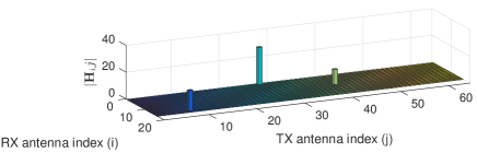
(a)

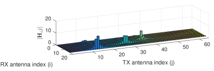
(b)

Fig. 2: Magnitude of virtual channel matrix with $N_{p}=3$ in the angular domain. Spreads shown in (b) illustrate leakage into adjacent bins.

3 Compressed Sensing Channel Estimation

For estimation of the sparse virtual channel, the $m^{\text{th}}$ received frame in (1) is reformulated into a vector form using $\text{vec}(\mathbf{A}\mathbf{B}\mathbf{C})=(\mathbf{C}^{\mathsf{T}}\otimes\mathbf{A})\text{vec}(\mathbf{B})$. Then $\mathbf{y}_{m}$ is rewritten as

$$\mathbf{y}_{m} =Q\Big{(}\sqrt{\rho}\left(\mathbf{s}_{m}^{\mathsf{T}}\mathbf{F}_{\text{BB},m}^{\mathsf{T}}\mathbf{F}_{\text{RF},m}^{\mathsf{T}}\otimes\mathbf{W}_{\text{RF},m}^{\mathsf{H}}\right)\left(\mathbf{U}_{\text{t}}^{*}\otimes\mathbf{U}_{\text{r}}\right)$$

$$\times\text{vec}(\mathbf{H}_{\text{v}})+\tilde{\mathbf{n}}_{m}\Big{)},$$

where $(\cdot)^{*}$ denotes the complex conjugation, $\otimes$ denotes the Kronecker product operator, and $\tilde{\mathbf{n}}_{m}$ denotes $\mathbf{W}_{\text{RF},m}^{\mathsf{H}}\mathbf{n}_{m}$. For simple notation, we define $\mathbf{\Phi}=[\mathbf{\Gamma}_{0}^{\mathsf{T}},\mathbf{\Gamma}_{1}^{\mathsf{T}},\cdots,\mathbf{\Gamma}_{M-1}^{\mathsf{T}}]^{\mathsf{T}}$, $\mathbf{\Psi}=\mathbf{U}_{\text{t}}^{*}\otimes\mathbf{U}_{\text{r}}$, and $\tilde{\mathbf{n}}=[\tilde{\mathbf{n}}_{0}^{\mathsf{T}},\tilde{\mathbf{n}}_{1}^{\mathsf{T}},\cdots,\tilde{\mathbf{n}}_{M-1}^{\mathsf{T}}]^{\mathsf{T}}$ where $\mathbf{\Gamma}_{m}=\mathbf{s}_{m}^{\mathsf{T}}\mathbf{F}_{\text{BB},m}^{\mathsf{T}}\mathbf{F}_{\text{RF},m}^{\mathsf{T}}\otimes\mathbf{W}_{\text{RF},m}^{\mathsf{H}}$. By stacking $M$ received frame vectors, $\mathbf{y}$ is obtained as

$$\mathbf{y} =\left[\mathbf{y}_{0}^{\mathsf{T}},\mathbf{y}_{1}^{\mathsf{T}},\cdots,\mathbf{y}_{M-1}^{\mathsf{T}}\right]^{\mathsf{T}}=Q\left(\sqrt{\rho}\mathbf{\Phi}\mathbf{\Psi}\mathbf{\widetilde{h}}_{\text{v}}+\tilde{\mathbf{n}}\right),$$

where $\mathbf{\widetilde{h}}_{\text{v}}$ denotes $\text{vec}(\mathbf{H}_{\text{v}})$. We define the unquantized received vector $\mathbf{\widetilde{r}}=\mathbf{\widetilde{W}}\mathbf{\widetilde{h}}_{\text{v}}+\tilde{\mathbf{n}}$ where $\mathbf{\widetilde{W}}=\sqrt{\rho}\mathbf{\Phi}\mathbf{\Psi}$. To separate in-phase and quadrature components, it is further reformulated as $\mathbf{r}=\mathbf{W}\mathbf{h}_{\text{v}}+\mathbf{n}$ where

$$\mathbf{r} =\begin{bmatrix}\Re{\{\mathbf{\widetilde{r}}\}}\\ \Im{\{\mathbf{\widetilde{r}}\}}\end{bmatrix},\mathbf{W}=\begin{bmatrix}\Re{\{\mathbf{\widetilde{W}}\}}&-\Im{\{\mathbf{\widetilde{W}}\}}\\ \Im{\{\mathbf{\widetilde{W}}\}}&\Re{\{\mathbf{\widetilde{W}}\}}\end{bmatrix},$$

$$\mathbf{h}_{\text{v}} =\begin{bmatrix}\Re{\{\mathbf{\widetilde{h}}_{\text{v}}\}}\\ \Im{\{\mathbf{\widetilde{h}}_{\text{v}}\}}\end{bmatrix},\text{and }\mathbf{n}=\begin{bmatrix}\Re{\{\tilde{\mathbf{n}}\}}\\ \Im{\{\tilde{\mathbf{n}}\}}\end{bmatrix}.$$

Algorithm 1 One-bit GAMP

1:Initialize:

2:      $t=0$, $\hat{\mathbf{h}}_{\text{v}}^{t}=\mathbb{E}[\mathbf{h}_{\text{v}}]$, $\mathbf{v}^{t}_{\mathbf{h}_{\text{v}}}=\text{Var}[{\mathbf{h}_{\text{v}}}]$, $\hat{\mathbf{s}}^{t}=0$,

3:for $t=1,\cdots,T$ do

4:Measurement update:

5:     $\mathbf{v}^{t+1}_{p}=(\mathbf{W}\bullet\mathbf{W})\mathbf{v}_{\mathbf{h}_{\text{v}}}^{t}$,

6:     $\hat{\mathbf{p}}^{t+1}=\mathbf{W}\mathbf{h}_{\text{v}}^{t}-\mathbf{v}_{p}^{t+1}\bullet\hat{\mathbf{s}}^{t}$,

7:     for all $i$ do

8:         $\left[\hat{\mathbf{s}}^{t+1}\right]_{i}=\frac{1}{[\mathbf{v}_{p}^{t+1}]_{i}+\sigma^{2}_{\tilde{n}}}(\mathbb{E}\left[r|r\in Q^{-1}([\mathbf{y}]_{i})\right]-$

9:      $[\hat{\mathbf{p}}^{t+1}]_{i})$,

10:         $\left[\mathbf{v}_{s}^{t+1}\right]_{i}=\frac{1}{[\mathbf{v}_{p}^{t+1}]_{i}+\sigma^{2}_{\tilde{n}}}\left(1-\frac{\text{Var}\left[r|r\in Q^{-1}([\mathbf{y}]_{i})\right]}{[\mathbf{v}_{p}^{t+1}]_{i}+\sigma^{2}_{\tilde{n}}}\right)$,

11:     end for

12:Estimation update:

13:     $\mathbf{v}_{r}^{t+1}=\left((\mathbf{W}\bullet\mathbf{W})^{\mathsf{T}}\mathbf{v}_{s}^{t+1}\right)^{-1}$,

14:     $\hat{\mathbf{r}}^{t+1}=\hat{\mathbf{h}}_{\text{v}}^{t}+\mathbf{v}_{r}^{t+1}\bullet\left(\mathbf{W}^{\mathsf{T}}\hat{\mathbf{s}}^{t+1}\right)$,

15:     for all $i$ do

16:         $\left[\hat{\mathbf{h}}_{\text{v}}^{t+1}\right]_{i}=\mathbb{E}\left[h_{\text{v}}|[\hat{\mathbf{r}}^{t+1}]_{i}\right]$,

17:         $\left[\mathbf{v}_{\mathbf{h}_{\text{v}}}^{t+1}\right]_{i}=\text{Var}\left[h_{\text{v}}|[\hat{\mathbf{r}}^{t+1}]_{i}\right]$,

18:     end for

19:end for

For sparse reconstruction of the virtual channel vector, we consider one-bit GAMP which is specifically developed for measurements taken with one-bit quantizers [15]. We modify the proposed algorithm to take into consideration the additive noise and set the quantization threshold to zero. The modified algorithm is described in Algorithm 1 where $\bullet$ denotes the element-wise product and $[\cdot]_{i}$ denotes the $i^{\text{th}}$ element in a vector. The expected value and the variance in lines 6 and 7 are with respect to $r\sim\mathcal{N}([\hat{\mathbf{p}}]_{i},[\mathbf{v}_{p}^{t+1}]_{i}+\sigma^{2}_{n})$. Those in lines 12 and 13 are with respect to $p_{h_{\text{v}}|[\hat{\mathbf{r}}^{t+1}]_{i}}(h_{\text{v}}|[\hat{\mathbf{r}}^{t+1}]_{i})$ which is proportional to the product of $p_{h_{\text{v}}}(h_{\text{v}})$ and the Gaussian PDF with mean $[\hat{\mathbf{r}}^{t+1}]_{i}$ and variance $[\mathbf{v}_{r}^{t+1}]_{i}$.

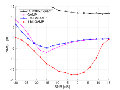
(a)

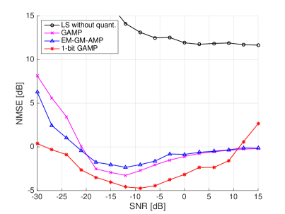
(b)

Fig. 3: NMSE of four channel estimation algorithms: LS, GAMP, EM-GM-AMP and one-bit GAMP (proposed). The leakage effect is considered in (b) and degrades channel estimation performance.

4 Numerical Results

In this section, we evaluate channel estimation performance of the modified one-bit GAMP and compare it with other algorithms that include LS estimation, GAMP, and EM-GM-AMP [18]. The normalized mean squared error (NMSE) is used as a performance metric:

$$\text{NMSE}=\mathbb{E}\left[{\lVert\mathbf{H}-\hat{\mathbf{H}}\rVert_{F}^{2}}/{\left\lVert\mathbf{H}\right\lVert_{F}^{2}}\right].$$

For simulation, system parameters used in this section are as follows unless otherwise stated: $N_{t}=64$, $N_{r}=16$, $L_{t}=4$, $L_{r}=4$, $N_{p}=2$, and $M=64$. Columns of a Hadamard matrix are used for training symbol vectors.

Fig. 3 shows NMSE of four channel estimation algorithms. For comparison purposes, the LS estimator is without signal quantization while others use one-bit ADCs. Simulated channels for Fig. 3(a) are intentionally constructed to avoid the leakage effect whereas those for Fig. 3(b) do not have such constraint. As seen in both subfigures, the LS estimator without quantization achieves far worse performance than do GAMP variants with one-bit ADCs. One-bit GAMP yields the lowest estimation errors among the considered algorithms in both subfigures. Comparing two subfigures, we can see that all algorithms suffer performance degradation due to the leakage effect. Figures henceforth are with one-bit GAMP and channels that experience the leakage effect.

The number of RF chains affects the channel estimation performance as shown in Fig. 4. Two, four and eight pairs of RF chains are plotted. More RF chains improve the performance across the considered SNR range. From a compressed sensing perspective, this is because more RF chains allow longer measurement vector.

Fig. 5 shows effects of the number of frames on channel estimation performance in various SNR regimes. As shown in Fig. 3(b), the minimum NMSE can be obtained around an SNR of -9 dB, which corresponds to the fact that the curve for -9 dB SNR in Fig. 5 has lower NMSE than the others. Regardless of SNR values, estimation error decreases as more frames are used for estimation. It is expected since coherence of the measurement matrix declines with the increasing number of frames for any SNR.

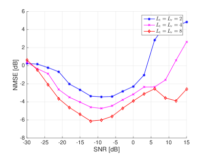
Fig. 4: NMSE as a function of RF chains. More RF chains improve channel estimation performance.

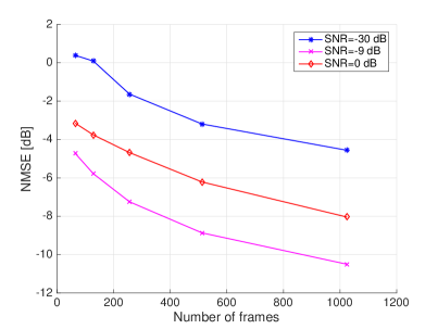
Fig. 5: NMSE as a function of frames. For any SNR, estimation error decreases with increasing number of frames.

5 Conclusion

In this paper, we proposed a channel estimation algorithm for a mmWave communication system with one-bit quantizers and hybrid beamforming based on GAMP. This one-bit GAMP method is specifically designed for measurements taken with one-bit ADCs, and we modified it to take into account the thermal noise. Simulation results showed that GAMP variants with one-bit ADCs achieve better performance than LS without quantization, and that the proposed algorithm yields the lowest channel estimation error among the GAMP variants. Results also showed that the channel estimation performance can be enhanced by exploiting more frames and RF chains.

References

- [1] J. Mo, A. Alkhateeb, S. Abu-Surra, and R. W. Heath, “Hybrid architectures with few-bit ADC receivers: Achievable rates and energy-rate tradeoffs,” IEEE Trans. Wireless Commun., vol. 16, no. 4, pp. 2274–2287, Apr. 2017.
- [2] W. B. Abbas, F. Gomez-Cuba, and M. Zorzi, “Millimeter wave receiver efficiency: A comprehensive comparison of beamforming schemes with low resolution ADCs,” IEEE Trans. Wireless Commun., to be published.
- [3] J. Choi, B. L. Evans, and A. Gatherer, “Resolution-adaptive hybrid MIMO architectures for millimeter wave communications,” IEEE Trans. Signal Process., vol. 65, no. 23, pp. 6201–6216, Dec. 2017.
- [4] J. Choi, B. L. Evans, and A. Gatherer, “ADC bit allocation under a power constraint for mmWave massive MIMO communication receivers,” in Proc. IEEE Int. Conf. Acoust., Speech, Sig. Process., Mar. 2017, pp. 3494–3498.
- [5] A. Alkhateeb, O. El Ayach, G. Leus, and R. W. Heath, “Channel estimation and hybrid precoding for millimeter wave cellular systems,” IEEE J. Sel. Topics in Sig. Process., vol. 8, no. 5, pp. 831–846, Oct. 2014.
- [6] S. Park and R. W. Heath, “Spatial channel covariance estimation for mmWave hybrid MIMO architecture,” in Proc. Asilomar Conf. Sig., Sys., and Comp., Nov. 2016, pp. 1424–1428.
- [7] K. Venugopal, A. Alkhateeb, R. W. Heath, and N. González-Prelcic, “Time-domain channel estimation for wideband millimeter wave systems with hybrid architecture,” in Proc. IEEE Int. Conf. Acoust., Speech, Sig. Process., Mar. 2017, pp. 6493–6497.
- [8] A. Alkhateeb, G. Leusz, and R. W. Heath, “Compressed sensing based multi-user millimeter wave systems: How many measurements are needed?,” in Proc. IEEE Int. Conf. Acoust., Speech, Sig. Process., Apr. 2015, pp. 2909–2913.
- [9] J. Mo, P. Schniter, and R. W. Heath, “Channel estimation in broadband millimeter wave MIMO systems with few-bit ADCs,” arXiv:1610.02735, 2016.
- [10] J. Mo, P. Schniter, N. González-Prelcic, and R. W. Heath, “Channel estimation in millimeter wave MIMO systems with one-bit quantization,” in Proc. Asilomar Conf. Sig., Sys., and Comp., Nov. 2014, pp. 957–961.
- [11] C. Rusu, R. Méndez-Rial, N. González-Prelcic, and R. W. Heath, “Adaptive one-bit compressive sensing with application to low-precision receivers at mmWave,” in Proc. IEEE Global Commun. Conf., Dec. 2015, pp. 1–6.
- [12] J. Rodríguez-Fernández, K. Venugopal, N. González-Prelcic, and R. W. Heath, “Channel estimation in mixed hybrid-low resolution MIMO architectures for mmWave communication,” in Proc. Asilomar Conf. Sig., Sys., and Comp., Nov. 2016, pp. 768–773.
- [13] J. Mo, P. Schniter, and R. W. Heath, “Channel estimation in broadband millimeter wave mimo systems with few-bit adcs,” IEEE Trans. Signal Process., vol. 66, no. 5, pp. 1141–1154, March 2018.
- [14] J. García, J. Munir, K. Roth, and J. A. Nossek, “Channel estimation and data equalization in frequency-selective MIMO systems with one-bit quantization,” arXiv:1609.04536, 2016.
- [15] U. S. Kamilov, A. Bourquard, A. Amini, and M. Unser, “One-bit measurements with adaptive thresholds,” IEEE Signal Process. Lett., vol. 19, no. 10, pp. 607–610, Oct. 2012.
- [16] S. Rangan, “Generalized approximate message passing for estimation with random linear mixing,” in Proc. IEEE Int. Symp. on Inform. Theory, July 2011, pp. 2168–2172.
- [17] J. P. Vila and P. Schniter, “Expectation-maximization gaussian-mixture approximate message passing,” IEEE Trans. Signal Process., vol. 61, no. 19, pp. 4658–4672, Oct. 2013.
- [18] J. Sung and B. L. Evans, “Channel estimation for hybrid beamforming millimeter wave communication systems with one-bit quantization,” Software Release, Oct. 27, 2017, http://users.ece.utexas.edu/~bevans/projects/mimo/software/channel/.