The fate of close encounters between binary stars and binary supermassive black holes
Abstract
The evolution of main sequence binaries that reside in the Galactic Centre can be heavily influenced by the central super massive black hole (SMBH). Due to these perturbative effects, the stellar binaries in dense environments are likely to experience mergers, collisions or ejections through secular and/or non-secular interactions. More direct interactions with the central SMBH are thought to produce hypervelocity stars (HVSs) and tidal disruption events (TDEs). In this paper, we use N-body simulations to study the dynamics of stellar binaries orbiting a central SMBH primary with an outer SMBH secondary orbiting this inner triple. The effects of the secondary SMBH on the event rates of HVSs, TDEs and stellar mergers are investigated, as a function of the SMBH-SMBH binary mass ratio. Our numerical experiments reveal that, relative to the isolated SMBH case, the TDE and HVS rates are enhanced for, respectively, the smallest and largest mass ratio SMBH-SMBH binaries. This suggests that the observed event rates of TDEs and HVSs have the potential to serve as a diagnostic of the mass ratio of a central SMBH-SMBH binary. The presence of a secondary SMBH also allows for the creation of hypervelocity binaries. Observations of these systems could thus constrain the presence of a secondary SMBH in the Galactic Centre.
keywords:
black hole physics-Galaxy:numerical-stellar dynamics1 Introduction
Supermassive black holes (SMBHs) ubiquitously reside at the centres of galaxies (e.g., Kormendy & Ho, 2013). Observations show that, in the inner 1 parsec (pc) of our own Milky Way, the gravitational potential is dominated by a central SMBH with mass 4 106 M⊙ (e.g., Alexander, 2005; Gillessen et al., 2017). In the immediate vicinity of the SMBH, there exists a a densely packed and complicated stellar environment. The relatively high stellar density at the center of the Milky Way and the small mass of the SMBH imply that the relaxation time of two-body interaction could be as short as a Gyr, but longer estimates have also been quoted (e.g. Merritt, 2013).
Much uncertainty persists in understanding the constituents of this inner Keplerian-dominated region. Some parameter space exists that permits for the presence of an IMBH with mass 103-104 M⊙ (Yu & Tremaine, 2003; Gualandris, Portegies Zwart & Sipior, 2005; Gualandris & Merritt, 2009). A handful of compact binary star systems have also been observed in the Galactic Centre (Martins et al., 2006). These bound state binaries orbiting the central SMBH form hierarchical triple systems, and are hence subject to both secular dynamical effects and chaotic perturbations from other objects (e.g. Antonini et al., 2010; Leigh et al., 2016a). This has the potential to stimulate a high rate of observable dynamical phenomena, such as hypervelocity stars and tidal disruption events.
Gravitational encounters involving stellar binaries and an SMBH operating on characteristic timescales shorter than the secular timescale have been studied extensively: (i) When the stellar binaries are on low angular momentum orbits, the stellar binaries are considered to be easily broken up due to the strong tidal field of the SMBH. As a result, one component is captured by the SMBH, while the other is ejected at high velocity. This is one mechanism believed to produce hypervelocity stars (HVSs) (e.g., Hills, 1988; Yu & Tremaine, 2003; Antonini et al., 2010); (ii) Conversely, the stars in a binary can be tidally disrupted by the SMBH if the relative distance is less than the tidal disruption radius of a given binary component. The subsequent accretion of the stellar debris by the SMBH results in a strong flare of electromagnetic radiation, called to a tidal disruption event (TDE) (e.g., Hills, 1975; Rees, 1988; Phinney, 1989; Gezari et al., 2012; Mandel & Levin, 2015); (iii) Finally, such a close interaction between the SMBH and the stellar binary may lead to a physical collision between the two components of the binary (e.g., Ginsburg & Loeb, 2007).
If the orbital plane of the stellar binary is inclined relative to the plane of its orbit about the SMBH by , the eccentricity and inclination of the binary orbit will experience periodic oscillations on a secular timescale, known as Lidov-Kozai (LK) oscillations (e.g., Lidov, 1962; Kozai, 1962). Here, the orbital eccentricity of the binary slowly increases while the inclination decreases, conserving angular momentum, and vice versa. The effects of LK oscillations include the formation of a number of exotic astrophysical systems (e.g., Eggleton & Kiseleva–Eggleton, 2001; Fabrycky & Tremaine, 2007; Holman, Touma,& Tremaine, 1997; Innanen et al., 1997; Wu & Murray, 2003; Storch, Anderson, & Lai, 2014; Liu, Lai, & Yuan, 2015; Anderson, Storch, & Lai, 2016). For example, the presence of a central massive BH can accelerate the rate of black hole binary mergers due LK oscillations, both at the centres of galaxies and globular clusters (e.g., Blaes et al., 2002; Miller & Hamilton, 2002; Wen, 2003; Antonini, Murray & Mikkola, 2014; Fragione, Ginsburg, & Kocsis, 2017). Similarly, LK oscillations can stimulate Type Ia supernova from white-dwarf binary mergers (e.g., Thompson, 2011; Prodan, Murray, & Thompson, 2013) or direct collisions between main-sequence stars and hence blue straggler formation (e.g., Katz & Dong, 2012; Kushnir et al., 2013; Leigh et al., 2016b). An enhanced rate of stellar TDEs might also be expected in the presence of a massive BH, due to the eccentric LK mechanism alone (e.g., Li et al., 2015; Liu, Wang, & Yuan, 2017).
In this paper, we consider stellar binaries orbiting around a central primary SMBH, perturbed by a distant secondary SMBH. We study the effects of different mass ratios of the SMBH-SMBH binary in determining the relative rates of HVS production, TDE production and binary mergers. The presence of a secondary SMBH orbiting the inner SMBH-binary star triple serves to perturb and/or accelerate the secular dynamical evolution of the inner triple system.
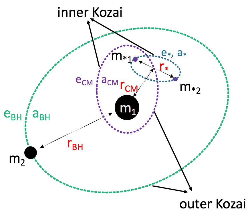
The SMBH-SMBH binary, together with the stellar binary, can be decomposed into two separate hierarchical triple systems. These are the SMBH-star-star triple and the SMBH-stellar binary-SMBH triple. As anticipated, the secular dynamical processes in the inner triple are accelerated by the presence of the secondary SMBH, leading to an enhancement in the overall rate of observable astronomical events (TDEs, HVSs, mergers). When the inner triple has a relative orbital inclination that lies in the range , LK oscillations occur. Subsequently, the eccentricity of the stellar binary can be excited, leading to a merger between the two binary components. Conversely, when LK oscillations in the outer triple are operating, the stellar binary orbit about the primary SMBH can be excited to very high eccentricities. If the periastron distance corresponding to this orbit reaches the tidal disruption radius, the binary will be disrupted, producing a TDE and/or an HVS. The mass of the secondary SMBH plays a fundamental role in this four-body system, by affecting the time scales for LK oscillations to operate.
Our paper is organized as follows. In Section 2, we introduce the geometry of the four-body system. Through a comparison of the relevant timescales, we characterize the parameter space where outer LK oscillations dominate over inner LK oscillations and vice versa. In Section 3, we describe the numerical setup and initial conditions for our N-body simulations. In Section 4, we present the results of our N-body simulations, and explore the evolution of stellar binaries orbiting inside the orbit of an SMBH-SMBH binary as a function of its mass ratio. Our conclusions are summarized in Section 5.
2 A stellar binary orbiting an SMBH binary
As shown in Figure 1, we label the masses of the stars by and (i.e., the stellar binary components), the mass of the primary SMBH by , and the mass of the secondary SMBH by . For the orbital parameters, we use to denote the semi-major axes, the eccentricities and the separations between the two components of each binary. Here, the subscripts “*, CM, BH” denote, the (internal) orbit of the stellar binary, the orbit of the stellar binary about the primary SMBH and the orbit of the secondary SMBH about the primary SMBH, respectively. Geometrically, the four-body system can be decomposed in to an inner triple (SMBH-star-star) and an outer triple (SMBH-stellar binary-SMBH). In each triple system, if the inclination between two orbital planes is and , then the eccentricity and inclination of the inner orbit will experience periodic oscillations on a secular timescale, known as Lidov-Kozai (LK) oscillations (e.g., Lidov 1962; Kozai 1962). If the outer BH is on a highly inclined orbit around the binary and at a moderate distance, the LK oscillations breakdown. Non-secular and chaotic effects will be introduced into the system, which have the potential to lead to a rapid merger in the inner orbit(Antonini, Murray, & Mikkola, 2014). In such a four-body system, the competition between LK resonances in the inner and outer triple configurations, together with non-secular and chaotic effects, could serve as an important catalyst for astronomically observable events such as the production of HVSs, TDEs and stellar mergers.
2.1 Basic relations
Several physical mechanisms play a fundamental role in our simulations. They are summarized in the following:
-
1.
Due to their low densities, main-sequence stars are easily tidally disrupted in the vicinity of an SMBH. Tidal disruption occurs for stars that approach the SMBH more closely than ,
(1) where is the mass of the SMBH, the mass of the star and the radius of the star. In our simulations, we use the mass-radius relation which yields for (e.g., Hansen, Kawaler, & Trimble, 2004).
-
2.
Stellar binaries will be broken apart by the SMBH if the stellar binary enters the tidal breakup radius ,
(2) where is the separation of the two components in the stellar binary.
-
3.
The stellar binary remains bound to the black hole within the Hill sphere of the primary SMBH (). The radius of the Hill sphere is
(3) For stellar binaries within the Hill sphere, there is no chance either of tidal disruption by the secondary SMBH () or of being ejected from the system by the slingshot effect induced by the secondary SMBH (). For large mass ratios of the SMBH binary, the stellar binaries could reside outside of the Hill sphere. For these stellar binaries, the hierarchical structure of the four-body system will be broken. The LK oscillations can no longer operate and affect the internal system evolution.
-
4.
The hierarchical condition for a stable triple system is
(4) For binaries whose orbital parameters satisfy this hierarchical condition, the LK effect can excite the binary orbit. This could ultimately lead to decoupling of the binary followed by tidal disruptions, mergers, or HVSs. At the quadrupole level, the LK effect defines the maximum value of the excited eccentricity to be , where is the initial inclination between the inner and outer orbital planes of the triple system. Combining this with Eq (1) and the stellar mass-radius relation, we can calculate analytically the rates of single TDEs and mergers.
For those binaries that do not satisfy the hierarchical condition, a chaotic effect is introduced into the system. Nevertheless, scattering experiments reveal that the binary orbit can still be excited in the strong interaction region where (e.g., Chen et al., 2009).
-
5.
The hardening radius of the black hole binary is
(5) where is the velocity dispersion of the stellar cusp surrounding the primary SMBH.
2.2 Time scales
In order to identify the parameter space where the Lidov-Kozai effect becomes dominant, we consider the different sources of apsidal precession in galactic nuclei hosting SMBHs. For the inner triple system, the stellar binary is immersed in a dense environment. Other perturbative effects may come into play and affect the evolution of the stellar binary, or even change the outcome of an otherwise secular interaction.
Binaries orbited by a highly inclined perturber will undergo LK oscillations. In the inner triple, the corresponding timescale at the approximation of the quadrupole level is (e.g., Lidov, 1962; Kozai, 1962)
| (6) |
where is the mean motion of the stellar binary.
Similarly, in the outer triple, the corresponding timescale at the quadrupole level is
| (7) |
where is the mean motion of the stellar binary orbiting the primary SMBH.
If the stellar binary orbital separation at pericentre is sufficiently small, additional effects such as general relativity (GR) can dominate the tidal torque exerted by the outer binary, suppressing the excitation of its eccentricity (e.g., Blaes et al., 2002; Naoz et al., 2013a; Naoz, 2016). The timescale for precession of the argument of periapsis caused by the first order post Newtonian (PN) correction in the inner and outer orbits is
| (8) |
and
| (9) |
respectively. The interaction between the inner and outer binaries at 1 PN order adds an additional term in the equation of motion. The related timescale is given by (e.g., Naoz et al., 2013a; Will, 2014a, b)
| (10) |
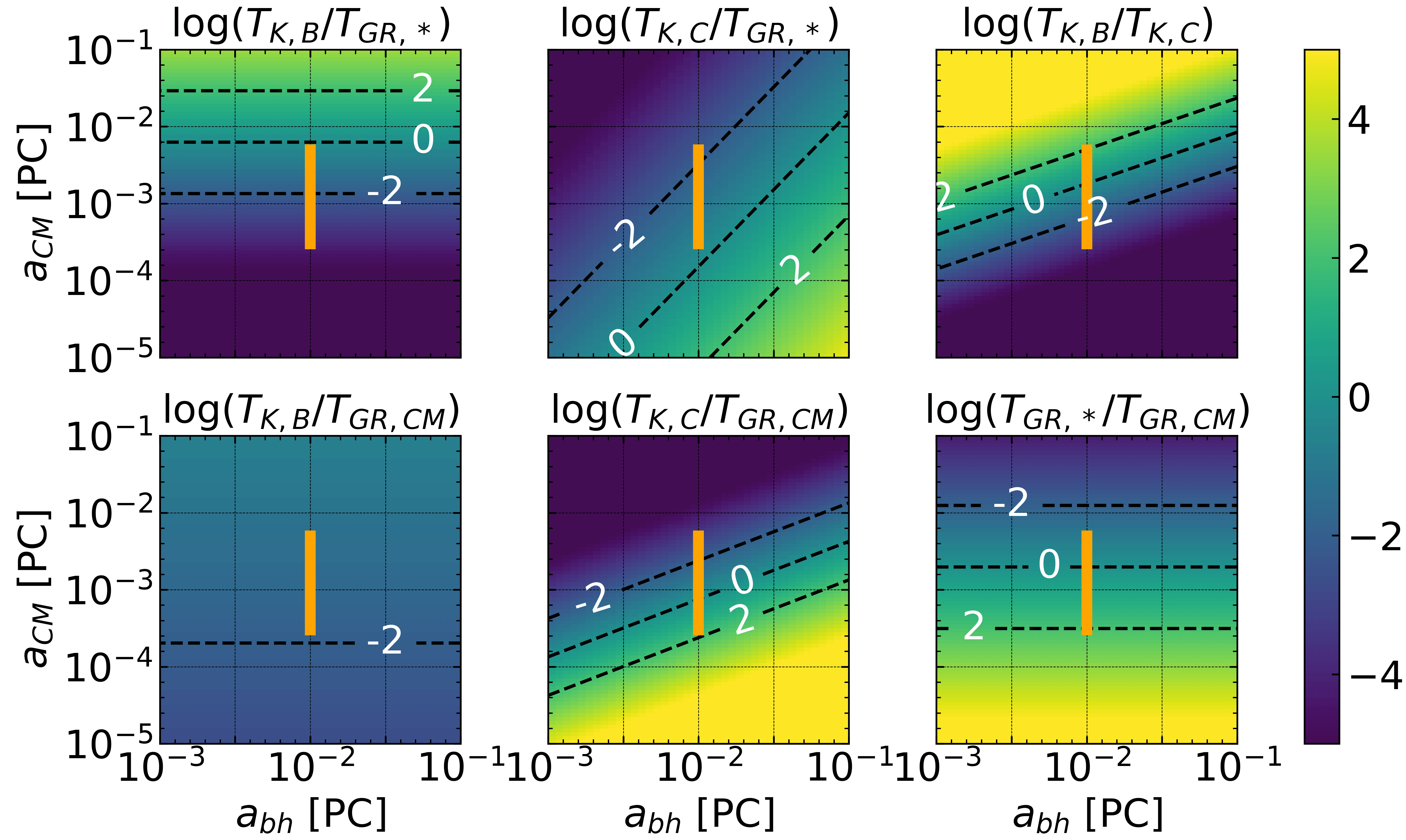
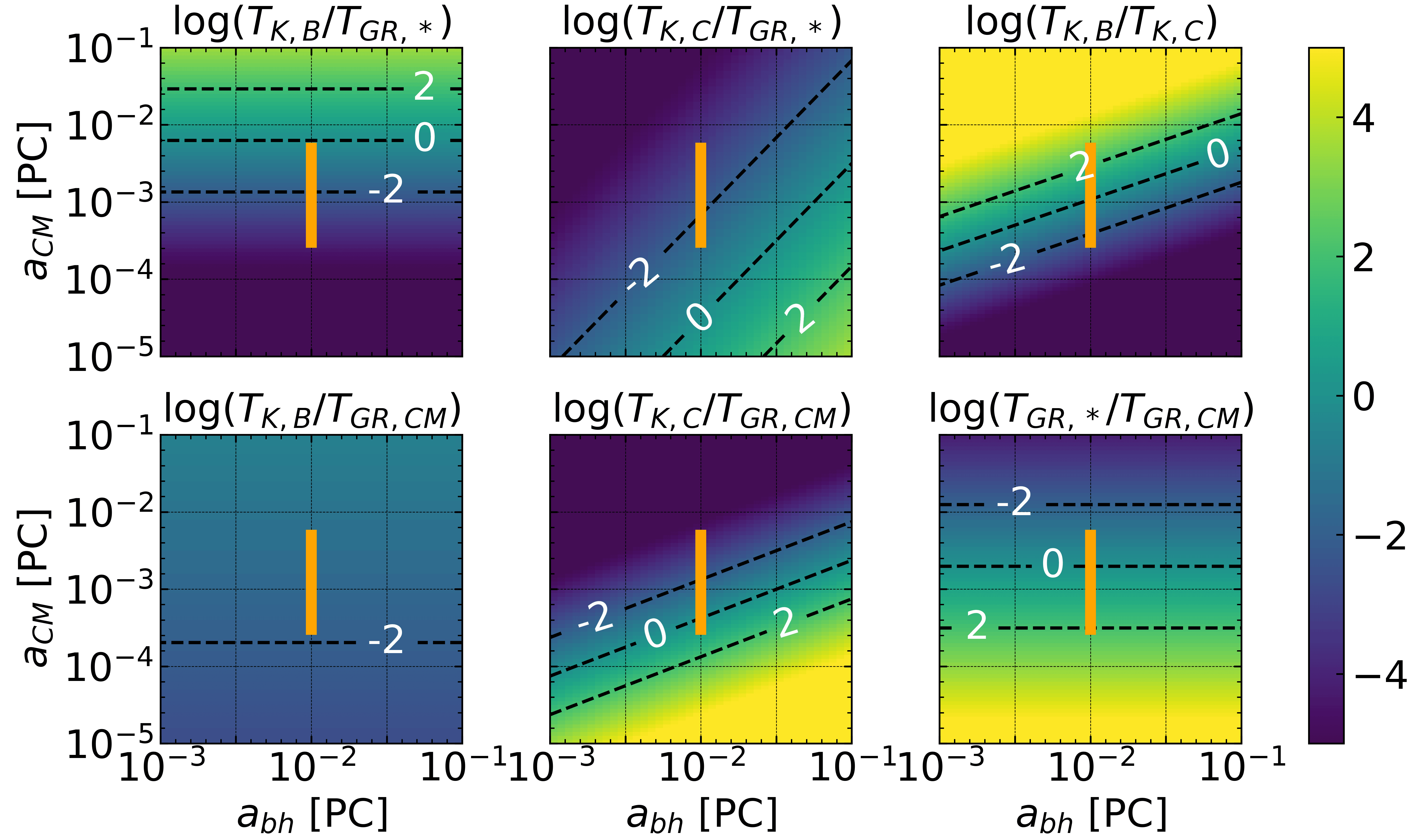
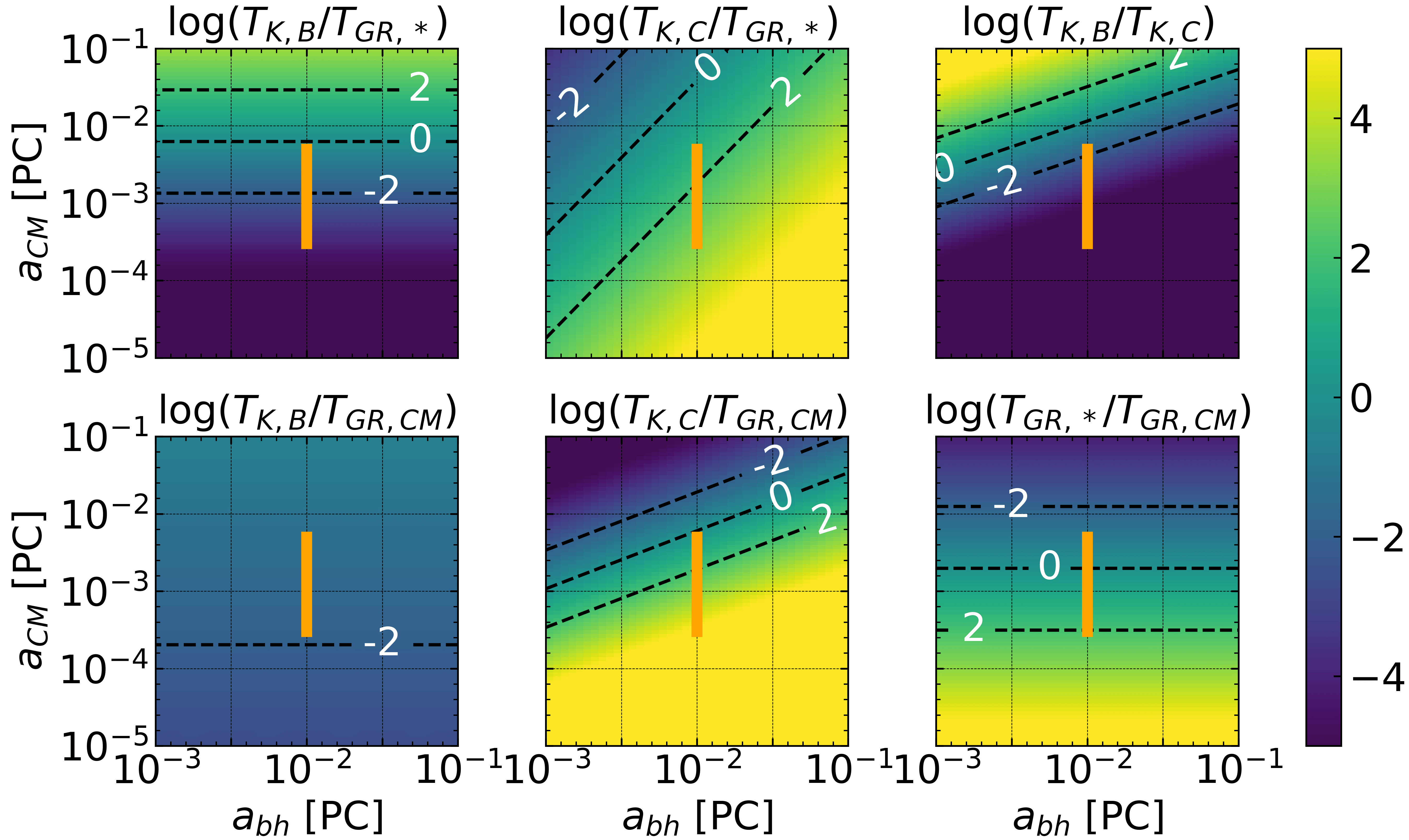
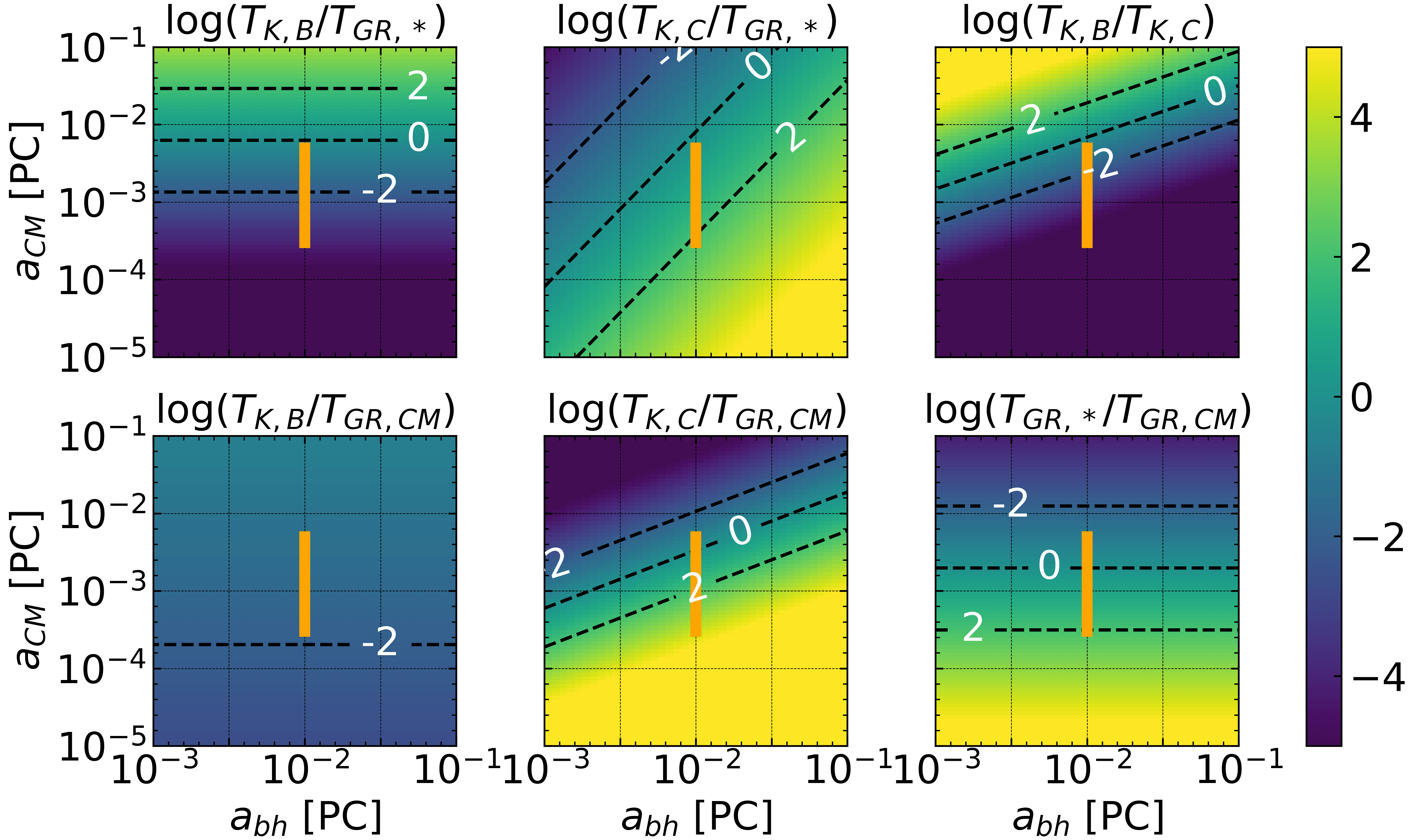
Figure 2 shows a comparison of the timescales in an illustrative example: , and with different sets of mass ratio and eccentricity of the binary SMBH.
We ran our simulations with input parameters indicated with orange lines in Figure 2. In this region, at , it is clearly shown in all four panels that both and are much longer than . This means that GR precession of the orbits is totally suppressed by the inner LK oscillations at any point in the parameter space we consider. Therefore, GR can be neglected in these simulations. The lower-middle inset in the lower two panels indicates that GR precession of the stellar binary centre of mass orbit dominates over the outer LK oscillations. Thus, for small mass ratios, post-Newtonian terms must be included in these simulations. The upper left-most inset in the upper two panels indicates that, for large mass ratios, the inner and outer LK oscillations compete with each other. This can serve as a catalyst for the occurrence of a number of interesting astronomical events, such as TDEs, HVSs and mergers. Conversely, in the lower two panels with small mass ratios, the outer LK oscillations are completely suppressed by the inner LK oscillations. In this case, stellar mergers become the dominant event in our simulations.
 |
 |
 |
 |
3 INITIAL MODELS AND NUMERICAL METHODS
In this section, we describe the numerical method used in this paper, and present the orbital parameters and initial conditions considered for the target four-body system.
3.1 Numerical Method
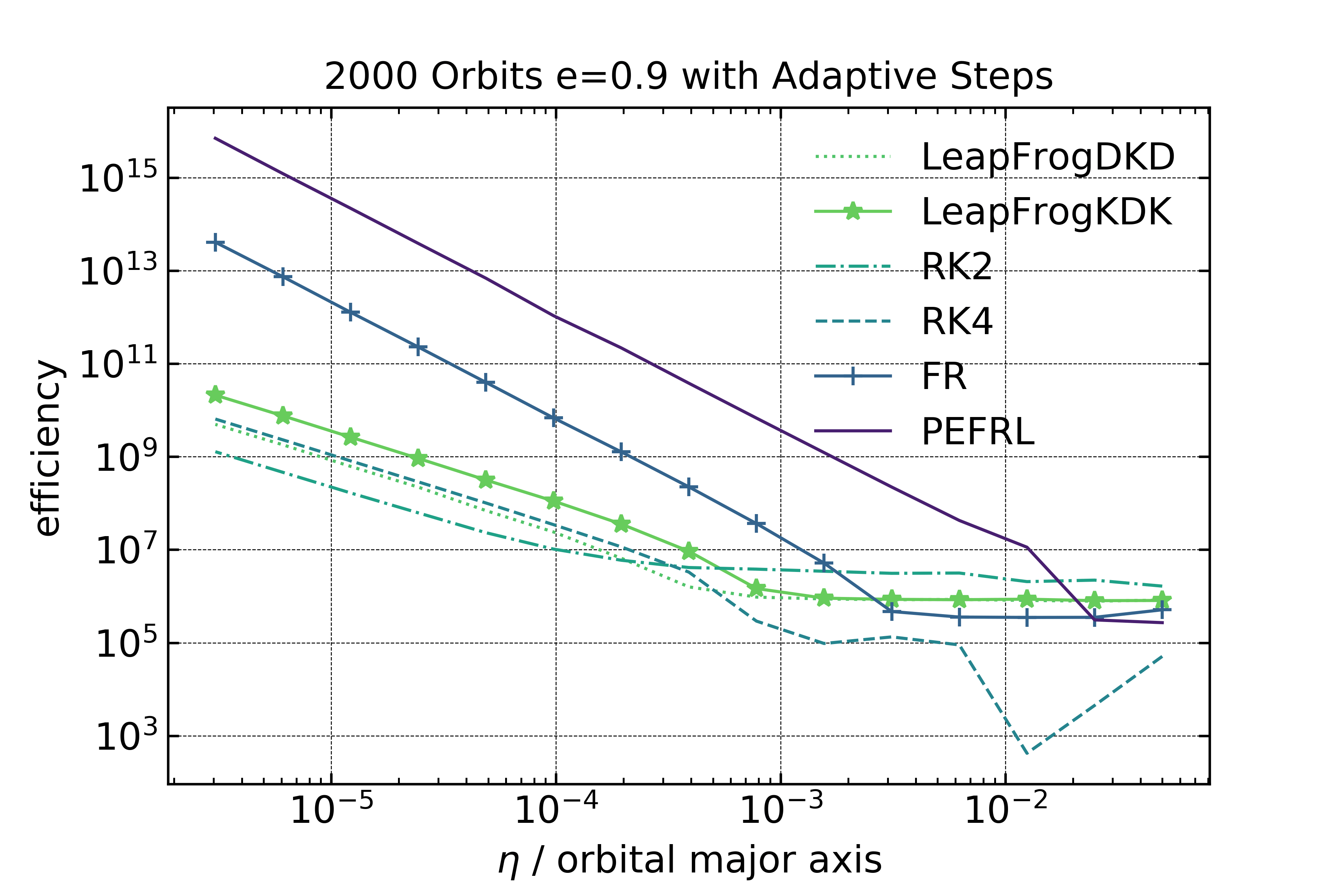
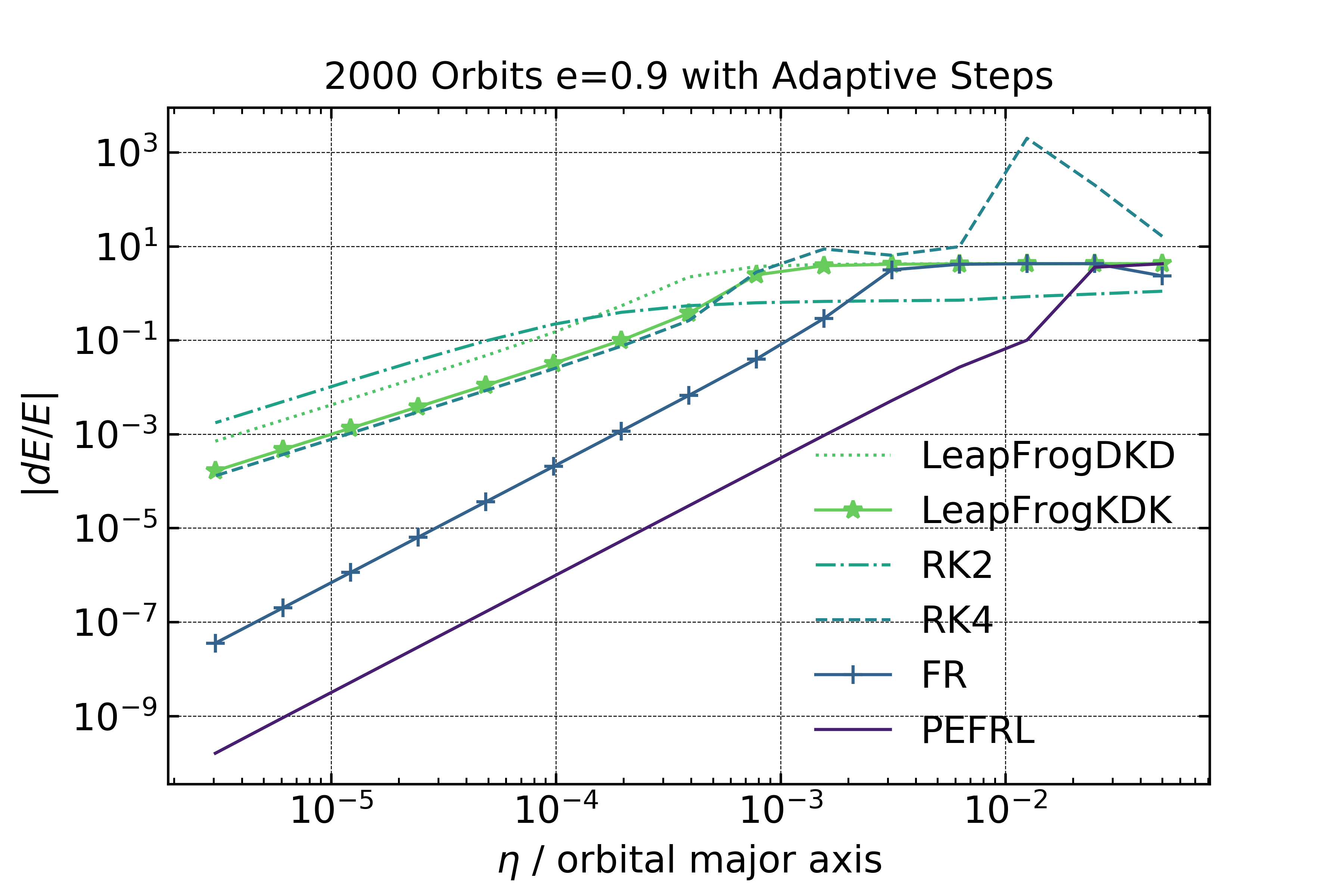
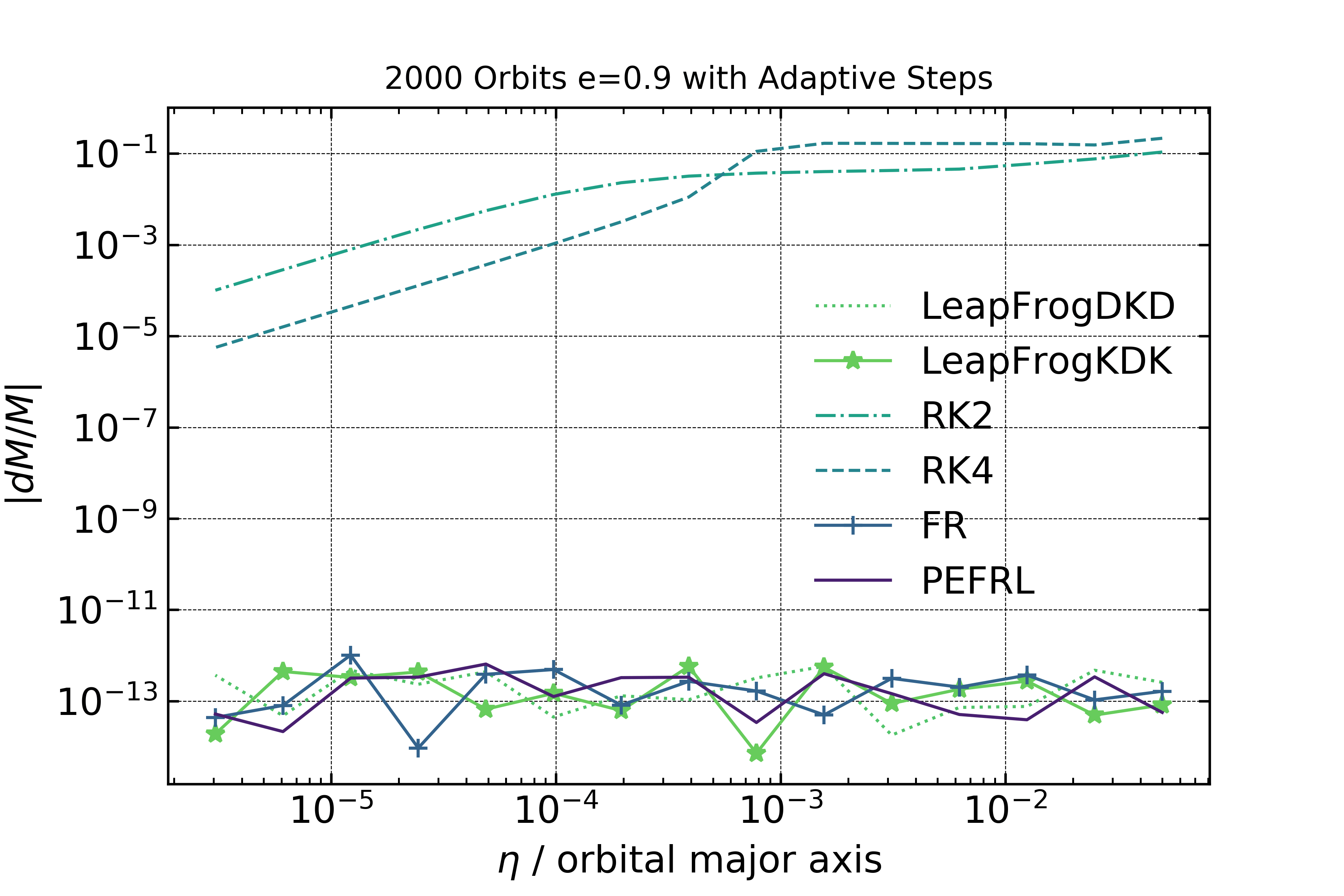
We use -body simulations to study the evolution of main sequence binaries in the Galactic Centre. In each simulation, a stellar binary orbits the central SMBH, which is in turn orbited by a remote less-massive SMBH. All the simulations were carried out using the code NBODY, developed by ourselves. In this code, we use the Position Extended Forest-Ruth Like (PEFRL) integrator with adaptive time stepping. The PEFRL algorithm is a fourth-order symplectic numerical method. Unlike other algorithms, the symplectic method conserves the constants of motion (i.e., total energy E and total angular momentum L) in Hamiltonian systems over long integration times. We test the performance of several integrators using our -body code by adopting the same set of initial conditions, performing the same simulations and comparing the results. As expected, symplectic methods perform better than non-symplectic methods (see the Appendix A for more details).
To ensure reasonable integration times, we do not use the regular adaptive time stepping control strategy, since this requires the higher-order error estimation embedded in the PEFRL algorithm. Instead, we adopt the time-step criterion in the cosmology code GADGET-2(e.g., Springel, 2005):
| (11) |
where is the minimal time-step allowed in the system, to avoid an infinite shrinking of the time-step. is an user-chosen accuracy parameter and gives the minimal acceleration among all the particles in the system at any given time . This time-step criterion is only dependent on the current status of the system. Thus, additional integration time is not needed to perform higher-order estimations. In our chosen problem, given the initial total energy of the system , the PEFRL method controls the energy fluctuation to remain within the range - , assuming .
The equation of motion is determined by the Newtonian gravitational acceleration, including post-Newtonian terms up to 2.5th order
| (12) |
where is the Newtonian acceleration imparted to the i-th particle
| (13) |
and above is the direction vector.
Post-Newtonian terms up to 2.5th order (Soffel, 1989) are included in the equation of motion in those areas of parameter space in Fig.2 for which the effects due to GR are important. Otherwise, we set to zero in our simulations.
| (14) |
where , and represent the 1st-order, 2nd-order and 2.5th-order terms, respectively(e.g., Kupi, Amaro-Seoane, & Spurzem, 2006). Since the full equation is very long, we are not going to expand it here.
3.2 Initial conditions and orbital parameters
We chose the mass of the primary SMBH to be , and investigated the mass ratio of the SMBH-SMBH binary in the range at [1/2,1/4,1/8,…,1/4096]. The mass of the stars in the stellar binary are both set to be .
The initial conditions of our restricted four-body problem are then completely defined by ten configuration parameters: three for the SMBH-SMBH binary, three for the orbit of the binary star about the primary SMBH and four for the binary star itself. These are:
-
1.
the inclination between the SMBH binary orbit and the binary star orbit, ;
-
2.
the longitude of the second black hole’s ascending node, ;
-
3.
the argument of the second black hole’s pericenter, ;
-
4.
the semi-major axis of the centre of mass of the stellar binary, ;
-
5.
the specific angular momentum of the centre of mass of the stellar binary, ;
-
6.
the mean anomaly of the centre of mass of the stellar binary, ;
-
7.
the inclination of the binary star’s inner orbit relative to its center of mass orbit, ;
-
8.
the longitude of the stars’ ascending node in the stellar binary, ;
-
9.
the argument of the stars’ pericentre in the stellar binary, ;
-
10.
the mean anomaly of the stellar binary, .
For an isotropic stellar distribution, we sample randomly in the range [-1,1], and and randomly in the range [0,2]. is sampled randomly in the range [0.03,0.5], while is evenly sampled in the range [-1,1]. All other phase parameters of the binary star are sampled randomly in the range [0,2]. The other two configuration parameters, namely the eccentricity of the stellar binary (set to 0) and the eccentricity of the SMBH binary (set to [0.3,0.5,0.7] ), are fixed in each group of simulations.
We run 10,000 experiments for each group of input parameters, with an integration end-time of . In each experiment, particles are deleted from the simulation upon entering either the tidal disruption radius or the event horizon of either SMBH. Similarly, if a particle escapes to a distance from the primary SMBH, then the particle is also deleted. A merger event occurs when the distance between two particles becomes less than the sum of their radii. We treat the merger as a completely inelastic collision, hence we delete both particles and create a new particle at the centre of mass. All events - TDEs, mergers and escapes/HVSs - are recorded until either the maximum integration time is reached or only two particles remain in the system.
4 Numerical exploration of the four-body system
4.1 Classification of the simulation results
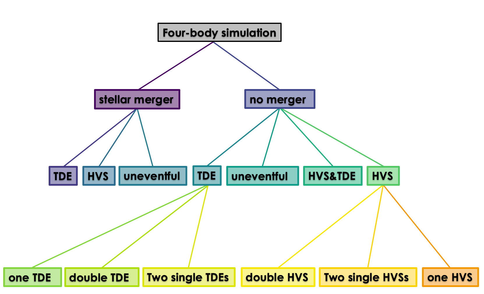
Four types of events are recorded in our four-body simulations. These are TDEs, breakup of stellar binaries, mergers and HVSs. Compound events are made up from these four basic events. For example, two TDEs occurring sequentially within a short time interval make a double TDE. Two HVSs without the breakup of the stellar binary make a double HVS. Binary disruption with a TDE makes a pure single TDE. And so on. In total, there are 11 kinds of compound events.
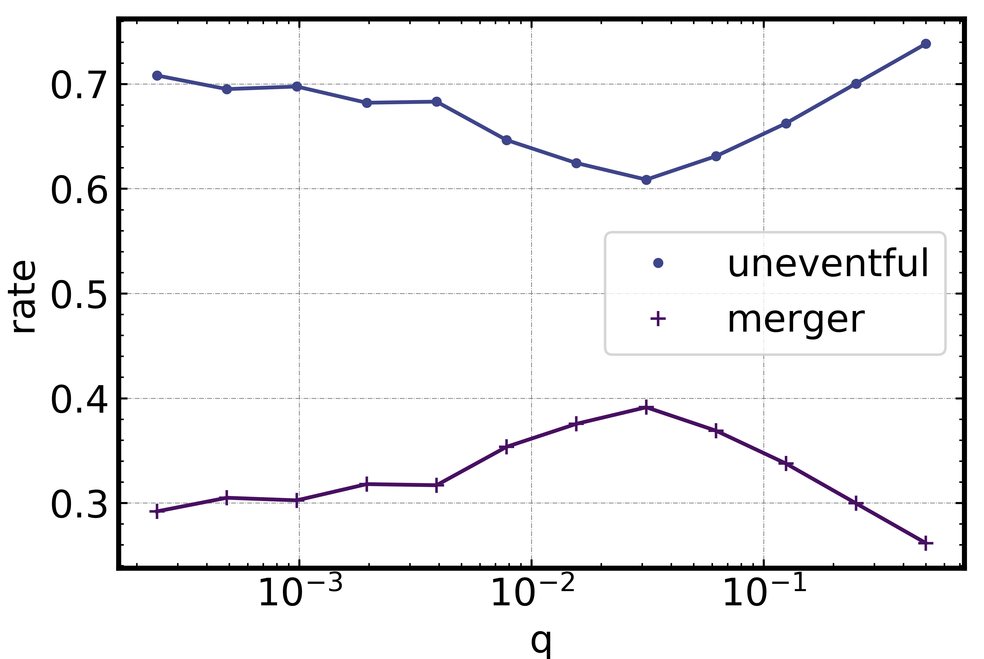
As shown in Fig.3, we organize the events into a tree structure. At the top root, we perform our simulations with the initial conditions given in Section.3.2. The first level distinguishes between simulations with a binary merger and those without. Once a merger occurs, the four-body system changes into a three-body system. The subsequent evolution of this three-body system, including the formation of TDEs and HVSs, have been well studied. If no merger occurs, a richer set of outcomes are possible relative to the single star case. The additional star makes the second level branch of our tree possible. At the second level branch, the outcomes are TDE, HVS, HVS with TDE and uneventful. At the third level, the TDE (HVS) classification is divided into one and two TDEs (HVSs). However, due to the breakup of stellar binary, the two TDE (HVS) case can also be divided into two single TDEs (HVSs) and a double TDE (HVS). The distinction here is the bound status of the stellar binary at the moment of occurrence of the event. The event rates of the branches at a given level or node of the tree always add to unity.
4.1.1 Binary star mergers
Binary star mergers are predominantly caused by orbital eccentricity excitation from LK oscillations in the inner triple system. LK oscillations at the quadrupole level keep the semi-major axis of the orbit constant, such that an increase in the eccentricity leads to a decrease in the pericentre distance . Once the pericentre is sufficiently small, the two stars collide with each other. The critical distance for this to occur is defined as the sum of the radii of the two stars. Therefore, the merger criterion is
| (15) |
The stellar radii and are calculated from the mass-radius relation (e.g., Hansen, Kawaler, & Trimble, 2004). The initial is set to 0.1 and the stellar binary has a total mass set equal to 3 in our simulations. Therefore, the critical eccentricity for merger is .
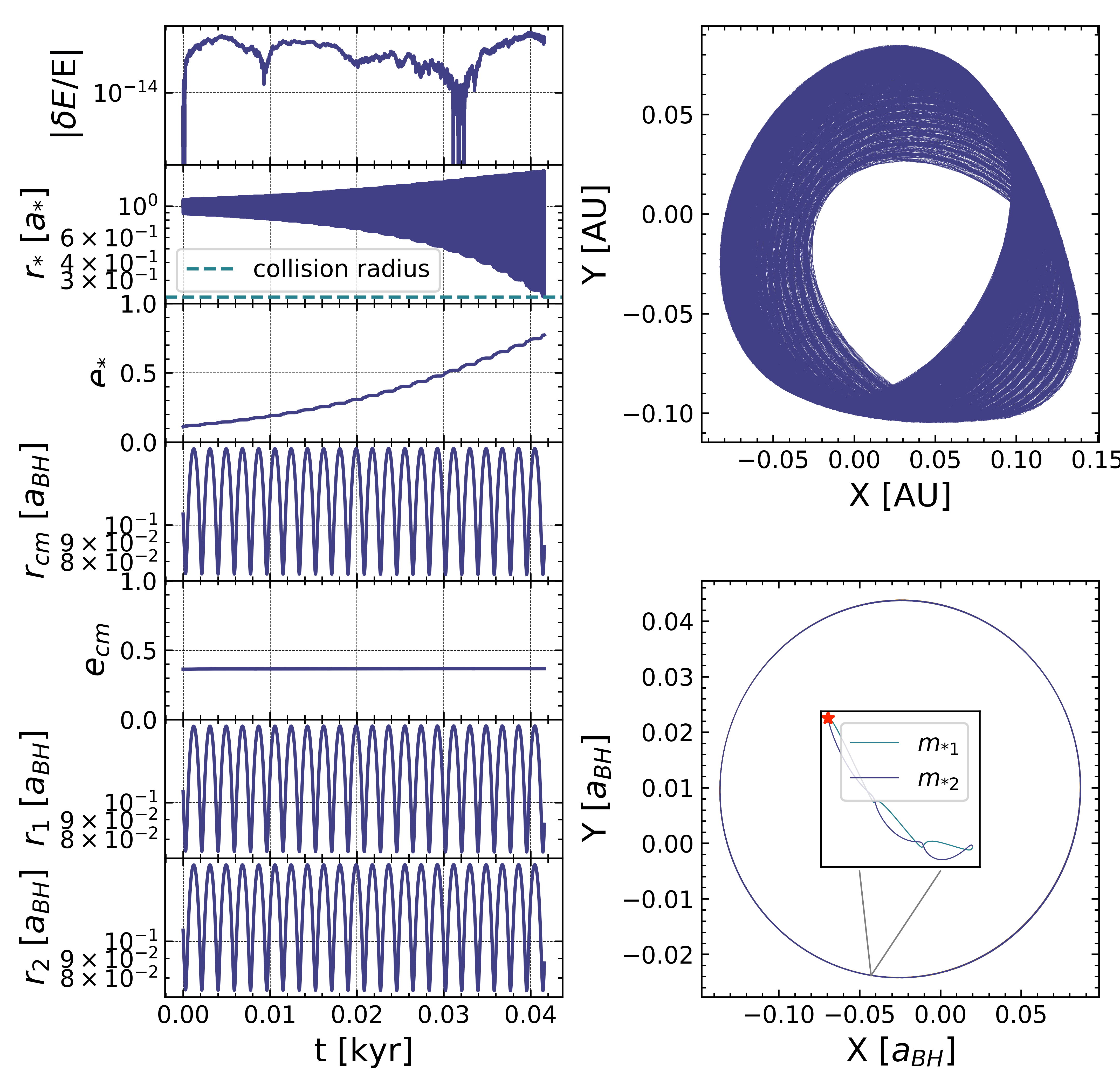
As we discuss in Sec.2.2, for our chosen initial conditions, the time scale for relativistic precession of the inner binary orbit is much longer than . We do not include dissipative tidal forces in our model. Therefore, the two main mechanisms for suppressing the LK oscillations and reducing dramatically the orbital separation in the case of mergers (Prodan, Antonini, & Perets, 2015) cannot operate. Figure 4 shows an illustrative example of a merger in our simulations. In this example, the inner inclination is larger than the critical angle required for LK oscillations, such that the inner LK oscillations excite the eccentricity of the stellar binary orbit until reaches the critical collision distance. The outer inclination is smaller than the critical angle, such that the outer LK oscillations are completely suppressed. Therefore, stays the same through the simulation. It is clear in this example that the outer LK oscillations are totally suppressed by the inner LK oscillations. The outer LK oscillations can be absolutely suppressed if , or by the initial orbital inclination of the outer triple falling out of the range , where . From Eqs.6,7 and Fig.2, we speculate that most merger events occur in the inner region (small initial ) around the SMBH where is dominant. For those merger events that occur in the outer region (i.e., with large initial ) where , the outer LK oscillations are stifled by the small inclination . In this way, the inner LK oscillations dominate and finally lead to a stellar merger on a longer timescale compared to at smaller initial .
4.1.2 Tidal Disruption
Tidal disruption is caused by orbital eccentricity excitation in the outer triple system. The perturbation from the secondary SMBH causes the binary star to migrate in closer to the SMBH. Once the binary star reaches the stellar tidal disruption radius , a TDE occurs. However, due to chaotic perturbations to the binary star, the condition for a stable triple system in Eq. 4 is not upheld in all regions around the primary SMBH. In the region where the triple system remains stable, outer LK oscillations play a fundamental role in exciting the orbital eccentricity. Outside the stable zone, other chaotic dynamical effects can also excite the orbital eccentricity.
If the stellar binary resides in the stable three-body region, LK oscillations become the main mechanism for producing TDEs. From Eq.1, the condition for a TDE is,
| (16) |
For an SMBH mass , for a star is . In our simulations, the semi-major axis of the SMBH binary is 0.01, and the centre of mass of the binary star is sampled evenly between . This yields the typical eccentricity for a TDE .
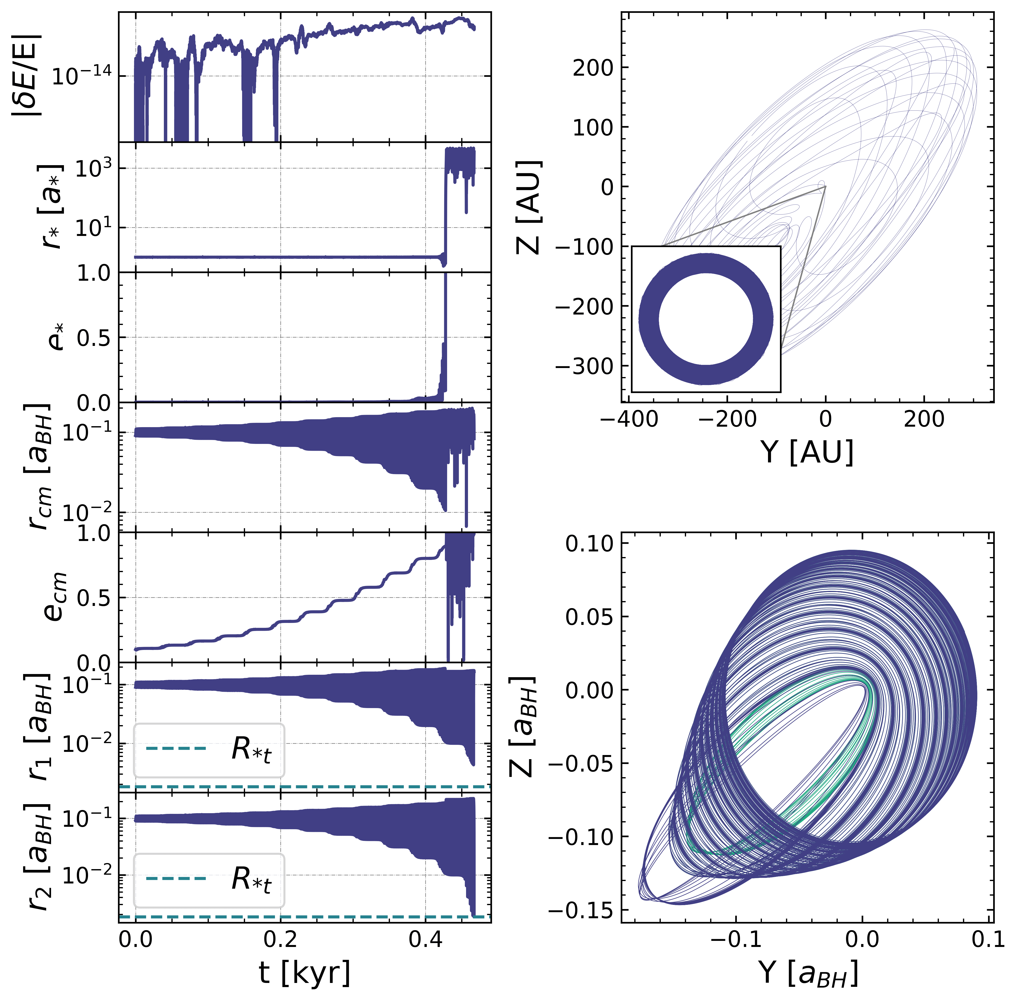
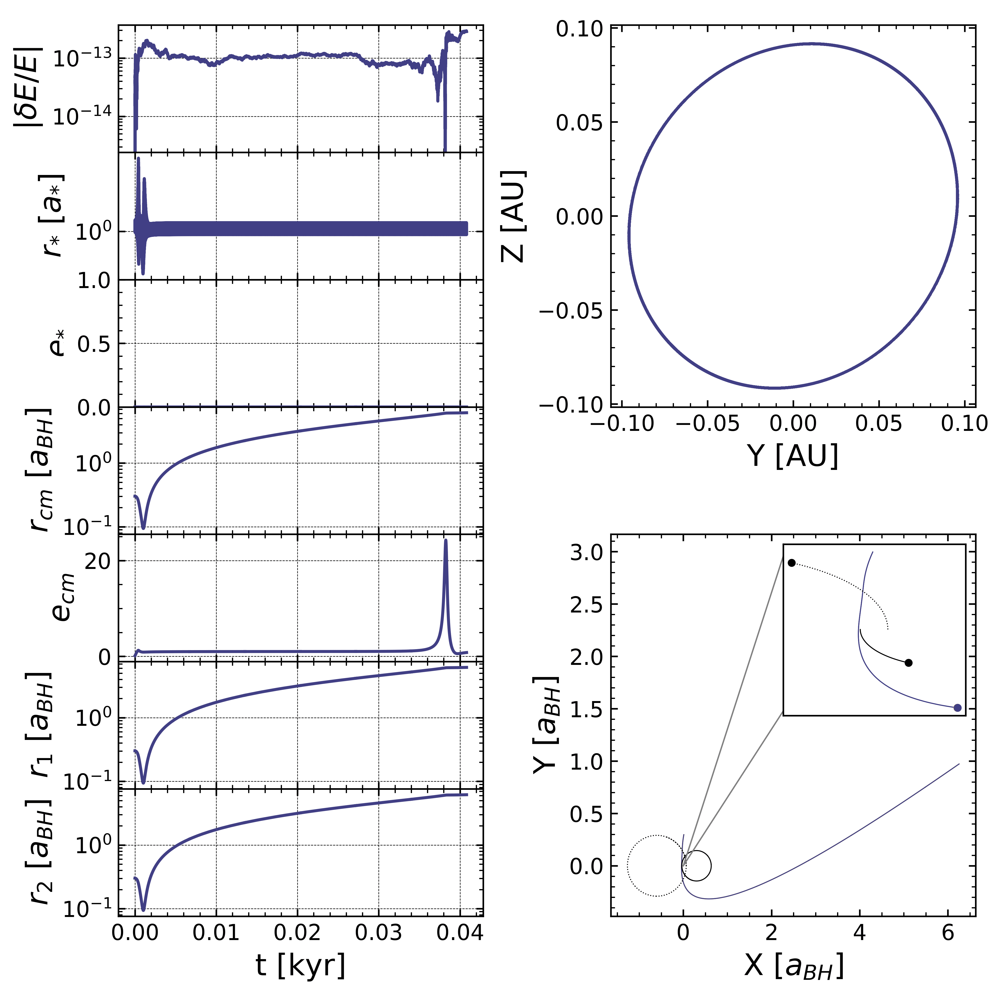
Figure 5 shows an illustrative example of a TDE from LK oscillations. In this example, the outer inclination is larger than the critical angle, such that the outer LK oscillations excite the eccentricity of the binary star’s centre of mass . The inner inclination is smaller than the critical angle for LK oscillations , such that the inner LK oscillations are totally suppressed. The binary star maintains a perfectly circular orbit with constant until around 0.41 kyr, at which point the stellar binary is disrupted due to the tidal force exerted by the primary SMBH . After this decoupling, the two stars remain in orbit about the primary SMBH. The outer LK oscillations continue to excite the stars’ orbits until a single TDE occurs. Unlike for binary mergers, the inner LK oscillations need to be suppressed by the outer LK oscillations in order for a TDE to be produced. The inner LK oscillations can be suppressed either if , or if the initial orbital inclination of the inner triple falls outside of the range for LK oscillations . From Eqs.6,7 and Fig.2, we conclude that is always smaller in the outer region around the SMBH. Therefore, for binary stars with initial semi-major axis in this area, TDEs occur more frequently than HVSs. TDE events can also occur in the inner region around the SMBH, but only if the binary’s orbit is nearly coplanar with the orbit of the binary centre of mass about the SMBH. In this case, the inner LK oscillations that drive stellar mergers cannot be activated due to the low inclination . The maximum eccentricity that can be induced by LK oscillations is constrained by the initial inclination . The high eccentricity needed for TDEs ([0.99,0.999]) requires that the orbital plane of the binary centre of mass about the SMBH be nearly perpendicular to the binary’s orbital plane.
If Eq. 4 is not satisfied, the system becomes chaotic. Chaotic effects could also excite the eccentricity (e.g., Chen et al., 2009). Unlike quadrupole LK oscillations, chaotic effects do not conserve the semi-major axis of the orbit. Consequently, the subsequent evolution can be difficult to predict. However, the simulation results allow us to study chaotic excitations statistically.
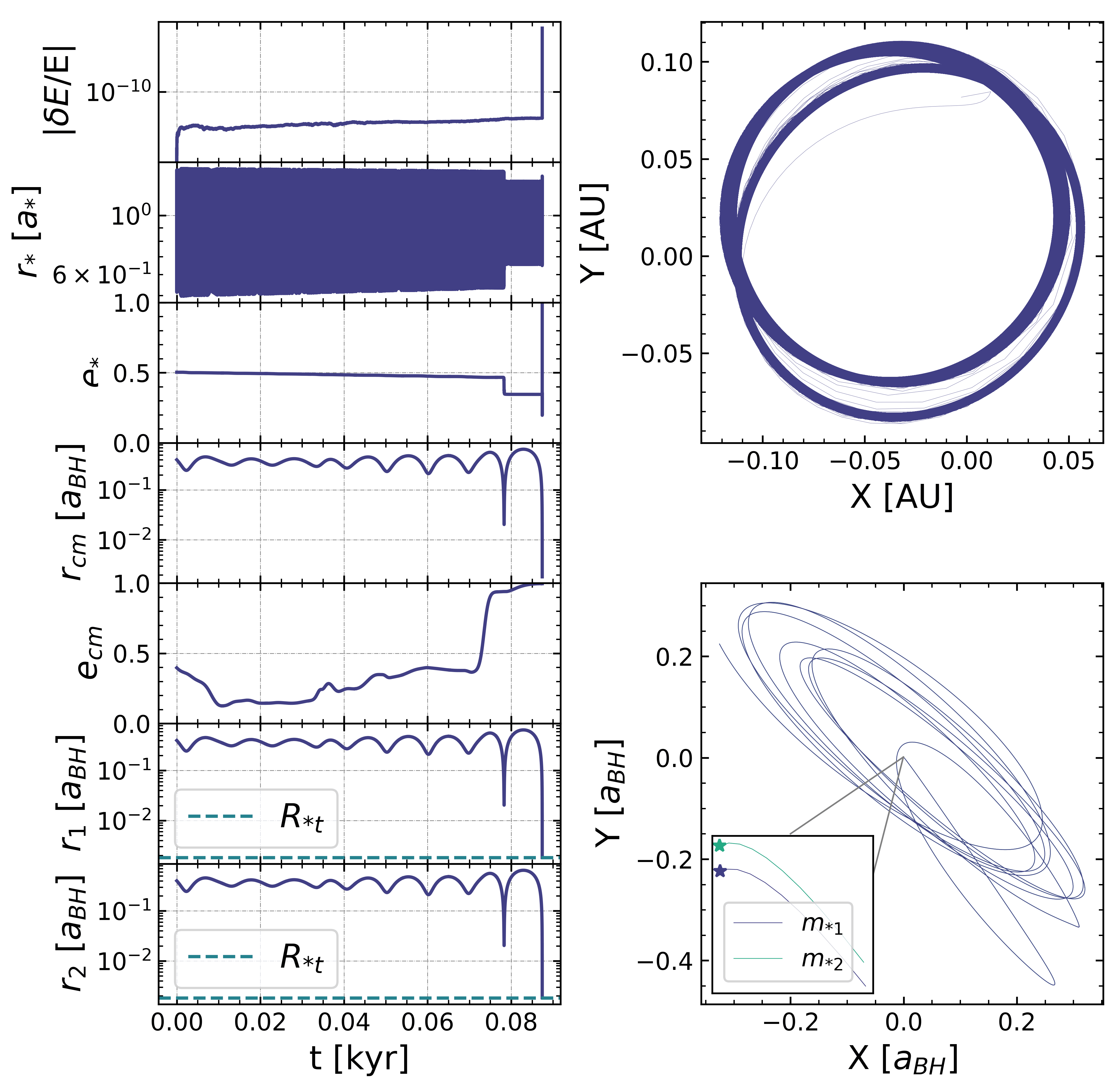
Figure 6 shows an illustrative example of chaotic excitations. The stellar binary maintains an almost elliptical orbit at the beginning of the simulation. The first close encounter with the SMBH, which occurs around 0.08 kyr, causes the stellar binary to become more compact. At the same time, the eccentricity of the centre of mass of the stellar binary’s orbit about the SMBH is suddenly excited. This excitation leads to an extremely high eccentricity, which subsequently produces a double TDE during the second close encounter.
4.1.3 Hypervelocity Stars
Hypervelocity stars can be produced by the slingshot effect (Lu, Yu, & Lin, 2007), or the interaction between a globular cluster and an SMBH/SMBHB(Capuzzo-Dolcetta & Fragione, 2015; Fragione & Capuzzo-Dolcetta, 2016; Fragione, Capuzzo-Dolcetta, & Kroupa, 2017). In our simulations, most binary stars remain within the Hill sphere of the primary SMBH. In a stable hierarchical triple system, LK oscillations cannot produce HVSs because they conserve the semi-major axis of the orbit. However, if we replace the single star in a triple system with a stellar binary, the binary can be disrupted at the tidal breakup radius of the stellar binary , which re-distributes energy and angular momentum within the four-body system. This energy and angular momentum re-allocation can produce HVSs.
Figure 7 shows an illustrative example of a double HVS. The inner inclination is smaller than the critical angle, such that the inner LK oscillations are suppressed. The outer inclination is larger than the critical angle. Therefore, the outer LK oscillations should result in an excitation of the orbit of the centre of mass of the stellar binary. However, since , and , the secondary SMBH gets very close to the stellar binary, leading instead to an ejection event. The distance to the SMBH of the stellar binary is insufficiently small for it to be disrupted after a slight oscillation, and a double HVS occurs instead. Most HVSs are the result of a strong perturbation from the secondary SMBH, which occurs most frequently for larger mass ratios and higher eccentricities . Such a strong perturbation can even result in a double HVS event.
4.2 Event rates for different SMBH binary mass ratios
LK oscillations in the inner and outer triple, together with non-secular effects and chaotic effects, influence the orbital evolution of the main sequence binary. The efficiency of the inner and outer LK oscillations depends on the relative ratio of their respective time scales. As Eq. 6 and 7 shown, the relative time scales of the inner and outer LK oscillations are sensitive to the ratios and . In our simulations, we fix the semi major axis of the stellar binary to reduce the free parameters in our model. Regardless, how a? affects the outcome is readily apparent from our simulations. When the inner LK oscillations dominate, the fraction of stellar mergers becomes large (as shown in Fig.11). In this case, the choice of binary mass and semi-major axis will affect the merger rate significantly. If the semi-major axis of the SMBH-SMBH binary and that of the stellar binary’s orbit about the primary SMBH are fixed, compact stellar binaries are harder to merger. This is because smaller values for yield longer time scales for the inner LK oscillations to operate. On the other hand, when the outer LK oscillations dominate, the choice of binary mass and semi-major axis do not influence the TDE and HVS event rates significantly. Here, the stellar binary can effectively be regarded as a single particle.
The presence of a background gravitational potential could also affect the relative event rates. In particular, in the Galactic Centre, dim low-mass stars are not detectable, and it is not known if any contribute to the local potential in the immediate vicinity of the primary SMBH. Any contribution to the potential from gas and/or dust is also not included in our calculations. Naively, however, we expect these contributions to have a negligible effect on the results reported in this paper. Scattering experiments under the presence of a background potential were recently performed by (Ryu, Leigh, & Perna, 2017), and subsequently applied to the production of runaway and hypervelocity stars (Ryu, Leigh, & Perna, 2017).It was shown that, unless the potential is very deep, the outcome of the scattering experiment is not significantly affected.
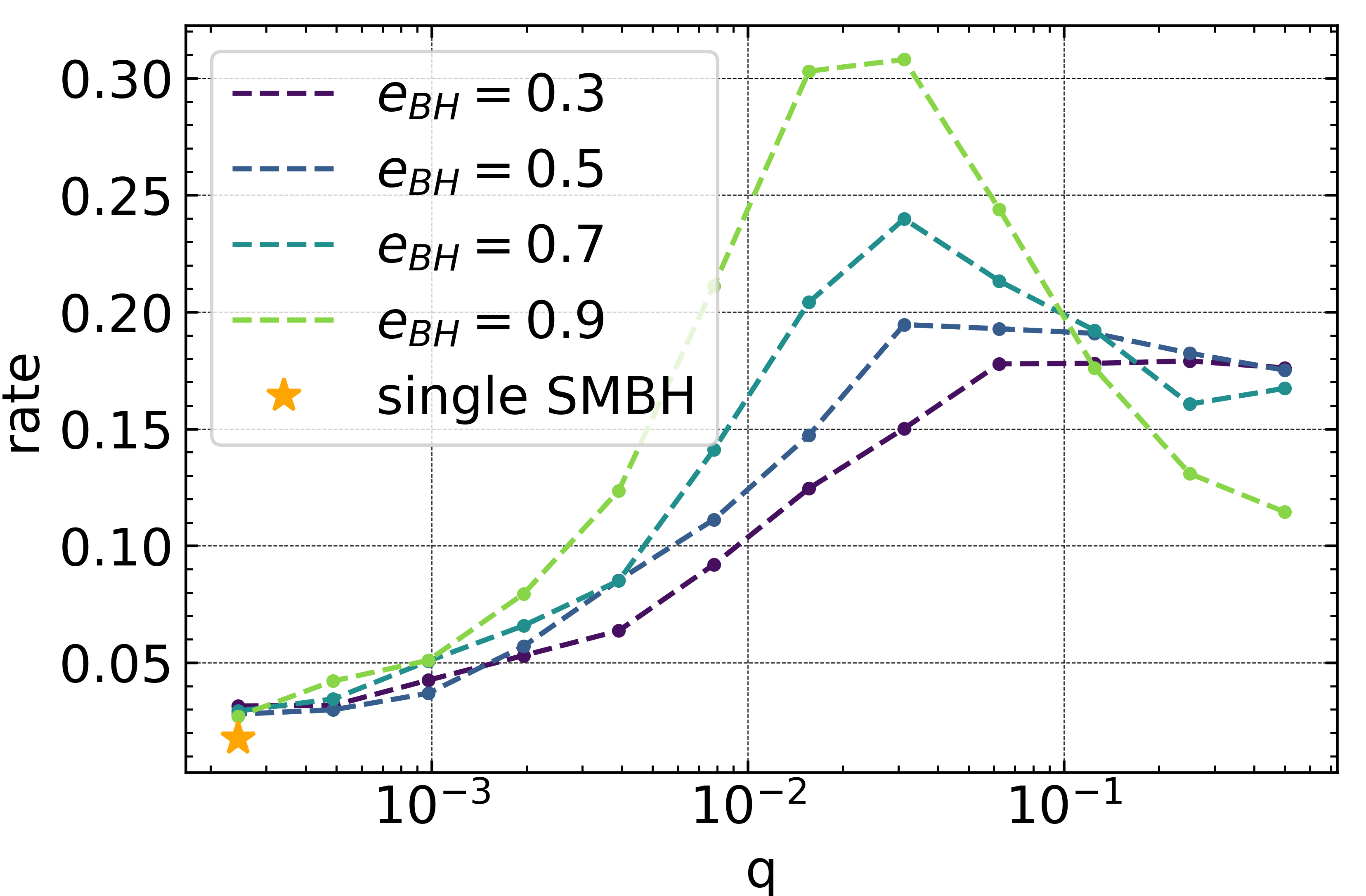
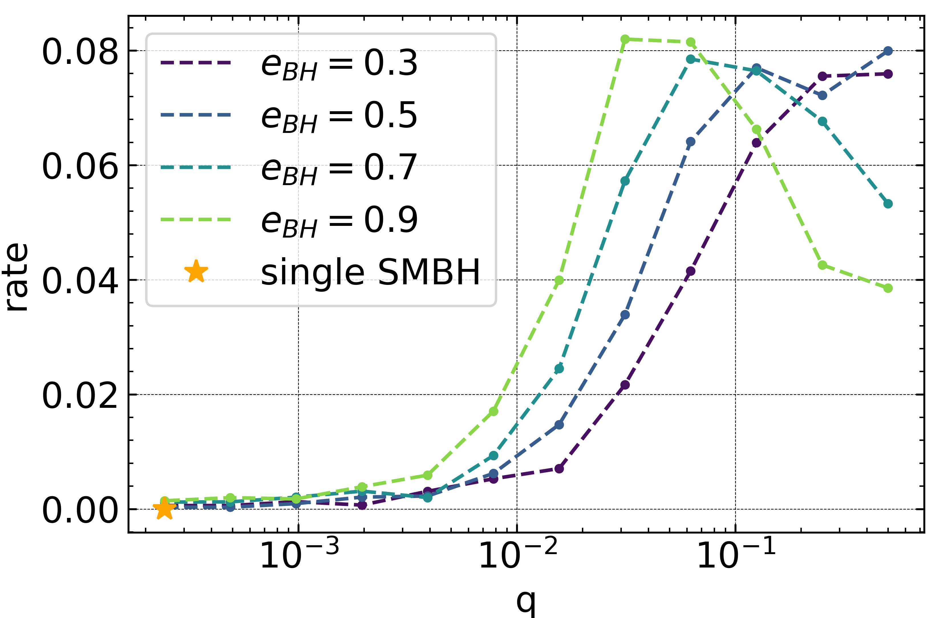
To quantify the significance of the secondary SMBH in deciding each outcome, we vary the mass ratio of the SMBH binary. Figure 8 depicts the rates of different events as a function of the mass ratio , for different eccentricities .
As the mass ratio increases, so do the total event rates. This is especially true for the double HVS rates. The TDE rates form a peak between and . The ’star’ at the left end of each curve shows the event rates for a single SMBH () obtained from three-body simulations. The event rates for the SMBH-SMBH binary converge to the single SMBH case when , except for single TDEs and single HVSs. The single TDEs (HVSs) come from the decoupling of the stellar binary, which is sensitive to the mass of the secondary SMBH. For the mass ratio , the mass of the secondary SMBH is still not small enough to neglect the effect on decoupling due to the secondary SMBH. Overall, the event rates for an SMBH-SMBH binary are always different than those obtained for a single SMBH. Consequently, the observed relative event rates can be used to constrain the possible presence of a binary SMBH companion orbiting the central primary SMBH in the Galactic Centre. We will return to this interesting possibility in Section 5.
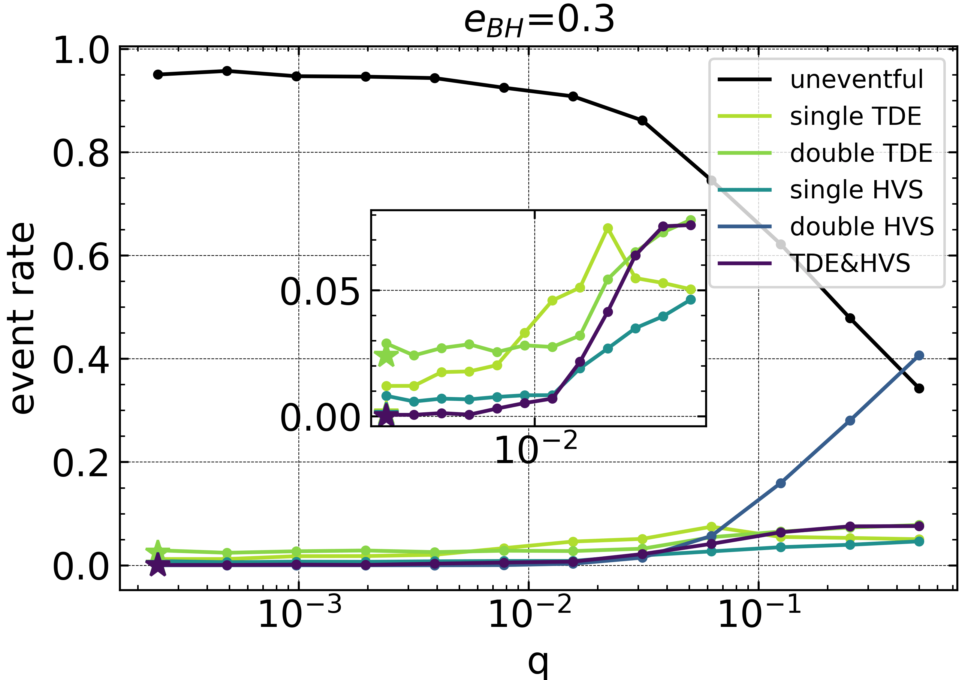
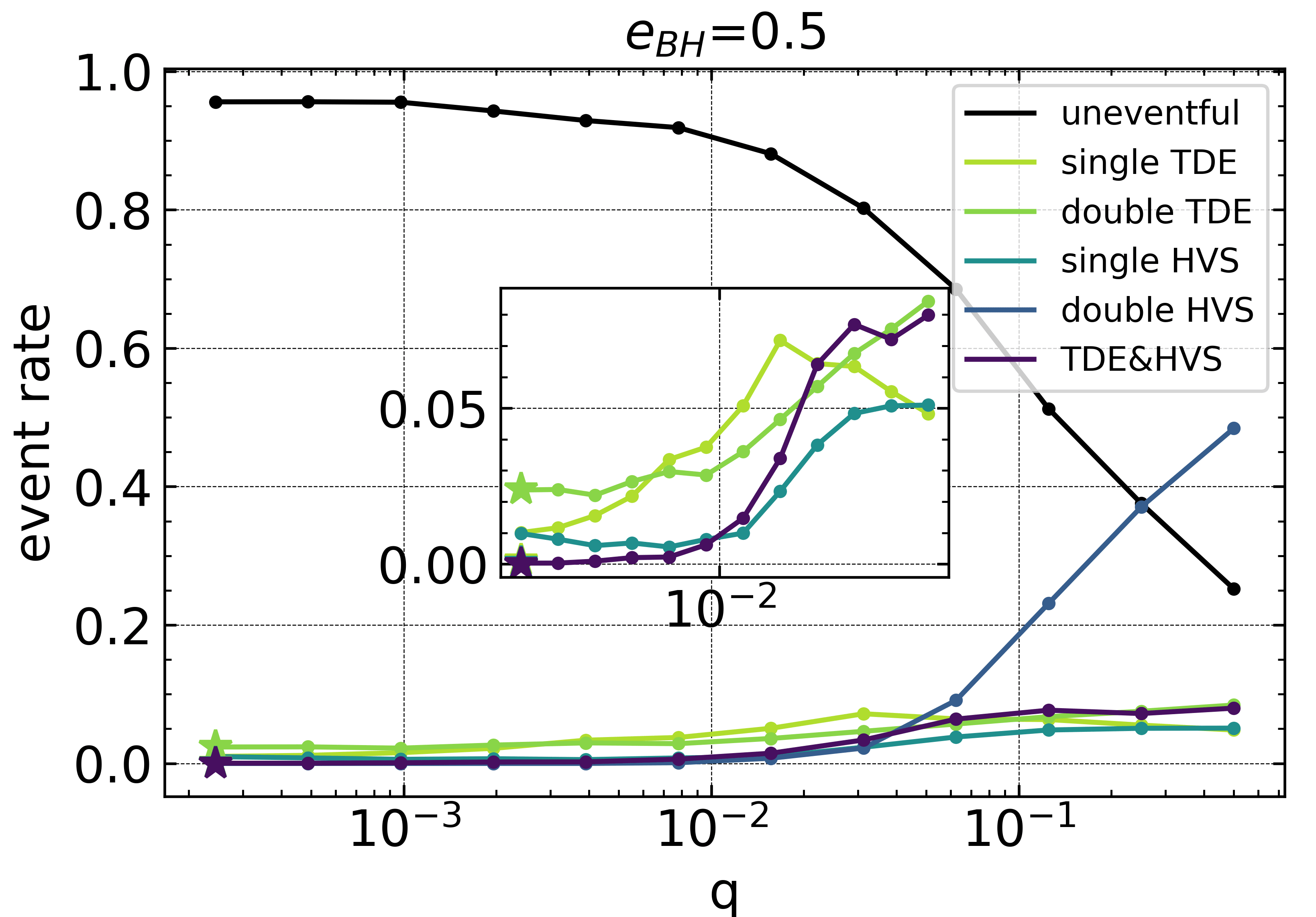
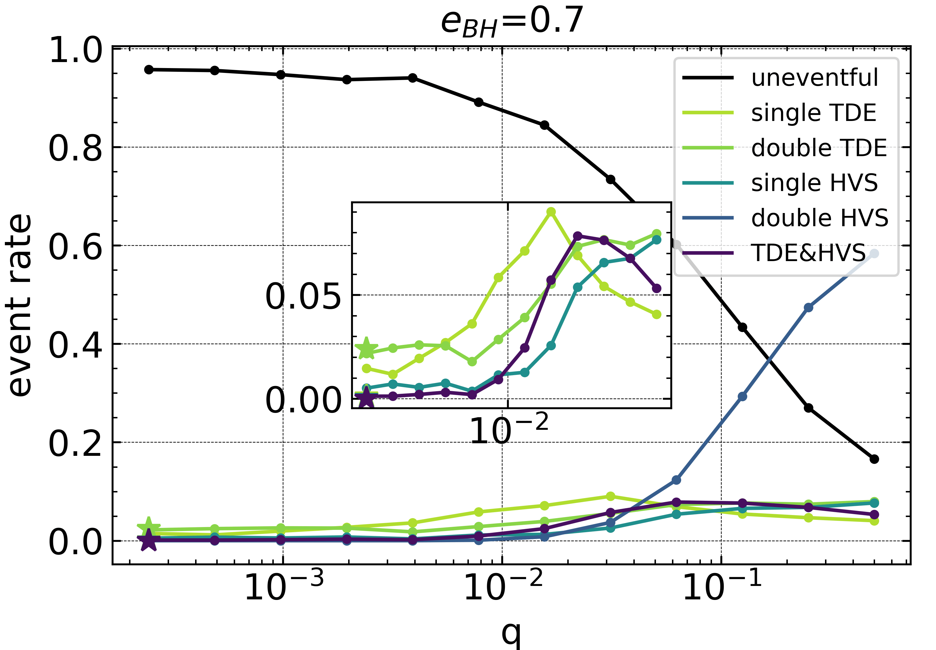
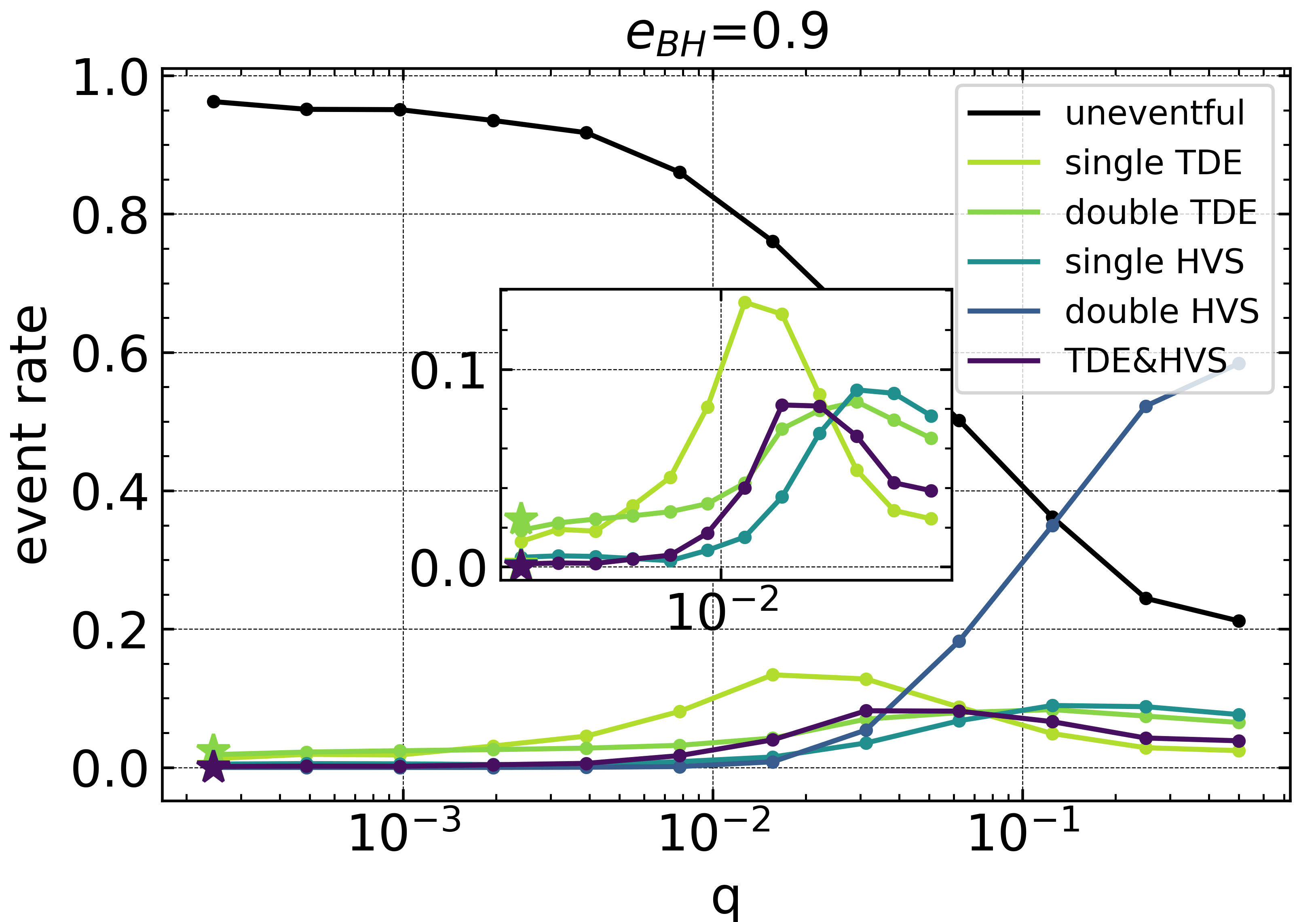
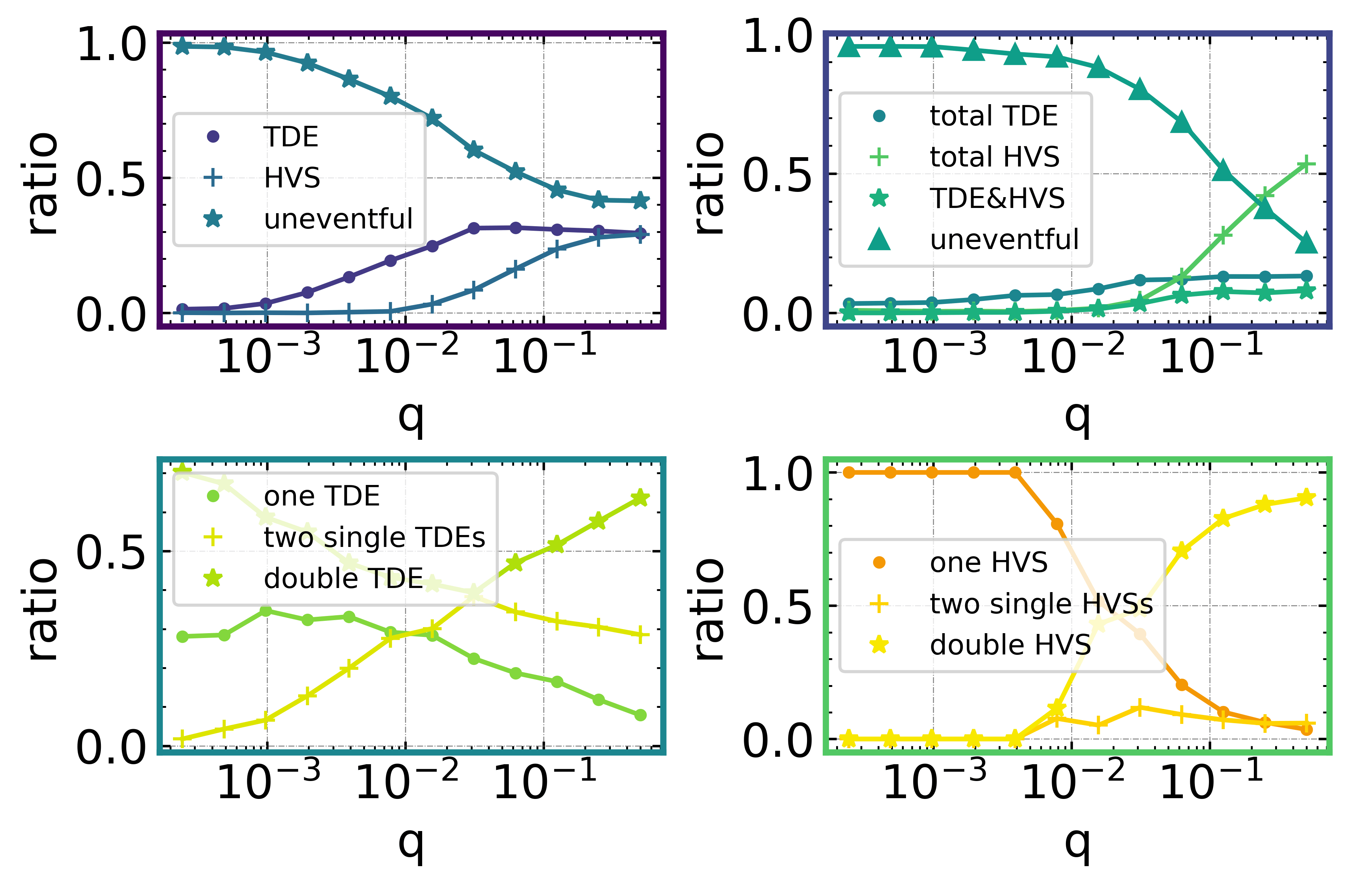
Figure 9 shows the relative rates for the different events shown in Fig. 3 for . Both the TDE and HVS rates increase with increasing mass ratio .
4.2.1 Merger Rate as a function of Mass Ratio
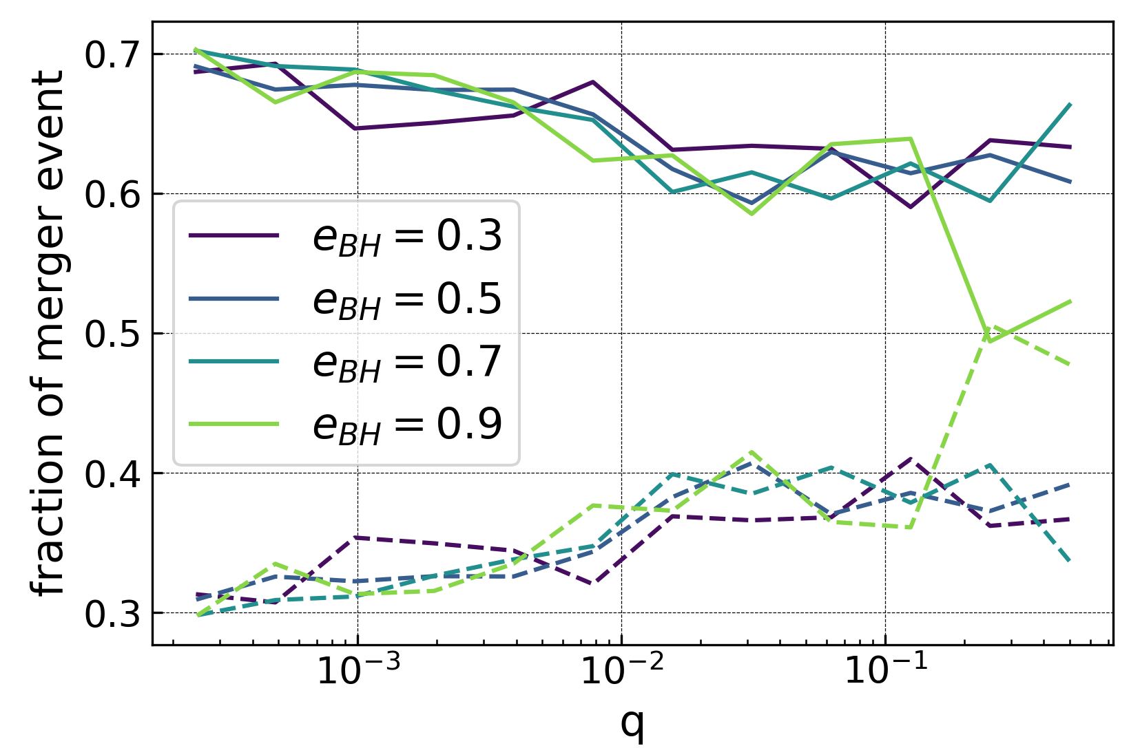
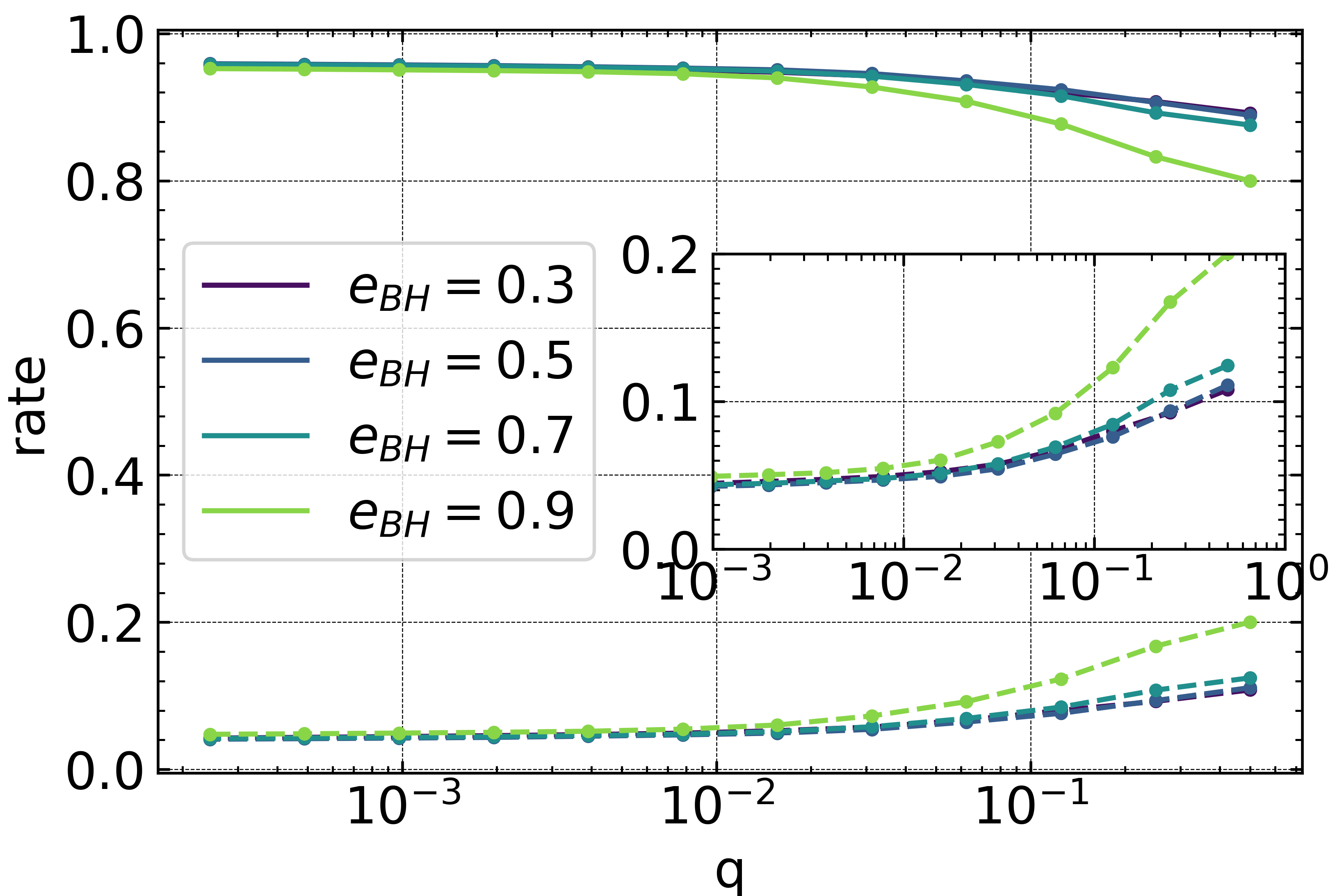
The most common event in our four-body system is stellar mergers. The merger events correspond to initial conditions for which the inner LK oscillations dominate. Fig.10 shows the fraction of merger events arising from different effects. We see that most merger events are due to LK oscillations. Therefore, the efficiency of the LK oscillations is what decides the dependence of the total merger rate on mass ratio . The upper panel of Fig. 11 shows the merger rates for different mass ratio. This mechanism should be independent of the mass of the second SMBH , since it is driven by the inner LK oscillations coming from the primary SMBH. However, the upper panel of Fig. 11 indicates that the merger rate increases slightly with increasing mass ratio. The reason for this slight increase is that the inner and outer LK oscillations are not completely independent. In regions where both the inner and outer LK oscillations affect the stellar binary, the outer LK oscillations could excite the stellar binary to migrate in closer to the primary SMBH , where the inner LK oscillations are stronger, leading to higher merger rates. The peak of the merger rate appears between and . Above the peak mass ratio, the merger rate starts to decrease due to the four-body system more frequently becoming unstable. Larger masses for the secondary SMBH weaken both the inner and outer LK oscillations. Consequently, in this case, the merger rate decreases with increasing mass ratio. At the far left end, all lines converge to the star, which represents the merger rate for the single SMBH case.
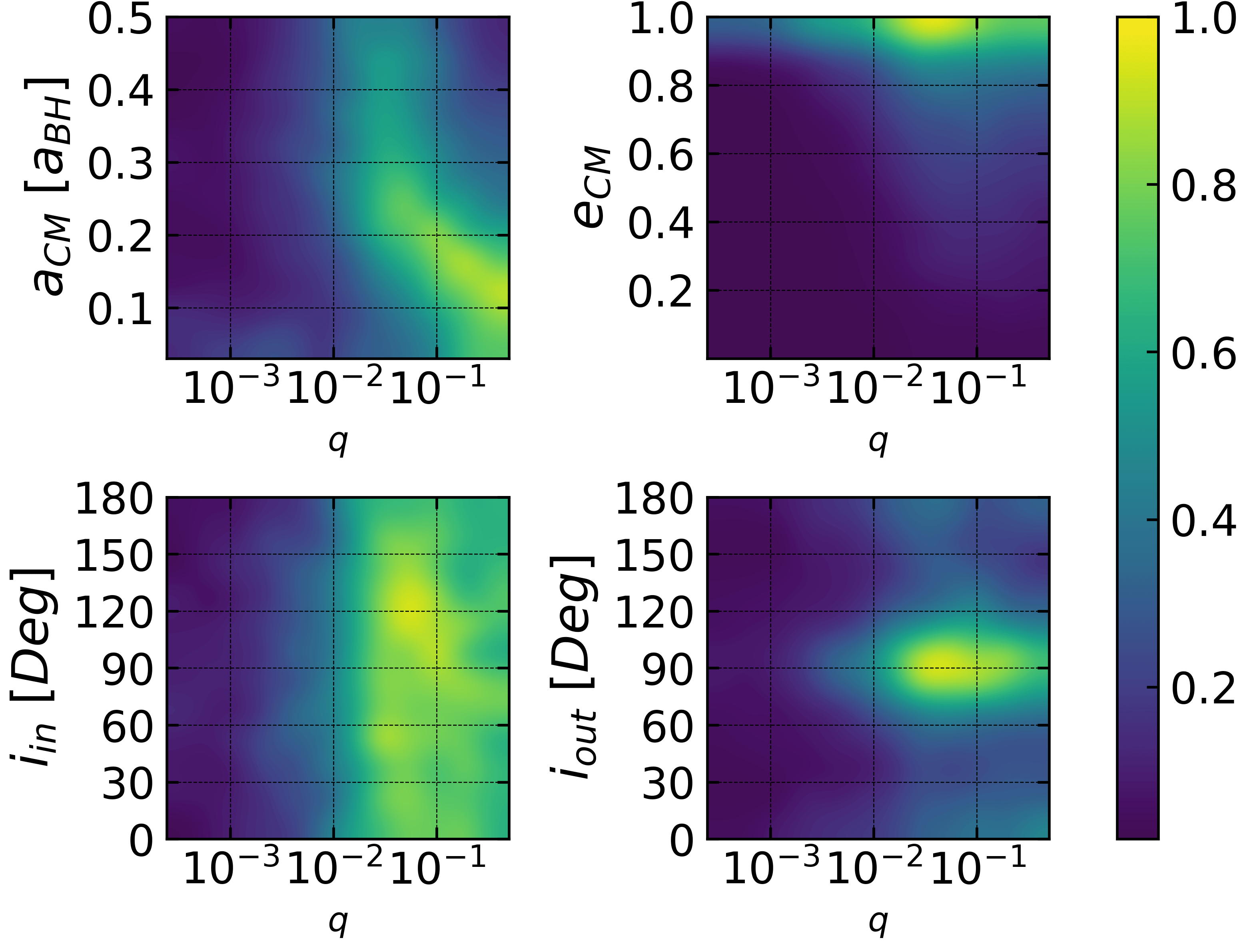
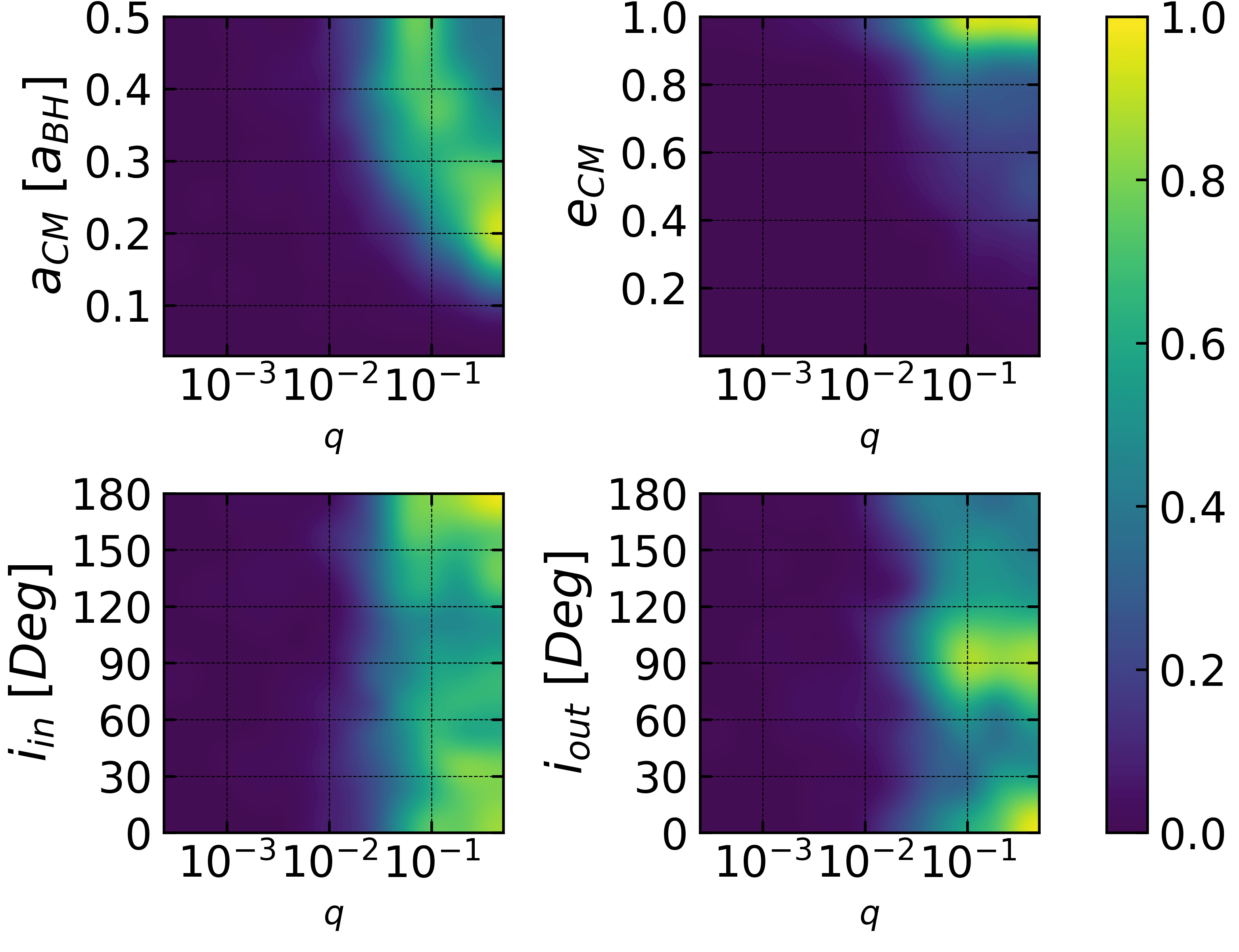
The lower panel of Fig. 11 shows the relative probabilities for the occurrence of stellar mergers. The initial parameters considered in each of the four insets are , , and . The colours quantify the relative probabilities in these parameter spaces. The first inset shows that mergers are more likely to occur at small and large . This is because, from Eq. 6 and Eq. 7, smaller and larger translates in to stronger inner LK oscillations compared to the outer LK oscillations. The third inset shows that most mergers happen when the inclination nears . This region is ideal for LK oscillations to operate effectively. The last inset confirms our earlier hypothesis, in the upper panel of Fig. 11, namely that the outer LK oscillations also contribute to mergers when even weakly concentrates at high inclination.
4.2.2 HVS rate enhancement
An interesting effect seen in our four-body system is a rapid increase in the HVS rate with increasing mass ratio. The upper panel of Fig. 12 shows the total HVS rates for different mass ratios and eccentricities . For very small mass ratios, the lines converge to the single SMBH case, and the HVS rate is nearly zero. Near the lowest mass ratios , the stability of the four-body system might be affected and breakup is possible. At larger mass ratios, the HVS rate increases significantly with increasing mass ratio . This can potentially be explained by the strong perturbation induced from the secondary SMBH on the stellar binary, which could transfer energy and angular momentum to the binary. This could even result in the collisional ejection of the binary. The bottom right panel of Fig. 7 shows a good example of this process. As is clear, a larger secondary SMBH mass along with a closer distance from the primary SMBH (i.e., larger ) result in stronger perturbations, which translates in to an elevated rate of HVS production.
The lower panel of Fig. 12 shows that HVSs are more likely to be produced at larger . This is because binaries at smaller are more likely to be consumed as TDEs due to LK oscillations. This panel also indicates that the HVS rate is independent of the outer inclination , but increases near the critical angle for LK oscillations, namely and for .
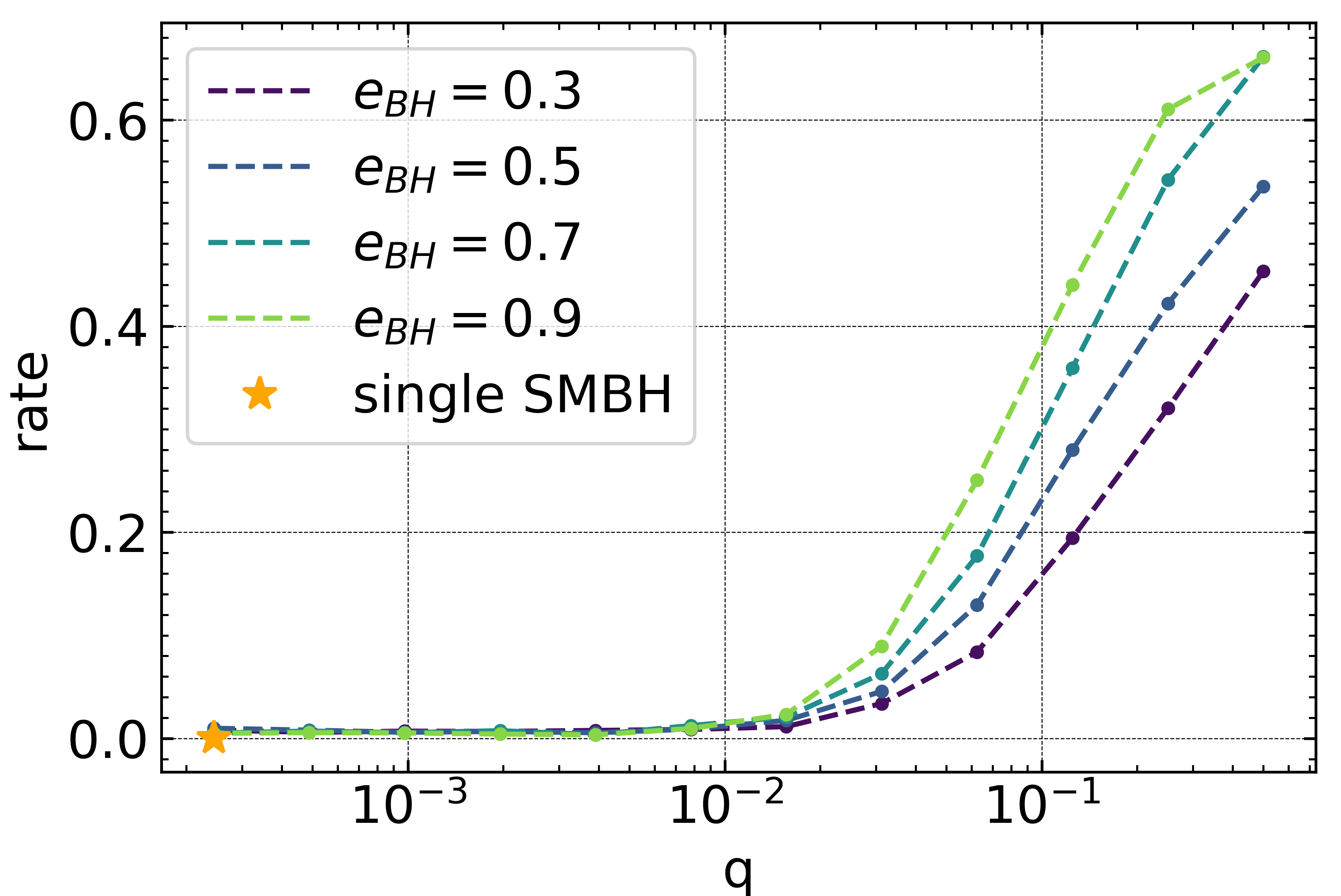
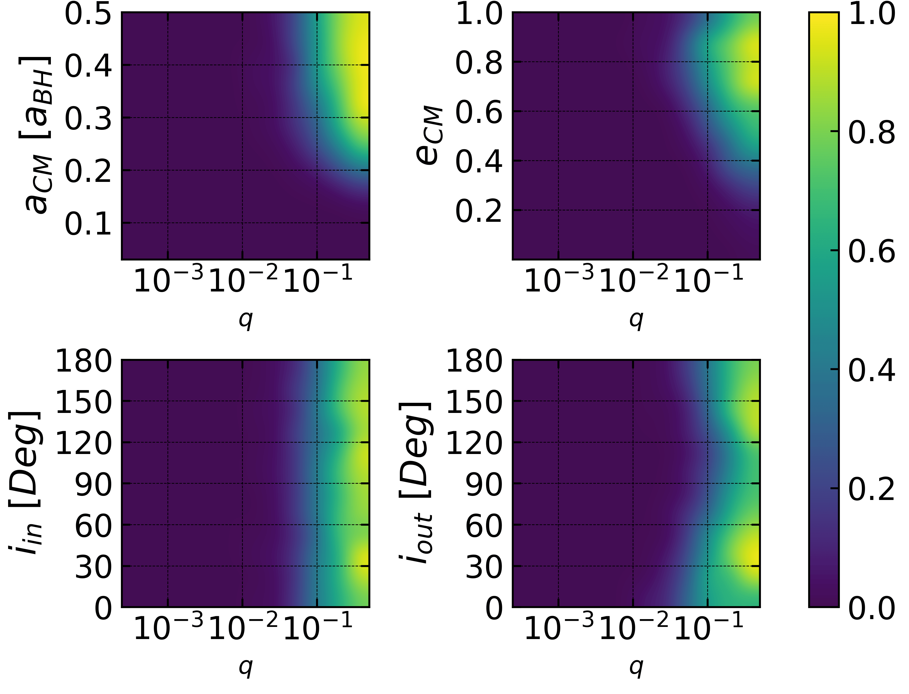
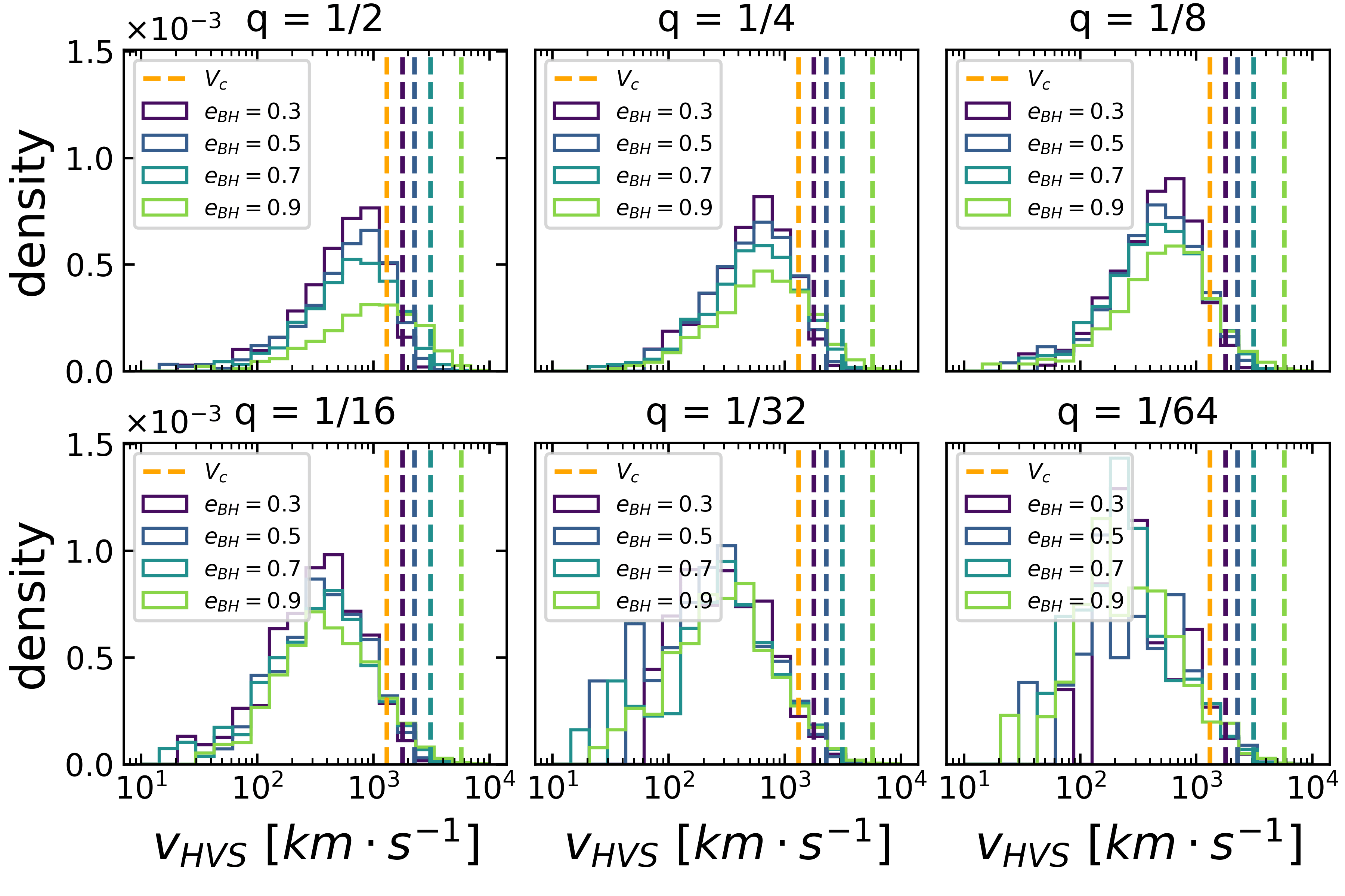
Figure 13 shows the HVS velocity distribution measured at the escape distance, or from the centre of mass of the SMBH binary. The typical escape velocity is km s-1, which fits the observations very well.
4.2.3 TDE rate enhancement
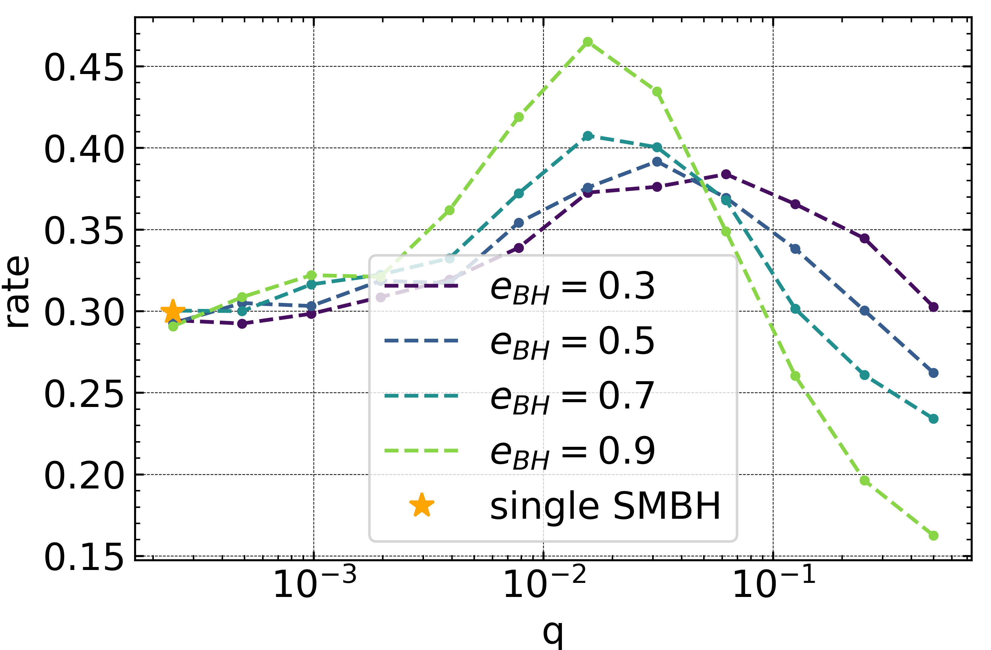
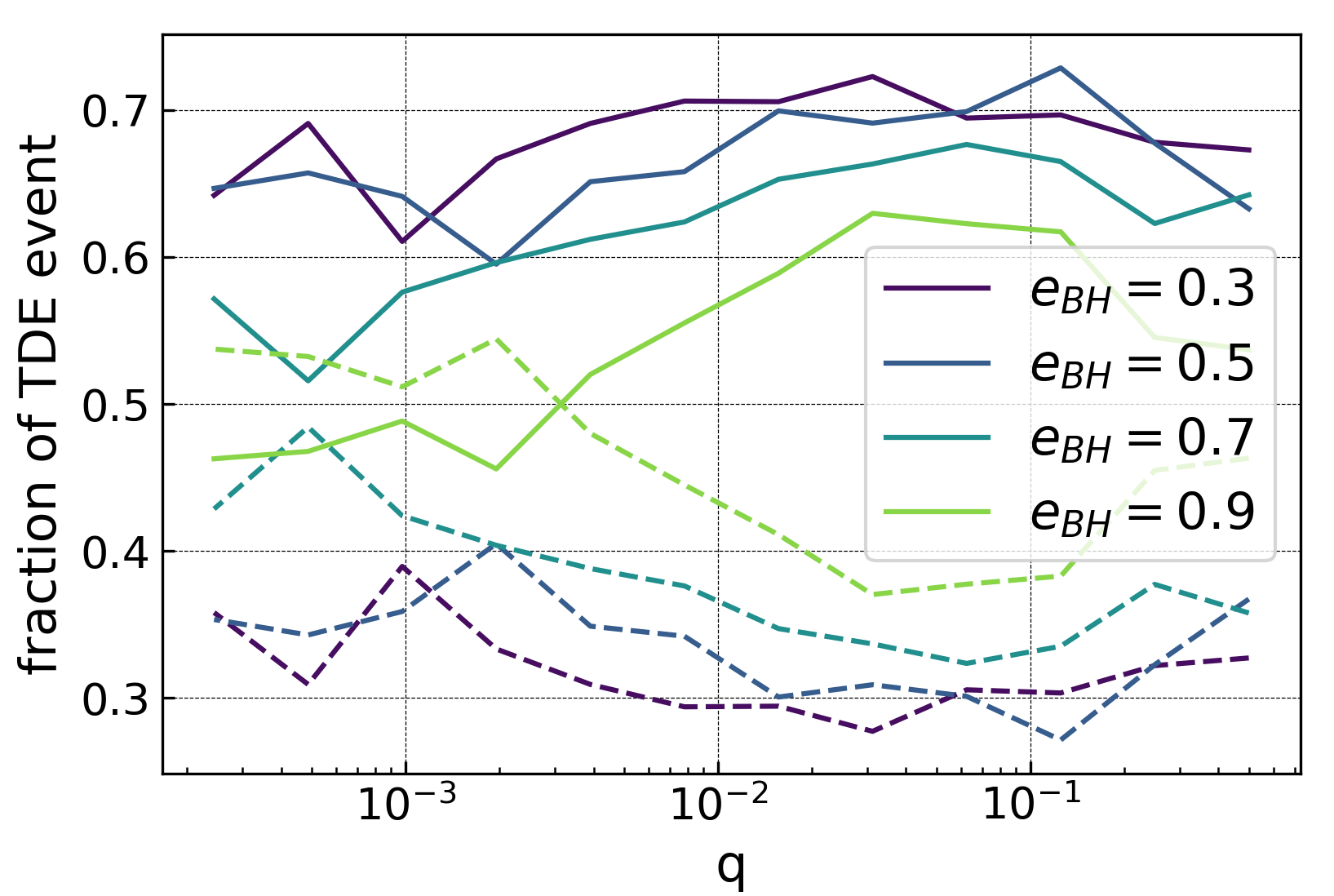
Fig.14 shows the fraction of TDEs driven by secular versus non-secular effects. We see that the relative fractions are sensitive to the eccentricity of the SMBH binary. With increasing , non-secular and chaotic effects become significant. The relative fraction has only a weak dependence on the mass ratio of the SMBH binary. However, the total TDE rate is enhanced significantly due to the presence of the secondary SMBH. LK oscillations driven by the outer orbit are the main source of the increase in the TDE rate. Equation 7 shows the outer LK oscillation time-scale. Both the mass ratio and the eccentricity increase quickly, along with a decrease in the time-scale for LK oscillations, leading to enhanced orbital excitation in the outer triple. This explains the observed increase in the TDE rate for (see the upper panel of Fig. 15). As the mass ratio increases, the stellar binary begins to feel the effects of the increasingly massive secondary SMBH . Consequently, the LK oscillations in the outer triple are gradually reduced by the presence of the secondary SMBH . This is the reason for finding that the TDE rate does not increase and can even decrease at larger mass ratios. The TDE rate for the single SMBH case at the far left end drops from to . This is due to the gap in the single TDE rate from Fig. 8.
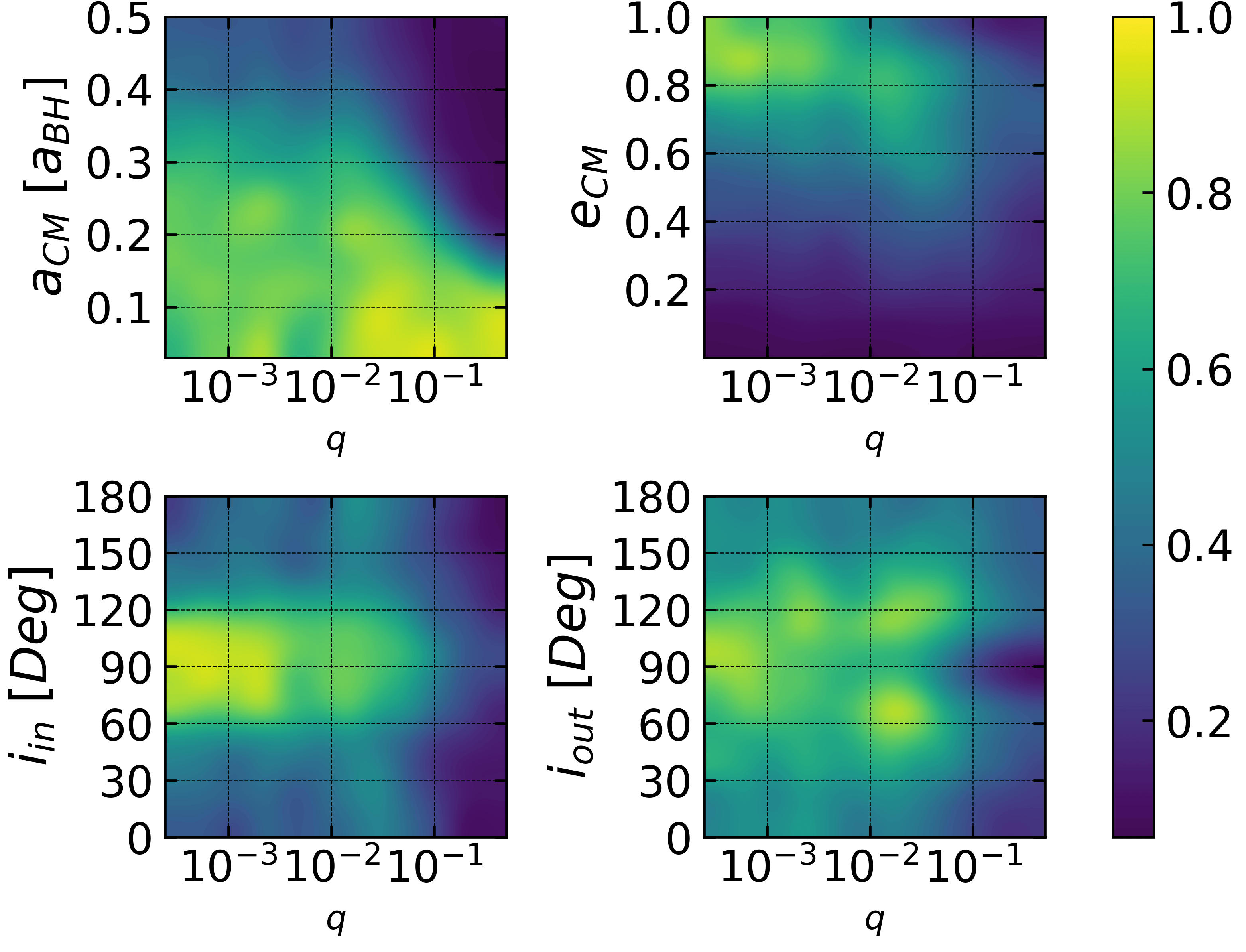
The second SMBH enhances the TDE rate significantly, from to for and from to for . The LK oscillations require that the outer triple orbit must have an outer inclination . The lower panel of Fig. 15 shows these effects mediated by LK oscillations. Most TDEs appear at high inclinations , when the outer LK oscillations dominate. This panel also clearly illustrates that the TDE rate is independent of the inner inclination .
4.2.4 HVS with TDE
A special event in this four-body system is the simultaneous occurrence of an HVS with a TDE. The stellar binary is disrupted when reaches the Hill radius . One of the stars then gets ejected as an HVS, while the other star falls into the tidal radius of one of the SMBHs (usually the primary, but see Figure 17). The binary disruption plays a fundamental role in this special event. As discussed in Section 4.2.2, in certain regions of the relevant parameter space, the secondary SMBH can transfer energy and angular momentum to the stellar binary. Subsequently, the binary can be collisionally ejected from the system. If the distance of the stellar binary to the primary SMBH remains sufficiently large, the stellar binary can remain bound and be ejected as a bound object.
Figure 16 shows the event rate for the simultaneous formation of an HVS and a TDE (i.e., HVS&TDE combination), for different eccentricities . The simulated data resemble what we would naively expect from a simple superposition of the TDE and HVS data, albeit with a few additional modifications. Although the dependence of energy and angular momentum redistribution within the four-body system on the mass ratio is not completely understood, we can still draw reliable conclusions from the lower panel of Fig. 16. In mass ratio-space, the HVS&TDE combination looks very similar to what is seen for the TDE case alone, with the exception that the former outcome extends out beyond this region to the upper right. The inner inclination concentrates at low inclination angles, such that no binary merger events occur. The outer inclination concentrates at high inclination angles, such that the decoupled star can be excited in to the tidal disruption radius.
4.3 TDE from the Secondary SMBH
Both the Schwarzschild radius and the tidal disruption radius for stars increase with increasing SMBH mass. The tidal disruption radius is given by Eq. 1, and the Schwarzschild radius is
| (17) |
Above a critical BH mass , the Schwarzschild radius becomes greater than the tidal disruption radius. Above this critical SMBH mass it should not be possible to observe any TDEs, because the SMBH will swallow the whole stars and no light will escape from within . In the limit of a primary SMBH with mass , but a secondary with mass , it is only the secondary SMBH that can cause TDE events. By incorporating the empirical relation (.e.g Kormendy & Ho, 2013; Georgiev et al., 2016), this opens up the possibility to use TDEs as detectors for secondary SMBHs/IMBHs orbiting in the nucleus of a far away galaxy. This is because, since the relation increases monotonically, it can be used to convert the critical BH mass in to a critical galaxy mass , above which no TDEs should be produced by the central SMBH. However, this assumes that the central massive BH in every galaxy is isolated. Cosmological simulations, on the other hand, suggest that both major and minor mergers between galaxy pairs occur frequently, and in the process deliver their own central SMBHs to the nuclear regions of the product of this galaxy-galaxy merger. This could predict the presence of a large population of secondary SMBHs in galaxies, in presumably stable orbits about the primary SMBH.
The presence of the secondary SMBH in orbit around the primary SMBH opens the door to observing TDEs from the secondary SMBH. But we do not know how often this should occur, if ever. To answer this question, Figure 17 shows the relative probability for a secondary-induced TDE for different mass ratios and different eccentricities . As is clear, the secondary always contributes to the total rate of TDEs, but only by a few percent at very low mass ratios. At larger mass ratios, the fraction of TDEs produced by the secondary increases steadily, converging toward 50% at . Importantly, independent of the mass ratio, the secondary always contributes a base minimum of a few percent to the total TDE rate. Extrapolating this result to even lower mass ratios suggests that even stellar-mass BHs closely orbiting a central SMBH have a non-negligible probability of causing a TDE. This begs the question: If stellar-mass BHs are in close orbits about a central massive SMBH, and each one should contribute of order a percent to the total observed TDE rate, then does the TDE rate from the SMBH become nearly equal to the TDE rate from the swarm of stellar-mass BHs? We intend to explore this interesting question in more detail in future work.
5 Summary
In this work, we have studied the fate of main sequence stellar binaries orbiting around a primary central SMBH perturbed by a remote secondary SMBH, as a function of the mass ratio of SMBH-SMBH binaries. The presence of the secondary SMBH significantly changes the evolution of these stellar binaries, and the relative rates of observable astrophysical phenomena. We have performed -body simulations of this four-body system with different SMBH-SMBH binary mass ratios, and analyzed the fate of the system. Our main conclusions can be summarized as follows.
Our simulations show that the total event (TDE, HVS, merger) rates are increased by the presence of a secondary SMBH , and continue to increase as increases (Figure 8 indicates that the fraction of uneventful simulations continuously decreases as the mass ratio increases). The presence of the secondary SMBH acts to migrate the stars toward the primary SMBH via the outer LK oscillations, where they are consumed by TDEs, HVSs and mergers. This suggests that galaxies observed to exhibit higher rates of extreme astrophysical events (i.e., TDEs, HVSs, mergers) are more likely to harbour an SMBH binary.
Merger events mainly occur due to the inner LK oscillations. Equation 6 shows the timescale for the inner LK oscillations to operate. For a given stellar mass density profile (i.e., given a distribution in ), the merger rate in a galaxy is determined by the properties of its primary SMBH. However, our simulations show that the secondary SMBH could slightly increase the merger rate in the range . In this mass ratio range, the secondary SMBH transports more stars to the inner regions near the primary SMBH. Here, the inner LK oscillations are stronger, leading to higher merger rates.
HVSs are produced from the decoupling of the stellar binary at its break up radius due to the primary SMBH. Previous work indicates that this decoupling tends to produce HVSs by ejecting one of the stars in the binary. Our simulations show that the rate for this process to operate is very low (see the rates of single HVSs in Figure 8). In this work, we have identified a more efficient way to produce HVSs, namely via strong perturbations from the secondary SMBH. These strong perturbations can even eject the stellar binary at pericenter without unbinding the binary. The rate for this process increases rapidly above mass ratios (see Figure 12). These ‘double HVSs’ should only be produced by SMBH binaries, with a rate much higher than for single HVSs.111Note that this does not account for direct interactions between a single SMBH and stellar triple systems (e.g. Perets & Subr, 2012), but the rate of these interactions should be very low (Leigh & Geller, 2013). Hence, hypervelocity binary star systems could be regarded as a smoking gun for the presence of an SMBH binary(Lu, Yu, & Lin, 2007; Sesana, Madau, & Haardt, 2009). Incidentally, one such system has possibly been identified in the Milky Way (Brown et al., 2010). Figure 13 shows the HVS velocity distribution evaluated at a distance of from the SMBH primary. The typical velocities range from to , depending on the mass ratio of the SMBH-SMBH binary. To compare the distribution of HVS velocities with observations more precisely, the Galactic potential must be taken into consideration, which will be done in a follow up paper (Wang et al. in prep.). In turn, the Galactic potential can be constrained from the observed distribution of HVSs using the upcoming data from the Gaia satellite, as discussed in (Kenyon et al., 2014; Fragione, Ginsburg, & Kocsis, 2017; Marchetti et al., 2017).
The TDE rate is quite low for the single SMBH case, relative to the SMBH-SMBH binary case. This is because the secondary SMBH acts to migrate stars to the inner region around the primary SMBH via strong outer LK oscillations. This effect could focus the stars to the centre of the galaxy, close to the primary SMBH, and in the process accelerate the rate of tidal disruption events. The secondary SMBH increases the TDE rate significantly at large mass ratios . Therefore, this opens up the possibility of using the relative rates of TDEs and HVSs to observationally constrain the occurrence of SMBH-SMBH binaries in galactic nuclei.
TDEs often occur due to disruption by the secondary SMBH, instead of the primary. This opens up the possibility of observing TDEs in massive galaxies with the most massive central SMBHs, when no TDEs should be expected. This is because, via the M- relation, the host SMBH should have a mass above the critical mass for TDEs to occur inside the Schwarzschild radius . Hence, no TDEs should be produced by the most massive SMBHs in the most massive galaxies. Thus, the observation of even a single TDE in such a massive galaxy would be the smoking gun of a secondary lower mass SMBH companion.
Our results show that the presence of a secondary SMBH changes the relative rates of TDEs and HVSs relative to the isolated SMBH case. Hence, observations of these two phenomena could help to constrain the possible presence of a central IMBH in the Galactic Centre, and/or the presence of SMBH-SMBH binaries in the nuclei of other galaxies. The dependence of the event rates in our simulations on the SMBH-SMBH binary mass ratio could potentially be used to constrain the frequency of SMBH-SMBH binaries in galactic nuclei, and even their mass ratio distribution. To this aim, a follow up paper (Wang et al. in prep.) will be devoted to a detailed comparison between simulations and all the available observational data.
Acknowledgments
YFY is supported by National Natural Science Foundation of China (Grant No. U1431228, 11725312, 11233003, and 11421303). Results in this paper were obtained using the high-performance LIred computing system at the Institute for Advanced Computational Science at Stony Brook University, which was obtained through the Empire State Development grant NYS #28451.
References
- Alexander (2005) Alexander T., 2005, PhR, 419, 65
- Anderson, Storch, & Lai (2016) Anderson K. R., Storch N. I., Lai D., 2016, MNRAS, 456, 3671
- Antonini et al. (2010) Antonini F., Faber J., Gualandris A., Merritt D., 2010, ApJ, 713, 90
- Antonini, Murray, & Mikkola (2014) Antonini F., Murray N., Mikkola S., 2014, ApJ, 781, 45
- Antonini, Murray & Mikkola (2014) Antonini F., Murray N., Mikkola S., 2014, ApJ, 781, 45
- Blaes et al. (2002) Blaes O., Lee M. H., Socrates A., 2002, ApJ, 578, 775
- Brown et al. (2010) Brown W. R., Anderson J., Gnedin O. Y., Bond H. E., Geller M. J., Kenyon S. J., Livio M. 2010, ApJL, 719, L23
- Capuzzo-Dolcetta & Fragione (2015) Capuzzo-Dolcetta R., Fragione G., 2015, MNRAS, 454, 2677
- Fragione & Capuzzo-Dolcetta (2016) Fragione G., Capuzzo-Dolcetta R., 2016, MNRAS, 458, 2596
- Fragione, Capuzzo-Dolcetta, & Kroupa (2017) Fragione G., Capuzzo-Dolcetta R., Kroupa P., 2017, MNRAS, 467, 451
- Chen et al. (2009) Chen X., Madau P., Sesana A., Liu F. K., 2009, ApJ, 697, L149
- Eggleton & Kiseleva–Eggleton (2001) Eggleton P. P. & Kiseleva–Eggleton L., 2001, ApJ, 562, 1012
- Fabrycky & Tremaine (2007) Fabrycky D. C., Tremaine S. 2007 ApJ 669 1298
- Fragione & Loeb (2017) Fragione G., Loeb A., 2017, NewA, 55, 32
- Fragione, Ginsburg, & Kocsis (2017) Fragione G., Ginsburg I., Kocsis B., 2017, arXiv, arXiv:1711.00483
- Georgiev et al. (2016) Georgiev I., Böker T., Leigh N. W. C., Lützgendorf N., Neumayer N. 2016, MNRAS, 457, 2122
- Gezari et al. (2012) Gezari S., et al., 2012, Nature, 485, 217
- Gillessen et al. (2017) Gillessen S., et al., 2017, ApJ, 837, 30
- Ginsburg & Loeb (2007) Ginsburg I., Loeb A., 2007, MNRAS, 376, 492
- Gualandris, Portegies Zwart & Sipior (2005) Gualandris A., Portegies Zwart S., Sipior M. S., 2005, MNRAS, 363, 223
- Gualandris & Merritt (2009) Gualandris A., Merritt D., 2009, ApJ, 705, 361
- Hansen, Kawaler, & Trimble (2004) Hansen C. J., Kawaler S. D., Trimble V., 2004, sipp.book
- Hills (1975) Hills J. G., 1975, Nature, 254, 295
- Hills (1988) Hills J. G., 1988, Nature, 331, 687
- Holman, Touma,& Tremaine (1997) Holman M., Touma J., Tremain S., 1997, Nature, 386, 254
- Innanen et al. (1997) Innanen K. A., Zheng J. Q., Mikkola S., Valtonen M. J., 1997, AJ, 113, 1915
- Katz & Dong (2012) Katz B., Dong S., 2012, preprint (arXiv:1211.4584)
- Kenyon et al. (2014) Kenyon S. J., Bromley B. C., Brown W. R., Geller M. J., 2014, ApJ, 793, 122
- Kormendy & Ho (2013) Kormendy J., Ho L. C., 2013, ARA&A, 51, 511
- Kozai (1962) Kozai Y., 1962, AJ, 67, 591
- Kushnir et al. (2013) Kushnir D., Katz B., Dong S., Livne E., Fernández R., 2013, ApJ, 778, L37
- Kupi, Amaro-Seoane, & Spurzem (2006) Kupi G., Amaro-Seoane P., Spurzem R., 2006, MNRAS, 371, L45
- Leigh & Geller (2013) Leigh N. W. C., Geller A. M. 2013, MNRAS, 432, 2474
- Leigh et al. (2016a) Leigh N. W. C., Antonini F., Stone N. C., Shara M. M., Merritt D. 2016, MNRAS, 463, 1605
- Leigh et al. (2016b) Leigh N. W. C., Stone N. C., Geller A. M., Shara M. M., Muddu H., Solano-Oropeza D., Thomas Y., 2016, MNRAS, 463, 3311
- Li et al. (2015) Li G., Naoz S., Kocsis B., Loeb A., 2015, MNRAS, 451, 1341
- Lidov (1962) Lidov M. L., 1962, Planet. Space Sci., 9, 719
- Lu, Yu, & Lin (2007) Lu Y., Yu Q., Lin D. N. C., 2007, ApJ, 666, L89
- Liu, Wang, & Yuan (2017) Liu B., Wang Y.-H., Yuan Y.-F., 2017, MNRAS, 466, 3376
- Liu, Lai, & Yuan (2015) Liu B., Lai D., Yuan Y.-F., 2015, PhRvD, 92, 124048
- Mandel & Levin (2015) Mandel I., Levin Y., 2015, ApJ, 805, L4
- Marchetti et al. (2017) Marchetti T., Contigiani O., Rossi E. M., Albert J. G., Brown A. G. A., Sesana A., 2017, arXiv, arXiv:1711.11397
- Martins et al. (2006) Martins F., et al. 2006, ApJ, 649, L103
- Merritt (2013) Merritt D. 2013, Dynamics and Evolution of Galactic Nuclei (Princeton: Princeton University Press)
- Miller & Hamilton (2002) Miller M. C., Hamilton D.P., 2002, ApJ, 576, 894
- Naoz et al. (2013a) Naoz S., Kocsis B., Loeb A., Yunes N., 2013a, ApJ, 773, 187
- Naoz (2016) Naoz S., 2016, ARA&A, 54, 441
- Perets (2009) Perets H. B., 2009, ApJ, 698, 1330
- Perets & Subr (2012) Perets H. B., Subr L. 2012, ApJ, 751, 133
- Phinney (1989) Phinney E. S., 1989, IAUS, 136, 543
- Prodan, Murray, & Thompson (2013) Prodan S., Murray N., Thompson T. A., 2013, preprint (arXiv:1305.2191)
- Prodan, Antonini, & Perets (2015) Prodan S., Antonini F., Perets H. B., 2015, ApJ, 799, 118
- Rees (1988) Rees M. J., 1988, Nature, 333, 523
- Ryu, Leigh, & Perna (2017) Ryu T., Leigh N. W. C., Perna R., 2017, MNRAS, 470, 3049
- Ryu, Leigh, & Perna (2017) Ryu T., Leigh N. W. C., Perna R., 2017, MNRAS, 467, 4447
- Sesana, Madau, & Haardt (2009) Sesana A., Madau P., Haardt F., 2009, MNRAS, 392, L31
- Sesana, Haardt, & Madau (2008) Sesana A., Haardt F., Madau P., 2008, ApJ, 686, 432-447
- Sesana, Haardt, & Madau (2007) Sesana A., Haardt F., Madau P., 2007, ApJ, 660, 546
- Sesana, Haardt, & Madau (2006) Sesana A., Haardt F., Madau P., 2006, ApJ, 651, 392
- Soffel (1989) Soffel M. H., 1989, S&T, 78, 382
- Storch, Anderson, & Lai (2014) Storch N. I., Anderson K. R., Lai D., 2014, Sci, 345, 1317
- Springel (2005) Springel V., 2005, MNRAS, 364, 1105
- Thompson (2011) Thompson T. A., 2011, ApJ, 741, 82
- Wen (2003) Wen L., 2003, ApJ, 598, 419
- Will (2014a) Will C. M., 2014, PhRvD, 89, 044043
- Will (2014b) Will C. M., 2014, CQGra, 31, 244001
- Wu & Murray (2003) Wu Y., Murray N., 2003, ApJ, 589, 605
- Yu & Tremaine (2003) Yu Q., Tremaine S., 2003, ApJ, 599, 1129
Appendix A
Symplectic Algorithm
The advantage of a symplectic algorithm lies in its ability to conserve the Hamiltonian structure of the system. Non-symplectic algorithms control the error to remain within a specified tolerance level, by reducing the time step length. However, if the integration time is long enough, the systematic error will accumulate non-negligibly. The rate of accumulation depends on the adopted time step length. For most gravity integrators, it is adequate to simply adjust the time step length to an acceptable value in order to ensure that the rate of error accumulation is negligible. This is because very long integration times are typically not required. However, to study systems with multi-scale dynamics (e.g., in our four-body system, the spatial scale of the SMBH binary is , but the spatial scale of the stellar binary is ), we need to make sure that we are not failing to resolve important physics, and correctly allowing for the various subtle dynamical processes characteristic of many-body systems to exert their impact on the evolution of the system. This usually requires very long integration times (e.g., the time scale for effect A to operate is much too long for effect B to have any effect, such that the shortest time-scale is what ultimately decides the integration time).
In systems with characteristic multi-scale dynamics, non-symplectic algorithms need extremely long integration times to accurately resolve the relevant physics at the minimum scale. Due to its symmetric numerical format, symplectic algorithms conserve the Hamiltonian structure for much longer integration times. Therefore, over long integration times, symplectic algorithms perform better than non-symplectic algorithms. Unfortunately, the precise symmetry applied to the numerical formatting depends on the adopted time step. This means that only algorithms that use a fixed step length are truly symplectic.
Figure 18 compares the performance of several algorithms in computing long period Keplerian orbits with the adaptive time-step method. Leapfrog and RK2 are second order algorithms. RK4, FR and PEFRL are fourth order algorithms. Leapfrog, FR and PEFRL are symplectic algorithms. RK2 and RK4 are non-symplectic algorithms.