Form Factors and Differential Branching Ratio of $B\to K\mu^{+}\mu^{-}$ in AdS/QCD

Abstract

The holographic distribution amplitudes (DAs) for the $K$ pseudoscalar meson are derived. For this aim, the light-front wave function (LFWF) of the $K$ meson is extracted within the framework of the anti de Sitter/quantum chromodynamics (AdS/QCD) correspondence. We consider a momentum-dependent (dynamical) helicity wave function that contains the dynamical spin effects. We use the LFWF to predict the radius and the electromagnetic form factor of the kaon and compare them with the experimental values. Then, the holographic twist-2 DA of $K$ meson $\phi_{{}_{K}}(\alpha,\mu)$ is investigated and compared with the result of the light-cone sum rules (LCSR). The transition form factors of the semileptonic $B\to K\ell^{+}\ell^{-}$ decays are derived from the holographic DAs of the kaon. With the help of these form factors, the differential branching ratio of the $B\to K\,\mu^{+}\mu^{-}$ on $q^{2}$ is plotted. A comparison is made between our prediction in AdS/QCD and the results obtained from two models including the LCSR and the lattice QCD as well as the experimental values.

I Introduction

The flavor changing neutral current (FCNC) transitions have received remarkable attention, both experimentally and theoretically. The decay of a $b$ quark into an $s$ quark and lepton pairs, $b\to s\ell^{+}\ell^{-}$, is a good tool to study the FCNC processes; it is also a very good way to probe the new physics effects beyond the standard model (SM).

The $B\to K\ell^{+}\ell^{-}$ decay, which occurs by the $b\to s\ell^{+}\ell^{-}$ process at the quark level, is a suitable candidate for experimental researchers who study the FCNC transition. The differential branching ratio, forward-backward, and isospin asymmetries for this transition have been measured at the BABAR, Belle, and CDF collaborations Wei ; Aaltonen ; Aaltonen1 ; Lees . Researchers in the LHCb Collaboration have reported newer results for these observable quantities Aaij1 ; Aaij2 ; Aaij3 . Recently, the updated results have been released for the differential branching fraction and the angular analysis of the $B\to K\mu^{+}\mu^{-}$ decay Bifani . On the other hand, physicists have tried to improve their results for this decay via the theoretical approaches Bouchard . Recently, a new analysis has been made to estimate the transition form factors of the $B\to K\mu^{+}\mu^{-}$ decay by the lattice QCD Bailey .

To evaluate the branching ratio and the other observable, we need to describe the intended transition according to its form factors, which are defined in terms of the distribution amplitudes (DAs). We recall that an accurate calculation of the DAs is very important since they provide a major source of uncertainty in theoretical predictions. The DAs for the $K$ pseudoscalar meson have been obtained, for the first time, from the LCSR Chernyak ; Khodjamirian1 . In recent years, a relatively new tool named the AdS/QCD correspondence has been used to obtain the DAs for the light mesons. In this approach, the wave function that describes the hadrons in the AdS space is mapped to the wave function used for the bound states in the light-front QCD. Both of them satisfy a Schrodinger-like wave function equation. The light-front DAs are derived from the holographic light-front wave function (LFWF; for instance, see Hwang12 ; Ahma1 ; Ahma3 ; Ahma4 ; ChaBro ).

So far, the isospin asymmetry of the $B\to K^{*}\mu^{+}\mu^{-}$ transition has been considered in the AdS/QCD correspondence Ahma5 . Dynamical spin effects have been taken into account of the holographic pion wave function in order to predict its mean charge radius, decay constant, the spacelike electromagnetic form factor, twist-$2$ DA, and the photon-to-pion transition form factor AhmaChish . Our goal in this paper is to extract the twist-$2$, twist-$3$ and twist-$4$ DAs of the $K$ pseudoscalar meson in the AdS/QCD method and use these holographic DAs to compute the form factors and differential branching ratio for the $B\to K\,\mu^{+}\,\mu^{-}$ transition.

Our paper is organized as follows: In Sec. II, the light-front DAs and the holographic LFWF for the $K$ pseudoscalar meson are calculated. In this section, the connection between the holographic LFWF and DAs of the $K$ meson is presented. Using the holographic DAs, the transition form factors can be investigated. In Sec. III, we use the holographic LFWF to consider the radius and the electromagnetic (EM) form factor of the $K$ meson and compare them with the experimental values. We also analyze the holographic twist-2 DA of $K$ meson $\phi_{{}_{K}}(\alpha,\mu)$ and transition form factors of the FCNC $B\to K$ transitions. Then, the differential branching ratio of $B\to K\mu^{+}\mu^{-}$ decay on $q^{2}$ is plotted. Our prediction is compared with those made by the lattice QCD and light-cone sum rule (LCSR) approaches, as well as the experimental values.

II THE HOLOGRAPHIC DISTRIBUTION AMPLITUDES FOR THE K MESON

The holographic DAs for the $K$ pseudoscalar meson are derived in this section. For this aim, we plan to obtain a connection between the DAs and the holographic LFWF of the $K$ meson. Using the definition of the DAs for the $K$ meson introduced by the meson-to-vacuum matrix elements Khodjamirian1 ; Chernyak ; Braun ; Belyaev1 , and choosing $p^{\mu}=(p^{+},\frac{m^{2}_{K}}{p^{+}},\textbf{0}_{\perp})$ for the four-momentum of the $K$ meson, the following matrix elements can be written in the light-front coordinate, $x^{\mu}=(x^{+},x^{-},\textbf{x}_{\perp})$, at equal light-front time, $x^{+}=0$, as

$$\langle 0|\bar{u}(0)\gamma^{\alpha}\gamma^{5}s(x^{{}_{-}})|K(p)\rangle = i\,f_{{}_{K}}p^{\alpha}\int_{0}^{1}du\,e^{-iup^{+}x^{-}}\phi_{{}_{K}}(u,\mu)\,,$$ (1)

$$\langle 0|\bar{u}(0)\gamma^{5}s(x^{{}_{-}})|K(p)\rangle = -i\,\frac{f_{{}_{K}}m^{2}_{{}_{K}}}{m_{u}+m_{s}}\int_{0}^{1}du\,e^{-iup^{+}x^{-}}\phi_{\rho}(u,\mu)\,,$$ (2)

$$\langle 0|\bar{u}(0)\sigma^{\alpha\beta}(1+\gamma^{5})s(x^{{}_{-}})|K(p)\rangle = \frac{i}{6}\,\frac{f_{{}_{K}}m^{2}_{{}_{K}}}{(m_{u}+m_{s})}\,p^{[{\alpha}}x^{\beta]}\int_{0}^{1}du\,e^{-iup^{+}x^{-}}\phi_{\sigma}(u,\mu)\,,$$ (3)

$$\langle 0|\bar{u}(0)\gamma^{\alpha}s(x^{{}_{-}})|K(p)\rangle = i\,f_{{}_{K}}{(x^{-})}^{2}p^{\alpha}\int_{0}^{1}du\,e^{-iup^{+}x^{-}}g_{1}(u,\mu)-f_{{}_{K}}(x^{\alpha}-\frac{x^{-}}{p^{+}}p^{\alpha})$$ (4)

$$\times \int_{0}^{1}du\,e^{-iup^{+}x^{-}}g_{2}(u,\mu)\,,$$

where $\mu$ is the renormalization scale and $f_{{}_{K}}$ is the decay constant of the $K$ pseudoscalar meson. In these relations, $\phi_{{}_{K}}$ is twist-2, $\phi_{\rho}$ and $\phi_{\sigma}$ are twist-3, and $g_{1}$ and $g_{2}$ are twist-4 DAs for the $K$ meson. To isolate $\phi_{{}_{K}}$ and $\phi_{\rho}$, we take $\alpha=+$ and apply the Fourier transform of Eqs. (1) and (2) with respect to $x^{-}$. It yields

$$\phi_{{}_{K}}(\alpha,\mu) = -\frac{i}{f_{K}}\int dx^{-}\,e^{i\alpha p^{+}x^{-}}\langle 0|\bar{u}(0)\gamma^{\alpha}\gamma^{5}s(x^{{}_{-}})|K(p)\rangle,$$ (5)

$$\phi_{\rho}(\alpha,\mu) = i\frac{(m_{u}+m_{s})}{f_{{}_{K}}m^{2}_{{}_{K}}}p^{+}\int dx^{-}\,e^{i\alpha p^{+}x^{-}}\langle 0|\bar{u}(0)\gamma^{5}s(x^{{}_{-}})|K(p)\rangle.$$ (6)

Choosing $\sigma^{+-}$ in Eq. (3), and using integration by parts with the boundary condition $\phi(u)|^{1}_{0}=0$, as well as performing the Fourier transform with respect to $x^{{}_{-}}$, the derivative of the twist-3 $\phi_{\sigma}(\alpha,\mu)$ is obtained as

$$\frac{\partial\phi_{\sigma}(\alpha,\mu)}{\partial\alpha} = \frac{6(m_{u}+m_{s})}{f_{{}_{K}}m^{2}_{{}_{K}}}p^{+}\int dx^{-}e^{i\alpha p^{+}x^{-}}\langle 0|\bar{u}(0)\sigma^{+-}(1+\gamma^{5})s(x^{-})|K(p)\rangle.$$ (7)

Taking $\alpha=+$ (and afterwards $\alpha=-$) in Eq. (4), and then using integration by part, the following relations are derived:

$$\langle 0|\bar{u}(0)\gamma^{+}s(x^{-})|K(p)\rangle = \frac{if_{{}_{K}}}{p^{+}}\Bigg{[}\int_{0}^{1}du\,e^{-iup^{+}x^{-}}\,\frac{\partial^{2}g_{1}(u,\mu)}{\partial u^{2}}-\int_{0}^{1}du\,e^{-iup^{+}x^{-}}\,\frac{\partial g_{2}(u,\mu)}{\partial u}\Bigg{]},$$ (8)

$$\langle 0|\bar{u}(0)\gamma^{-}s(x^{-})|K(p)\rangle = \frac{if_{{}_{K}}}{p^{+}}\Bigg{[}\frac{m_{K}^{2}}{(p^{+})^{2}}\int_{0}^{1}du\,e^{-iup^{+}x^{-}}\,\frac{\partial^{2}g_{1}(u,\mu)}{\partial u^{2}}\,-\left(1-\frac{m_{K}^{2}}{(p^{+})^{2}}\right)$$ (9)

$$\times \int_{0}^{1}du\,e^{-iup^{+}x^{-}}\,\frac{\partial g_{2}(u,\mu)}{\partial u}\Bigg{]}.\,$$

Solving Eqs. (8) and (9) in terms of $\frac{\partial^{2}g_{1}(u,\mu)}{\partial u^{2}}$ and $\frac{\partial g_{2}(u,\mu)}{\partial u}$, as well as performing the Fourier transform with respect to $x^{-}$, we obtain

$$\frac{\partial g_{2}(\alpha,\mu)}{\partial\alpha} = \frac{i}{f_{K}[2m_{K}^{2}-(p^{+})^{2}]}\int dx^{-}e^{i\alpha p^{+}x^{-}}$$ (10)

$$\times \left[\frac{m_{K}^{2}}{(p^{+})^{2}}\langle 0|\bar{u}(0)\gamma^{+}s(x^{-})|K(p)\rangle-\langle 0|\bar{u}(0)\gamma^{-}s(x^{-})|K(p)\rangle\right],$$

$$\frac{\partial^{2}g_{1}(\alpha,\mu)}{\partial\alpha^{2}} = \frac{i}{f_{K}[2m_{K}^{2}-(p^{+})^{2}]}\int dx^{-}e^{i\alpha p^{+}x^{-}}$$ (11)

$$\times \left[(\frac{m_{K}^{2}}{(p^{+})^{2}}-1)\langle 0|\bar{u}(0)\gamma^{+}s(x^{-})|K(p)\rangle-\langle 0|\bar{u}(0)\gamma^{-}s(x^{-})|K(p)\rangle\right].$$

In order to evaluate the holographic DAs for the $K$ meson, the hadronic matrix elements should be determined in Eqs. (5) -(7) and (10)-(11). For this purpose, the Fock expansion of noninteracting two-particle states is used for a hadronic eigenstate $|P\rangle$ as R1

$$|P(p)\rangle=\sqrt{4\pi N_{c}}\sum_{h,\bar{h}}\int\frac{dk^{+}d^{2}{\bf{k}_{\bot}}}{16\pi^{3}\sqrt{k^{+}(p^{+}-k^{+})}}\Psi^{P}_{h,\bar{h}}(\frac{k^{+}}{p^{+}},{\bf{k}_{\bot}})|k^{+},\textbf{k}_{\bot},h;\,p^{+}-k^{+},-\textbf{k}_{\bot},\bar{h}\rangle,$$ (12)

in which $\Psi^{P}_{h,\bar{h}}(\alpha,{\bf{k}_{\bot}})$ is the LFWF of the pseudoscalar meson, and $h$ and $\bar{h}$ are the helicities of the quark and anti-quark, respectively. By utilizing the expansion of Dirac fields (quark and antiquark) in terms of particle creation and annihilation operators, and also the equal light-front time anticommination relations for these operators, the matrix element $\langle 0|\bar{u}(0)\,\Gamma\,s(x^{-})|P(p)\rangle$ is obtained as

$$\langle 0|\bar{u}(0)\,\Gamma\,s(x^{-})|P(p)\rangle = \sqrt{4\pi N_{c}}\sum_{h,\bar{h}}\int\frac{dk^{+}d^{2}{\bf{k}_{\bot}}\,\Theta(|\mathbf{k}_{\bot}|<\mu)}{16\,\pi^{3}\sqrt{k^{+}(p^{+}-k^{+})}}\Psi^{P}_{h,\bar{h}}(\alpha,{\bf{k}_{\bot}})$$ (13)

$$\times\bar{v}_{\bar{h}}(p^{+}-k^{+},-{\bf{k}_{\bot}})\,\Gamma\,u_{h}(k^{+},{\bf{k}_{\bot}})e^{-ik^{+}x^{-}}\,,$$

in which $u_{h}$ and $v_{h}$ are light-front helicity spinors for the quark and antiquark, respectively. The renormalization scale $\mu$ is used as the ultraviolet cutoff on transverse momenta Kogut ; Diehl . In our work, $\Gamma$ can be $\sigma^{+-}(1+\gamma^{5})$, $\gamma^{+}$, or $\gamma^{-}$. By integrating with respect to $k^{+}$ and applying the Fourier transform to the left and right- hand sides of Eq. (13), the following result is obtained:

$$\int dx^{-}e^{i\alpha p^{+}x^{-}}\langle 0|\bar{u}(0)\,\Gamma\,s(x^{-})|P(p)\rangle = \frac{\sqrt{4\pi N_{c}}}{p^{+}}\sum_{h,\bar{h}}\int^{|\mathbf{k}_{\bot}|<\mu}\frac{d^{2}\mathbf{k}_{\bot}}{(2\pi)^{3}}\Psi^{P}_{h,\bar{h}}(\alpha,\mathbf{k}_{\bot})$$

$$\times\left\{\frac{\bar{v}_{\bar{h}}(\bar{\alpha}\,p^{+},-\mathbf{k}_{\bot})}{\sqrt{\bar{\alpha}}}\,\Gamma\,\frac{u_{h}(\alpha\,p^{+},\mathbf{k}_{\bot})}{\sqrt{\alpha}}\right\}\,,$$

where $\alpha=\frac{k^{+}}{p^{+}}$, and $\bar{\alpha}=1-\alpha$. In the $\mathbf{k}$ space, the holographic LFWF is given as R1

$$\Psi^{P}_{h,\bar{h}}(\alpha,\mathbf{k}_{\bot})=\frac{1}{\sqrt{4\pi}}S^{P}_{h,\bar{h}}(\alpha,\mathbf{k}_{\bot})\phi(\alpha,\mathbf{k}_{\bot}).$$ (15)

The structure of $S^{P}_{h,\bar{h}}(\alpha,\mathbf{k}_{\bot})$ for the pseudoscalar mesons that includes the helicity-dependent wave function is as follows:

$$S_{h,\bar{h}}^{P}(\alpha,\mathbf{k}_{\bot})=\frac{\bar{u}_{h}(\alpha\,p^{+},-\mathbf{k}_{\bot})}{\sqrt{\alpha}}\,\left[(A\not\!p+Bm_{{}_{K}})\gamma^{5}\right]\frac{v_{\bar{h}}(\bar{\alpha}\,p^{+},\mathbf{k}_{\bot})}{\sqrt{\bar{\alpha}}}\,,$$ (16)

where $A$ and $B$ are arbitrary constants. If $B\neq 0$, the dynamical spin effects are allowed. For considering the dynamical spin effects, $A$ and $B$ are usually taken in two cases: $(A=0;B=1)$ and $(A=1;B=1)$ AhmaChish ; Heinzl ; Choi ; Trawiski ; ChaBro .

Using the light-front spinors presented in Ref. Brodsky6 , $S_{h,\bar{h}}^{P}$ is evaluated for the $K$ meson as

$$i\,S_{h,\bar{h}}^{K}(\alpha,\mathbf{k}_{\bot}) = \mp\frac{A}{\alpha\bar{\alpha}}\Bigg{\{}\left[\alpha\bar{\alpha}\,m_{{}_{K}}^{2}+m_{u}m_{s}+{k}^{2}\right]\delta_{h\pm,\bar{h}\mp}\pm{k}\left[m_{u}e^{-i\theta_{k}}\delta_{h+,\bar{h}+}+m_{s}e^{i\theta_{k}}\delta_{h-,\bar{h}-}\right]\Bigg{\}}$$ (17)

$$\mp \frac{B\,m_{{}_{K}}}{\alpha\bar{\alpha}}\left[\alpha\,m_{s}+\bar{\alpha}\,m_{u}\mp{k}e^{\mp i\theta_{k}}\right]\delta_{h\pm,\bar{h}\mp}\,,$$

where $ke^{\pm i\theta_{k}}$ is the complex form of the transverse momentum $\mathbf{k}_{\bot}$; in addition, $h+$ and $h-$ are used for positive and negative helicity, respectively.

The light-front spinors are also utilized to obtain the matrix elements in the right-hand side of Eq. (II). The final results can be written as

$$\frac{\bar{v}_{\bar{h}}}{\sqrt{\bar{\alpha}}}\gamma^{+}\frac{u_{h}}{\sqrt{\alpha}} = 2p^{+}\delta_{h\pm,\bar{h}\mp}\,,$$

$$\frac{\bar{v}_{\bar{h}}}{\sqrt{\bar{\alpha}}}\gamma^{-}\frac{u_{h}}{\sqrt{\alpha}} = 2p^{+}\delta_{h\pm,\bar{h}\mp}\,,$$

$$\frac{\bar{v}_{\bar{h}}}{\sqrt{\bar{\alpha}}}\gamma^{+}\gamma^{5}\frac{u_{h}}{\sqrt{\alpha}} = \pm\,2p^{+}\delta_{h\pm,\bar{h}\mp}\,,$$

$$\frac{\bar{v}_{\bar{h}}}{\sqrt{\bar{\alpha}}}\gamma^{5}\frac{u_{h}}{\sqrt{\alpha}} = \frac{1}{\alpha\,\bar{\alpha}}\left\{ke^{\pm i\theta_{k}}\delta_{h\pm,\bar{h}\pm}\mp\left(\alpha\,m_{s}+\bar{\alpha}\,m_{u}\right)\delta_{h\pm,\bar{h}\mp}\right\},$$

$$\frac{\bar{v}_{\bar{h}}}{\sqrt{\bar{\alpha}}}\sigma^{+-}(1+\gamma^{5})\frac{u_{h}}{\sqrt{\alpha}} = \frac{4\,i}{\alpha\,\bar{\alpha}}\left\{\mp ke^{\pm i\theta_{k}}\,(1-2\,\alpha)\delta_{h\pm,\bar{h}\pm}+\alpha\,m_{{u}}\,\delta_{h+,\bar{h}-}+\bar{\alpha}\,m_{s}\,\delta_{h-,\bar{h}+}\right\}.$$ (18)

Inserting Eqs. (17)-(18) in Eq. (II), the hadronic matrix elements in Eqs. (5)-(7) and (10)-(11) are determined. Therefore, the holographic DAs can be calculated for the $K$ meson in terms of $\phi(\alpha,\mathbf{k}_{\bot})$ in the k space. Applying the Fourier transform to $r$ space and using relations such as $\int_{0}^{2\pi}e^{-ikrcos\theta}d\theta=2\pi J_{0}(kr)$, and $\int_{0}^{\mu}k\,J_{0}(kr)\,d(kr)={\mu}/{r}\,J_{1}(\mu r)$, where $J_{0}$ and $J_{1}$ are Bessel functions, the following expressions are obtained for the holographic DAs in the $r$ space:

$$\phi_{{}_{K}}(\alpha,\mu) = \frac{\beta_{1}}{\alpha\bar{\alpha}}\int{dr}\,\mu J_{1}(\mu r)\left\{2A\left(\alpha\bar{\alpha}m_{{}_{K}}^{2}+m_{u}m_{s}-\nabla^{2}\right)+Bm_{{}_{K}}\left(\bar{\alpha}\,m_{u}+\alpha\,m_{s}\right)\right\}\phi(\alpha,r),$$

$$\phi_{\rho}(\alpha,\mu) = -\frac{(m_{s}+m_{u})\beta_{1}}{\alpha^{2}\bar{\alpha}^{2}\,m_{{}_{K}}^{2}}\int{dr}\,\mu J_{1}(\mu r)\Big{\{}A\left[(\alpha\,m_{u}+\bar{\alpha}\,m_{s})\left(\alpha\bar{\alpha}m_{{}_{K}}^{2}+m_{u}m_{s}-\nabla^{2}\right)\right.$$

$$- \left.(m_{u}+m_{s})\nabla^{2}\right]-Bm_{{}_{K}}\left[\left(\alpha m_{s}+\bar{\alpha}m_{u}\right)^{2}-\nabla^{2}\right]\Big{\}}\,\phi(\alpha,r),$$

$$\frac{\partial\phi_{\sigma}(\alpha,\mu)}{\partial\alpha} = -\frac{24(m_{u}+m_{s})\beta_{1}}{\alpha^{2}\bar{\alpha}^{2}\,m_{{}_{K}}^{2}}\int{dr}\,\mu J_{1}(\mu r)\Big{\{}A\left[(\alpha\,m_{u}-\bar{\alpha}\,m_{s})\left(\alpha\bar{\alpha}m_{{}_{K}}^{2}+m_{u}m_{s}-\nabla^{2}\right)\right.$$

$$- \left.(2\alpha-1)(m_{u}-m_{s})\nabla^{2}\right]+Bm_{{}_{K}}\left[\alpha^{2}m^{2}_{u}-\bar{\alpha}^{2}m^{2}_{s}-(2\alpha-1)\nabla^{2}\right]\Big{\}}\,\phi(\alpha,r),$$

$$\frac{\partial g_{2}(\alpha,\mu)}{\partial\alpha} = \frac{\beta_{1}\beta_{2}}{\beta_{3}\,\alpha\bar{\alpha}m_{{}_{K}}}\int{dr}\,\mu J_{1}(\mu r)\,B\left[\alpha\,m_{\bar{u}}+\bar{\alpha}\,m_{s}\right]\phi(\alpha,r),$$

$$\frac{\partial^{2}g_{1}(\alpha,\mu)}{\partial\alpha^{2}} = \frac{\beta_{1}(\beta_{2}-1)}{\beta_{3}\,\alpha\bar{\alpha}m_{{}_{K}}}\int{dr}\,\mu J_{1}(\mu r)\,B\left[\alpha\,m_{u}+\bar{\alpha}\,m_{s})\right]\phi(\alpha,r),$$ (19)

where $\sqrt{N_{c}}/(\pi\,f_{K})=\beta_{1}$, $\left[1-{m_{{}_{K}}^{2}}/{{(p^{+})}^{2}}\right]=\beta_{2}$ and $\left[2-{{(p^{+})}^{2}}/{m_{{}_{K}}^{2}}\right]=\beta_{3}$.

To specify $\phi(\alpha,r)$, which includes dynamical properties of $K$ in the LFWF, we are going to use the AdS/QCD. Based on a first semiclassical approximation to the light-front QCD, with massless quarks, function $\phi$ can be factorized as GFdeSJBr

$$\phi(\zeta,\alpha,\theta)=\mathcal{N}\frac{\psi(\zeta)}{\sqrt{2\pi\zeta}}\,f(\alpha)\,e^{iL\theta},$$ (20)

where $\mathcal{N}$ is a normalization constant. In this relation, $L$ is the orbital angular momentum quantum number and variable $\zeta=\sqrt{\alpha(1-\alpha)}\,r$, where $r$ is the transverse distance between the quark and antiquark forming the meson. Function $\psi(\zeta)$ satisfies the so-called holographic light-front Schrodinger-like equation as

$$\left(-\frac{d^{2}}{d\zeta^{2}}-\frac{1-4L^{2}}{4\zeta^{2}}+U(\zeta)\right)\psi(\zeta)=M^{2}\psi(\zeta),$$ (21)

where $M$ is the hadron bound-state mass and $U(\zeta)$ is the effective potential. It should be noted that all the interaction terms and the effects of higher Fock states on the valence ($N=2$ for mesons) state are hidden in the confinement potential.

According to the AdS/QCD, the holographic light-front Schrodinger equation is mapped onto the wave equation for strings propagating in the AdS space if $\zeta$ is identified with the fifth dimension in AdS space. To illustrate this issue, the invariant action (up to bilinear terms) is written for a scalar field in the AdS₅ space as

$$S=\frac{1}{2}\int\!d^{4}x\,dz\,\sqrt{g}\,e^{\varphi(z)}\left(g^{MN}\partial_{M}\Phi\partial_{N}\Phi-\mu^{2}\Phi^{2}\right),$$ (22)

where $g={(\frac{R}{z})}^{10}$ is the modulus of the determinant of the metric tensor $g_{MN}$. Moreover, $\Phi(x^{\mu},z)$ is a scalar field. Mass $\mu$ in Eq. (22) is not a physical observable. In this action, the dilaton background $\varphi(z)$ is only a function of the holographic variable $z$ that vanishes if $z\to\infty$. Variation of Eq. (22) and making the ansatz $\Phi(x^{\mu},z)=e^{-iP\cdot x}\Theta(z)$, which describe a free hadronic state with four-momentum $P$ in holographic QCD, the eigenvalue equation is obtained as

$$\left[-\frac{z^{3}}{e^{\varphi(z)}}\partial_{z}\left(\frac{e^{\varphi}(z)}{z^{3}}\partial_{z}\right)+\left(\frac{\mu R}{z}\right)^{2}\right]\Theta(z)={M}^{2}\Theta(z),$$ (23)

where $P_{\mu}P^{\mu}=M^{2}$ is the invariant mass. Factoring out the scale $(1/z)^{-\frac{3}{2}}$ and dilaton factors from the AdS field as $\Theta=({\frac{R}{z}})^{-\frac{3}{2}}e^{-\varphi(z)/2}\psi(z)$, and using a substitution as $z\to\zeta$, the light-front Schrodinger equation [Eq. (21)] is fined with the effective potential $U(\zeta)=\frac{1}{2}\varphi^{\prime\prime}(\zeta)+\frac{1}{4}\varphi^{\prime}(\zeta)^{2}-\frac{1}{\zeta}\varphi^{\prime}(\zeta)$, and the AdS mass $(\mu R)^{2}=L^{2}-1$. In this correspondence, $\varphi(\zeta)$ and $(\mu R)^{2}$ are related to the effective potential and the internal orbital angular momentum $L$, respectively.

Choosing $\varphi(\zeta)=\kappa^{2}\zeta^{2}$ in the soft-wall model Karch leads to $U(\zeta)=\kappa^{4}\zeta^{2}-2\kappa^{2}$. It should be noted that the harmonic form of this potential is unique that is the most remarkable feature of the light-front holographic QCD Teramond . Solving Eq. (23) with this potential and comparing the equation with the quantum mechanical oscillator in the polar coordinates, the results are obtained for eigenfunctions [$\psi_{n,L}(\zeta)$] and eigenvalues [$M^{2}(n,L,S)$].

Therefore, $\phi(r,\alpha)$ for the $K$ meson with massless quarks, and $n=0$, $L=0$, is obtained as

$$\phi(\alpha,\zeta)=\mathcal{N}\frac{\kappa}{\sqrt{\pi}}\sqrt{\alpha\bar{\alpha}}\exp\left(-\frac{\kappa^{2}\zeta^{2}}{2}\right),$$ (24)

where $\kappa$ is the AdS/QCD scale. It should be noted that the condition $\int_{0}^{1}d\alpha\frac{f(\alpha)^{2}}{\alpha\,\bar{\alpha}}=1$ is used to determine the function $f(\alpha)$ in Eq. (20) GFdeSJBr . To include the mass of quarks in Eq. (24), first, a Fourier transform is applied to k space as $\widetilde{\phi}(\alpha,\textbf{k}_{\bot})=\int\,d^{2}\textbf{r}\,e^{-ikr\cos\theta_{k}}\,\phi(\alpha,\zeta)$; it yields

$${\widetilde{\phi}}(\alpha,\textbf{k}_{\bot})=\mathcal{N}\,\frac{2}{\sqrt{\alpha\bar{\alpha}\,}}\,\frac{\sqrt{\pi}}{\kappa}\exp\left(-\frac{k^{2}}{2\alpha\bar{\alpha}\,\kappa^{2}}\right);$$ (25)

then, this substitution is used BroTera5 ,

$$\frac{k^{2}}{\alpha\bar{\alpha}}\to\frac{k^{2}}{\alpha\bar{\alpha}}+\frac{m_{u}^{2}}{\alpha}+\frac{m^{2}_{s}}{\bar{\alpha}}.$$ (26)

After substituting this into the wave function and Fourier transforming back to the transverse position space, the final form of the AdS/QCD wave function is obtained as

$$\phi(\zeta,\alpha)=\mathcal{N}\,\frac{\kappa}{\sqrt{\pi}}\,\sqrt{\alpha\,\bar{\alpha}}\exp\left(-\frac{\kappa^{2}\zeta^{2}}{2}\right)\exp\left\{-\left[\frac{\bar{\alpha}\,m_{u}^{2}-\alpha\,m^{2}_{s})}{2\alpha\bar{\alpha}\,\kappa^{2}}\right]\right\}.$$ (27)

In position space, $\mathcal{N}$ can be fixed by this normalization condition R1 ,

$$\int d^{2}{\mathbf{r}}\,d\alpha\Bigg{[}\sum_{h,\bar{h}}|\Psi^{K}_{h,\bar{h}}(r,\alpha)|^{2}\Bigg{]}=1.$$ (28)

III Numerical analysis

In this section, we present our numerical analysis for the light-front holographic DAs of the $K$ meson, the $B\to K\ell^{+}\ell^{-}$ transition form factors, as well as the differential branching ratio of the $B\to K\mu^{+}\mu^{-}$ transition on $q^{2}$.

According to the light-front holographic prediction, the mass squared of mesons composed of light quarks is given as $M^{2}(n,L,S)=4\,\kappa^{2}\,(n+L+\frac{S}{2})$, where the quantum numbers $L$ and $n$ describe the orbital angular momentum and excitations of the meson spectrum, respectively. By fitting this mass relation to the experimentally measured Regge slopes, the AdS/QCD scale $\kappa$ is reported to be $590~{}\rm{MeV}$ for pseudoscalar mesons Teramond . In this paper, we choose $\kappa=590~{}\rm{MeV}$ in our analysis. In addition, we consider two sets for $A$ and $B$ as set I $(A=1;B=1)$ and set II $(A=0;B=1)$ that allow for considering the dynamical spin effects.

Using the experimental values of the decay constants, $f_{\pi}$ and $f_{K}$, and choosing the value of $\kappa$, we can obtain the mass of the light quarks related to our analysis; they are in fact the effective quark masses used in the holographic LFWFs Teramond . The decay constant for a pseudoscalar meson, which contains $q$ and $q^{\prime}$ quarks, can be defined as

$$\langle 0|\bar{q}(0)\gamma^{\alpha}\,\gamma^{5}\,q^{\prime}(0)|S(p)\rangle=if_{S}\,p^{\alpha}.$$ (29)

After expanding the left-hand side of Eq. (29) in the procedure described in the previous section, the decay constant formula for the pion and kaon in the AdS/QCD correspondence is calculated as

$$f_{S} = \frac{\sqrt{N_{c}}}{\pi}\int_{0}^{1}d\alpha\,\left[B\left(\bar{\alpha}\,m_{\bar{q}}+\alpha\,m_{q^{\prime}}\right)m_{S}+2A\left(\alpha\bar{\alpha}~{}m_{S}^{2}+m_{\bar{q}}m_{q^{\prime}}-\nabla^{2}\right)\right]\frac{\phi(\alpha,r)}{{\alpha\bar{\alpha}}}\Bigg{|}_{r=0}.$$ (30)

The effective masses for two light quarks, $u$ and $d$, are equal in the AdS/QCD. So, by inserting $m_{u}=m_{d}$, in addition to the experimental value $f_{\pi}=130\pm 0.26~{}\rm{MeV}$, and $(A=1;B=1)$ in Eq. (30), we can plot $m_{u}$ with respect to $\kappa$ in the region between $535<\kappa<635$ (see Fig. 1). By having the values of $m_{u}$ according to $\kappa$, as well as the experimental value $f_{K}=156\pm 0.49~{}\rm{MeV}$, and applying them in Eq. (30), we can also display $m_{s}$ based on $\kappa$, numerically. It is obvious that the $s$ quark mass must be larger than the mass of $u$ and $d$ quark. In addition, we consider $700~{}\rm{GeV}$ as an upper limit for $m_{s}$. Our numerical analysis shows that for each value of $\kappa$ between $537\leq\kappa\leq 567$, there are three values for $m_{s}$, one unacceptable (red star) and two acceptable (orange star). For each value of $\kappa>567$, there is only one acceptable value that is smaller than the upper limit. According to Fig. 1, for $\kappa=590~{}\rm{MeV}$, the mass of quarks $[m_{u,d},m_{s}]$ is obtained in $\rm{MeV}$ as $[200,350]$.

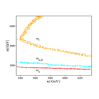
Figure 1: The available spaces for the quark masses $m_{u,d,s}$ under the constraints from the experimental values of the decay constants $f_{\pi}$ and $f_{K}$.

We choose $(A=0;B=1)$, repeat the previous steps, and obtain that the mass of quarks $[m_{u,d},m_{s}]$ is $[100,220]$ in $\rm{MeV}$.

Using the holographic LFWF, the kaon radius observable is predicted for two sets $(A=1;B=1)$ and $(A=0;B=1)$. This observable is sensitive to long-distance (LD; nonperturbative) physics. The root-mean-square kaon radius is given by BroTera6

$$r_{K}=\left[\frac{3}{2}\int d^{2}{\mathbf{r}}\,d\alpha~{}(r\bar{\alpha})^{2}|\Psi^{K}(r,\alpha)|^{2}\right]^{1/2}\,,$$ (31)

where

$$|\Psi^{K}(r,\alpha)|^{2}=\sum_{h,\bar{h}}|\Psi^{K}_{h,\bar{h}}(r,\alpha)|^{2}.$$ (32)

Our predictions for $r_{K}$ are presented in Table 1. As can be seen, we get a better agreement with the experimental value for the spin-improved LFWF using set I. Our prediction for set II is closer to that via the lattice QCD.

Table 1: Predictions for $K$ meson radius via the lattice QCD and AdS/QCD correspondence.

	Ours $(A=1;B=1)$	Ours $(A=0;B=1)$	Lattice QCD Aoki	Exp pdgk
Value (fm)	$0.52\pm 0.07$	$0.63\pm 0.09$	0.62	$0.56\pm 0.03$

For a better analysis of the holographic LFWF, we investigate the behavior of the EM form factor for the $K$ meson in the AdS/QCD approach. The kaon EM form factor is defined as

$$\langle K(p)|J^{EM}_{\mu}(0)|K(p^{\prime})\rangle=2\,(p+p^{\prime})_{\mu}F_{K}(Q^{2}),$$ (33)

where $(p-p^{\prime})^{2}=-Q^{2}$. The EM current is $J^{EM}_{\mu}=\frac{2}{3}\,\bar{u}(0)\gamma_{\mu}\,u(0)-\frac{1}{3}\,\bar{s}(0)\gamma_{\mu}\,s(0)$. The EM form factor can be expressed in terms of the LFWF as Drell ; West

$$F_{K}(Q^{2})=\int\,d^{2}{\mathbf{r}}\,d\alpha\,J_{0}[(r\bar{\alpha})Q]|\Psi^{K}(r,\alpha)|^{2}.$$ (34)

Our predictions and the experimental data Amendolia for the EM form factor of the $K$ meson with respect to $Q^{2}$, in the interval $0.10\,\rm{GeV}^{2}\leq Q^{2}\leq 1\,\rm{GeV}^{2}$, are shown in Fig. (2).

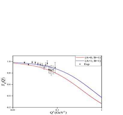
Figure 2: Our predictions and experimental data for the EM form factor of the $K$ meson.

As can be seen, our predictions for two sets are in a satisfactory agreement with the experimental data.

Figure 3 shows the holographic twist-2 DA $\phi_{{}_{K}}(\alpha,\mu)$ with respect to $\alpha$, obtained form Eqs. (II), on which red and blue lines show the results for two sets in $\mu=1~{}\rm{GeV}$, respectively. In this figure, we compare the holographic twist-2 DA with the prediction of the LCSR. It can be seen that $\phi_{{}_{K}}(\alpha)$ for set II is broader than both predictions for set I and the LCSR.

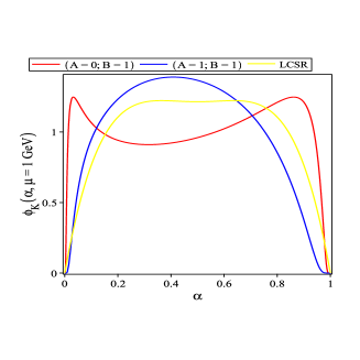
Figure 3: The results for $\phi_{K}$ at $\mu=1~{}\rm{GeV}$ with the AdS/QCD and LCSR.

The moments $\langle\xi_{n}\rangle$ and inverse moment $\left\langle{\alpha}^{-1}\right\rangle$ can be investigated based on the twist-2 DA $\phi_{{}_{K}}(\alpha,\mu)$ as

$$\langle\xi_{n}\rangle = \int_{0}^{1}d\alpha(2\alpha-1)^{n}\phi_{{}_{K}}(\alpha,\mu),$$

$$\left\langle{\alpha}^{-1}\right\rangle = \int_{0}^{1}d\alpha\frac{\phi_{{}_{K}}(\alpha,\mu)}{\alpha}\,.$$ (35)

By using the holographic DA $\phi_{{}_{K}}(\alpha,\mu)$, we calculate $\langle\xi_{2}\rangle$, $\langle\xi_{4}\rangle$, and $\langle{\alpha}^{-1}\rangle$ and compare them with the predictions of some nonperturbative methods such as the light-front quark model (LFQM), lattice QCD, and LCSR. Our results are presented in Table 2.

Table 2: Prediction values for $\langle\xi_{2}\rangle$, $\langle\xi_{4}\rangle$, and $\langle{\alpha}^{-1}\rangle$ via some methods.

DA	$\mu$ [GeV]	$\langle\xi_{2}\rangle$	$\langle\xi_{4}\rangle$	$\langle\alpha^{-1}\rangle$
Ours $(A=1;B=1)$	$1$	$0.21\pm 0.02$	$0.09\pm 0.01$	$3.54\pm 0.42$
Ours $(A=0;B=1)$	$1$	$0.32\pm 0.04$	$0.18\pm 0.02$	$5.33\pm 0.74$
LFQM Choi	$1$	$0.21$	$0.09$	–
LFQM Chung92	$1$	$0.20$	$0.08$	–
Lattice nam17	$1$	$0.20$	0.09	–
Lattice Braun6	$2$	$0.26$	–	–
LCSR Ball5	$2$	$0.26\pm 0.04$	–	–
Instanton vacuum nam6	$1$	$0.18$	$0.07$	–

Our predictions for $\langle\xi_{2}\rangle$ and $\langle\xi_{4}\rangle$ in set I are nearly equal to those of the LFQM and lattice QCD for $\mu=1~{}\rm{GeV}$.

To evaluate the differential branching ratio of the $B\to K\mu^{+}\mu^{-}$ transition on $q^{2}$, we need to calculate the transition form factors. The explicit expressions of these form factors in terms of the light-cone DAs are given in Ref. Aliev1 . We use these expressions and replace the holographic DAs in them; then we convert the obtained form factors based on the following definitions, which are more conventional Bailey :

$$\langle K(p)|\bar{s}\,\gamma_{\mu}\,b|B(p_{B})\rangle = P_{\mu}\,f_{+}(q^{2})+q_{\mu}\,\frac{m_{B}^{2}-m_{K}^{2}}{q^{2}}\,[f_{-}(q^{2})-f_{+}(q^{2})],$$

$$\langle K(p)|\bar{s}\,i\,\sigma_{\mu\nu}\,q^{\nu}\,(1+\gamma_{5})\,b|B(p_{B})\rangle = \,[P_{\mu}\,q^{2}-(m_{B}^{2}-m_{K}^{2})\,q_{\mu}]\,\frac{f_{{}_{T}}}{m_{B}+m_{K}}.$$ (36)

In these definitions, $p$ and $p_{B}$ refer to the momentums of the $K$ and $B$ meson, respectively; $q=p_{B}-p$ is the momentum carried by leptons and $P=p_{B}+q$.

Usually, the numerical results for the form factors calculated via different methods in QCD have a cutoff. So, to evaluate the form factors for the whole physical region $m_{\ell}^{2}\leq q^{2}\leq(m_{B}-m_{K})^{2}$, we look for a good parametrization of the form factors in such a way that, in the large values of $q^{2}$, this parametrization can coincide with the lattice predictions Bailey . Our numerical calculations show that the sufficient parametrization of the form factors with respect to $q^{2}$ is as follows:

$$F(q^{2})=\frac{1}{1-(\frac{q^{2}}{m_{B}^{2}})}\sum_{r=0}^{2}b_{r}\left[z^{r}+(-1)^{r}\,\frac{r}{3}\,z^{4}\right]\,,$$ (37)

where $z=\frac{\sqrt{t_{+}-q^{2}}-\sqrt{t_{+}-t_{0}}}{\sqrt{t_{+}-q^{2}}+\sqrt{t_{+}-t_{0}}}$, $t_{+}=(m_{B}+m_{K})^{2}$, and $t_{0}=(m_{B}+m_{K})(\sqrt{m_{B}}-\sqrt{m_{K}})^{2}$ Bourrely . Table 3 shows the values of $b_{r}~{}(r=0,...,2)$ for the form factors.

Table 3: Results of $z$-expansion fits of the $B\to K$ form factors.

$(A=1;B=1)$	$b_{0}$	$b_{1}$	$b_{2}$	$(A=0;B=1)$	$b_{0}$	$b_{1}$	$b_{2}$
$f_{+}$	0.43	-1.13	-0.21	$f_{+}$	0.38	-1.54	-0.85
$f_{-}$	0.27	0.08	-0.25	$f_{-}$	0.24	-0.31	-1.01
$f_{T}$	0.45	-0.99	0.12	$f_{T}$	0.40	-1.50	-0.41

Figure 4 shows the results for the $f_{+},f_{-}$, and $f_{T}$ form factor in two sets. In this figure, circles show the lattice predictions in the large values of $q^{2}$.

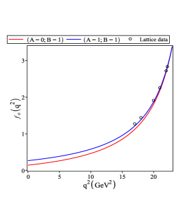
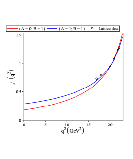
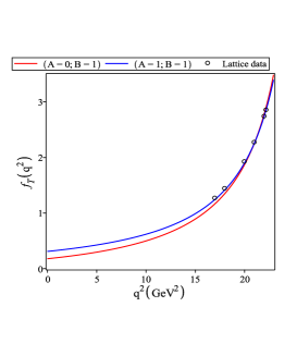
Figure 4: The form factor $f_{+},f_{-}$ and $f_{T}$ of the $B\to K$ decay on $q^{2}$. Circles show the lattice data in large $q^{2}$.

Now, we can evaluate the differential branching ratio of the $B\to K\mu^{+}\mu^{-}$ transition on $q^{2}$. The transition of the $B$ meson to the final state $K\mu^{+}\mu^{-}$ receives contributions from tree level decays and decays mediated through virtual quantum loop processes. The tree level decays proceed through the decay of a $B$ meson to a vector $c\bar{c}$ resonance and a $K$ meson, followed by the decay of the resonance to a pair of muons. Decays mediated by FCNC loop processes give rise to pairs of muons with a nonresonant mass distribution. A broad peaking structure is observed in the dimuon spectrum of $B\to K\mu^{+}\mu^{-}$ decay in the kinematic region where the kaon has a low recoil against the dimuon system Aaij4 .

In the SM, the semileptonic decays such as the $B\to K\ell^{+}\ell^{-}$ transitions that occur via $b\to s~{}\ell^{+}\ell^{-}$ transition, are described by the effective Hamiltonian as

$$H_{\rm eff}=-\frac{G_{F}}{\sqrt{2}}V_{tb}V_{ts}^{*}\sum_{i=1}^{10}C_{i}(\mu)O_{i}(\mu)\,,$$ (38)

where $V_{tb}$ and $V_{ts}$ are the elements of the CKM matrix, and $C_{i}(\mu)$ are the Wilson coefficients. The standard set of the local operators $O_{i}(\mu)$ is found, for example, in Ref. Buras0 . The most relevant contributions to $b\to s~{}\ell^{+}\ell^{-}$ transitions are (a) the tree level operators $O_{1,2}$, (b) the penguin operator $O_{7}$, and (c) the box operators $O_{9,10}$. The current-current operators $O_{1,2}$ involve an intermediate charm loop coupled to the lepton pair via the virtual photon (see Fig. 1). The electroweak penguin operators $O_{7}$, and $O_{9,10}$ are responsible for the short-distance (SD) effects in the FCNC $b\to s$ transition, but the operators $O_{1,2}$ involve both SD and LD contributions in this transition. In the naive factorization approximation, contributions of the $O_{1,2}$ operators have the same form factor dependence as $C_{9}$ and can, therefore, be absorbed into an effective Wilson coefficient $C^{\rm eff}_{9}$ Lyon .

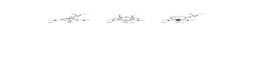
Figure 5: (a) and (b) $O_{7}$ and $O_{9,10}$ short-distance contributions. (c) $O_{1,2}$ long-distance charm-loop contribution.

Therefore, the effective Wilson coefficient $C_{9}^{\rm{eff}}$ is given as $C^{\rm eff}_{9}=C_{9}+Y_{SD}(q^{2})+Y_{LD}(q^{2})$, where $Y_{SD}(q^{2})$ describes the SD contributions from four-quark operators far away from the resonance regions. The LD contributions, $Y_{LD}(q^{2})$ from four-quark operators near the $c\bar{c}$ resonances cannot be calculated from the first principles of QCD and are usually parametrized in the form of a phenomenological Breit-Wigner formula as Buras0

$$Y_{LD}(q^{2}) = \frac{3\pi}{\alpha^{2}}\sum_{V_{i}=\psi(1s),\psi(2s)}\frac{\Gamma(V_{i}\to l^{+}l^{-})m_{V_{i}}}{m_{V_{i}}^{2}-q^{2}-im_{V_{i}}\Gamma_{V_{i}}}.$$ (39)

The expressions of the differential decay width $d\Gamma/dq^{2}$ for the $B\to K\,l^{+}\,l^{-}$ can be found in Bourrely . This expression contains the CKM matrix elements, Wilson coefficients, and form factors related to the definitions in Eq. (III). In this paper, we take $C_{7}^{\rm eff}=-0.313$, $C_{10}=-4.669$ Faessler and use $C_{9}^{\rm eff}$ according to Ref. Buras0 . Considering two charm resonances, $\psi(1s)$ and $\psi(2s)$, the dependency of the differential branching ratio for the $B\to K\mu^{+}\mu^{-}$ decay on $q^{2}$ is presented in Fig. 6. In this figure, the results obtained by the LCSR Aliev1 and lattice QCD Bailey approaches are shown with yellow and green lines, respectively. Also, the experimental values Bifani with their errors are plotted in this figure.

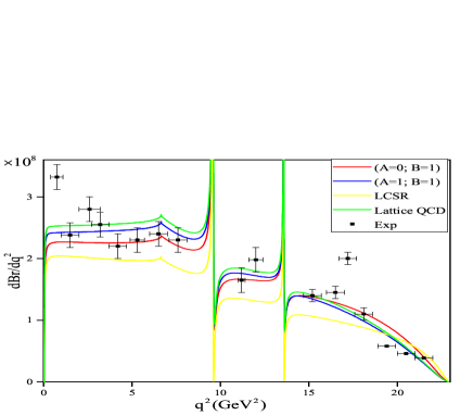
Figure 6: The differential branching ratios of the semileptonic $B\to K\mu^{+}\,\mu^{-}$ decays on $q^{2}$.

As can be seen in Fig. 6, the predictions of all models for the differential branching ratio of the $B\to K\mu^{+}\mu^{-}$ transition on $q^{2}$ are not in a good agreement with the experimental value in the low energy region ($q^{2}<1~{}\rm GeV^{2}$) where the nonperturbative QCD overcomes. For the momentum transfer squared between $1~{}\rm GeV^{2}<q^{2}<10~{}\rm GeV^{2}$, a large number of the experimental values (central values) are between our predictions via the AdS/QCD correspondence for two sets. In the high momentum transfer squared region $(q^{2}>10~{}\rm GeV^{2})$, the predictions of the lattice QCD and AdS/QCD for two sets, are well fitted to experimental values (by considering their errors).

To summarize, based on the dynamical spin effects, we extracted the twist-$2$, $-3$, and $-4$ DAs of the $K$ pseudoscalar meson in the AdS/QCD correspondence approach. The AdS/QCD scale $\kappa=590~{}\rm{MeV}$; this value is provide by fitting it to the Regge slopes, and two sets $(A=1;B=1)$ and $(A=0;B=1)$ for the dynamical spin effects were used in our analysis. For a better analysis, we calculated the masses of the light quarks with the help of the experimental values for the decay constants of pion and kaon pseudoscalar mesons in two sets. The radius, and the EM form factor of the $K$ meson, quantities related to the holographic LFWF $\Psi^{K}(r,\alpha)$, were investigated and compared with the lattice QCD and experimental values. By evaluating the transition form factors with the help of the holographic DAs, the differential branching ratio for the $B\to K\mu^{+}\mu^{-}$ decay on $q^{2}$ was plotted for two sets of $A$ and $B$. A comparison with the experimental values showed that our predictions with the AdS/QCD correspondence were good.

References

(1)
J. T. Wei et al. (Belle Collaboration), Phys. Rev. Lett. 103, 171801 (2009).
(2)
T. Aaltonen et al. (CDF Collaboration), Phys. Rev. Lett. 106, 161801 (2011).
(3)
T. Aaltonen et al. (CDF Collaboration), Phys. Rev. Lett. 107, 201802 (2011).
(4)
J. P. Lees et al. (BABAR Collaboration), Phys. Rev. D 86, 032012 (2012).
(5)
R. Aaij et al. (LHCb Collaboration), J. High Energy Phys.
07 (2012) 133.
(6)
R. Aaij et al. (LHCb Collaboration), J. High Energy Phys.
02 (2013) 105.
(7)
R. Aaij et al. (LHCb collaboration), J. High Energy Phys.
06 (2014) 133.
(8)
S. Bifani et al, arXiv: 1705.02693 [hep-ex].
(9)
C. Bouchard, G. P. Lepage, C. Monahan, H. Na, and J. Shigemitsu
(HPQCD Collaboration), Phys. Rev. D 88, 054509 (2013).
(10)
J. A. Bailey et al. Phys. Rev. D 93, 025026 (2016).
(11)
V. L. Chernyak and I. R. Zhitnitsky, Phys. Rep. C 112, 173
(1984).
(12)
V. M. Belyaev, A. Khodjamirian, and R. Ruckl, Z. Phys. C 60,
349 (1993).
(13)
C. W. Hwang, Phys. Rev. D 86, 014005
(2012).
(14)
M. Ahmady and R. Sandapen, Phys. Rev. D 87,
054013 (2013).
(15)
M. Ahmady, R. Campbell, S. Lord, and R. Sandapen, Phys. Rev. D 88, 074031 (2013).
(16)
M. Ahmady, R. Campbell, S. Lord, and R. Sandapen, Phys. Rev. D 88, 014042 (2014).
(17)
Q. Chang, S. J. Brodsky, and X. Q. Li, Phys. Rev. D 95, 094025
(2017).
(18)
M. R. Ahmady, S. Lord, and R. Sandapen, Phys. Rev. D 90,
074010 (2014).
(19)
M. Ahmady, F. Chishtie, and R. Sandapen, Phys. Rev. D 95,
074008 (2017).
(20)
V.M. Braun and I.B. Filyanov, Z. Phys. C 44,
157 (1989).
(21)
V. M. Belyaev, V. M. Braun, A. Khodjamirian, and R. Ruckl, Phys.
Rev. D 51, 6177 (1995).
(22)
J. R. Forshaw and R. Sandapen, J. High Energy Phys. 10 (2011)
093.
(23)
J. B. Kogut and L. Susskind, Phys. Rev. D 9, 3391 (1974).
(24)
M. Diehl, Eur. Phys. J. C 25, 223 (2002).
(25)
T. Heinzl, Lect. Notes Phys. 572, 55 (2001); T. Heinzl, Nucl.
Phys. B, Proc. Suppl. 90, 83 (2000).
(26)
H. M. Choi and C. R. Ji, Phys. Rev. D 75, 034019 (2007).
(27)
A. P. Trawiski, Few Body Syst. 57, 449 (2016).
(28)
G. P. Lepage and S. J. Brodsky, Phys. Rev. D 22, 2157 (1980).
(29)
G. F. de Teramond and S. J. Brodsky, Phys. Rev.
Lett. 102, 081601 (2009).
(30)
A. Karch, E. Katz, D. T. Son, and M. A. Stephanov,
Phys. Rev. D 74, 015005 (2006).
(31)
S. J. Brodsky, G. F. de Teramond, H. G. Dosch, and J. Erlich, Phys.
Rep. 584, 1 (2015).
(32)
S. J. Brodsky and G. F. de Teramond, Subnucl. Ser. 45, 139
(2009).
(33)
S. J. Brodsky and G. F. de Teramond, Phys. Rev. D 77, 056007
(2008).
(34)
S. Aoki et al. Phys. Rev. D 93, 034504 (2016).
(35)
S. Eidelman et al (Particle Data Group), Phys. Lett. B
592, 1 (2004).
(36)
S. D. Drell and T. M. Yan, Phys. Rev. Lett. 24, 181 (1970).
(37)
G. B. West, Phys. Rev. Lett. 24, 1206 (1970).
(38)
S. R. Amendolia et al. Phys. Lett. B 178, 435 (1986).
(39)
C. R. Ji, P. L. Chung, and S. R. Cotanch, Phys. Rev. D 45,
4214 (1992).
(40)
S. i. Nam, arXiv, Mod. Phys. Lett. A 32, 1750218 (2017).
(41)
V. M. Braun et al, Phys. Rev. D 74, 074501 (2006).
(42)
P. Ball and R. Zwicky, Phys. Rev. D 71, 014015 (2005).
(43)
S. i. Nam, H. C. Kim, A. Hosaka, and M. M. Musakhanov, Phys. Rev D
74, 014019 (2006).
(44)
T. M. Aliev, A. Ozpineci, M. Savci, and H. Koru, Phys. Lett. B 400, 194 (1997).
(45)
C. Bourrely, I. Caprini, and L. Lellouch, Phys. Rev. D 79,
013008 (2009).
(46)
R. Aaij et al. (LHCb collaboration), Phys. Rev. Lett. 111, 112003 (2013).
(47)
A. J. Buras and M. Muenz, Phys. Rev. D 52, 186 (1995).
(48)
J. Lyon and R. Zwicky, arXiv:1406.0566 [hep-ph].
(49)
A. Faessler, Th. Gutsche, M. A. Ivanov, J. G. Korner, and V. E.
Lyubovitskij, Eur. Phys. J. C 4, 18 (2002).