SDPNAL$+$: A Matlab software for semidefinite programming with bound constraints (version 1.0)

Abstract. Sdpnal$+$ is a Matlab software package that implements an augmented Lagrangian based method to solve large scale semidefinite programming problems with bound constraints. The implementation was initially based on a majorized semismooth Newton-CG augmented Lagrangian method, here we designed it within an inexact symmetric Gauss-Seidel based semi-proximal ADMM/ALM (alternating direction method of multipliers/augmented Lagrangian method) framework for the purpose of deriving simpler stopping conditions and closing the gap between the practical implementation of the algorithm and the theoretical algorithm. The basic code is written in Matlab, but some subroutines in C language are incorporated via Mex files. We also design a convenient interface for users to input their SDP models into the solver. Numerous problems arising from combinatorial optimization and binary integer quadratic programming problems have been tested to evaluate the performance of the solver. Extensive numerical experiments conducted in [Yang, Sun, and Toh, Mathematical Programming Computation, 7 (2015), pp. 331–366] show that the proposed method is quite efficient and robust, in that it is able to solve 98.9% of the 745 test instances of SDP problems arising from various applications to the accuracy of $10^{-6}$ in the relative KKT residual.

Keywords: Semidefinite programming, Augmented Lagrangian, Semismooth Newton-CG method, Matlab software package.

1 Introduction

Let $\mathbb{S}^{n}$ be the space of $n\times n$ real symmetric matrices and $\mathbb{S}^{n}_{+}$ be the cone of positive semidefinite matrices in $\mathbb{S}^{n}$. For any $X\in\mathbb{S}^{n}$, we may sometimes write $X\succeq 0$ to indicate that $X\in\mathbb{S}^{n}_{+}$. Let ${\cal P}=\{X\in\mathbb{S}^{n}:L\leq X\leq U\}$, where $L,U$ are given $n\times n$ symmetric matrices whose elements are allowed to take the values $-\infty$ and $+\infty$, respectively. Consider the semidefinite programming (SDP) problem:

$$({\rm\bf SDP})\quad\min\Big{\{}\langle C,\,X\rangle\mid{\cal A}(X)=b,\;l\leq{\cal B}(X)\leq u,\;X\in\mathbb{S}^{n}_{+},\;X\in{\cal P}\Big{\}},$$

where $b\in\mathbb{R}^{m}$, and $C\in\mathbb{S}^{n}$ are given data, ${\cal A}:\mathbb{S}^{n}\rightarrow\mathbb{R}^{m}$ and ${\cal B}:\mathbb{S}^{n}\rightarrow\mathbb{R}^{p}$ are two given linear maps whose adjoints are denoted as ${\cal A}^{*}$ and ${\cal B}^{*}$, respectively. The vectors $l,u$ are given $p$-dimensional vectors whose elements are allowed to take the values $-\infty$ and $\infty$, respectively. Note that ${\cal P}=\mathbb{S}^{n}$ is allowed, in which case there are no additional bound constraints imposed on $X$. We assume that the $m\times m$ symmetric matrix ${\cal A}{\cal A}^{*}$ is invertible, i.e., ${\cal A}$ is surjective.

Note that (SDP) is equivalent to

$$({\rm P})\quad\min\Big{\{}\langle C,\,X\rangle\mid{\cal A}(X)=b,\;{\cal B}(X)-s=0,\;X\in\mathbb{S}^{n}_{+},\;X\in{\cal P},\;s\in{\cal Q}\Big{\}},$$

where ${\cal Q}=\{s\in\mathbb{R}^{p}:l\leq s\leq u\}$. The dual of (P), ignoring the minus sign in front of the minimization, is given by

$$({\rm D})\;\min\left\{\delta_{{\cal P}}^{*}(-Z)+\delta_{{\cal Q}}^{*}(-v)+\langle-b,\,y\rangle\;\Big{|}\;\begin{array}[]{l}{\cal A}^{*}(y)+{\cal B}^{*}(\bar{y})+S+Z=C,\;-\bar{y}+v=0,\\[3.0pt] S\in\mathbb{S}^{n}_{+},\;Z\in\mathbb{S}^{n},\;y\in\mathbb{R}^{m},\;\bar{y}\in\mathbb{R}^{p},\;v\in\mathbb{R}^{p}\end{array}\right\},$$

where for any $Z\in\mathbb{S}^{n}$, $\delta_{{\cal P}}^{*}(-Z)$ is defined by

$$\delta_{{\cal P}}^{*}(-Z)=\sup\{\langle-Z,\,W\rangle\mid W\in{\cal P}\}$$

and $\delta_{{\cal Q}}^{*}(\cdot)$ is defined similarly. We note that our solver is designed based on the assumption that (P) and (D) are feasible.

While we have presented the problem (SDP) with a single variable block $X$, our solver is capable of solving the following more general problem with $N$ blocks of variables:

$$\begin{array}[]{ll}\min&\sum_{j=1}^{N}\langle C^{(j)},\,X^{(j)}\rangle\\[5.0pt] \mbox{s.t.}&\sum_{j=1}^{N}{\cal A}^{(j)}(X^{(j)})=b,\quad l\leq\sum_{j=1}^{N}{\cal B}^{(j)}(X^{(j)})\leq u,\\[5.0pt] &X^{(j)}\in{\cal K}^{(j)},\;X^{(j)}\in{\cal P}^{(j)},\;j=1,\ldots,N,\end{array}$$ (5)

where ${\cal A}^{(j)}:{\cal X}^{(j)}\to\mathbb{R}^{m}$, and ${\cal B}^{(j)}:{\cal X}^{(j)}\to\mathbb{R}^{p}$ are given linear maps, ${\cal P}^{(j)}:=\{X^{(j)}\in{\cal X}^{(j)}\mid L^{(j)}\leq X^{(j)}\leq U^{(j)}\}$ and $L^{(j)},U^{(j)}\in{\cal X}^{(j)}$ are given symmetric matrices where the elements are allowed to take the values $-\infty$ and $\infty$, respectively. Here ${\cal X}^{(j)}=\mathbb{S}^{n_{j}}$ ($\mathbb{R}^{n_{j}}$), and ${\cal K}^{(j)}={\cal X}^{(j)}$ or ${\cal K}^{(j)}=\mathbb{S}^{n_{j}}_{+}$ ($\mathbb{R}^{n_{j}}_{+}$). For later expositions, we should note that when ${\cal X}^{(j)}=\mathbb{S}^{n_{j}}$, the linear map ${\cal A}^{(j)}:\mathbb{S}^{n_{j}}\to\mathbb{R}^{m}$ can be expressed in the form of

$${\cal A}^{(j)}(X^{(j)})=\left[\begin{array}[]{c}\langle A^{(j)}_{1},\,X^{(j)}\rangle,\ldots,\langle A^{(j)}_{m},\,X^{(j)}\rangle\end{array}\right]^{T},$$ (7)

where $A^{(j)}_{1},\ldots,A^{(j)}_{m}\in\mathbb{S}^{n_{j}}$ are given constraint matrices. The corresponding adjoint $({\cal A}^{(j)})^{*}:\mathbb{R}^{m}\to\mathbb{S}^{n_{j}}$ is then given by

$$\begin{array}[]{l}({\cal A}^{(j)})^{*}y=\sum_{k=1}^{m}y_{k}A^{(j)}_{k}.\end{array}$$

In this paper, we introduce our Matlab software package Sdpnal$+$ for solving (SDP) or more generally (5), where the maximum matrix dimension is assumed to be moderate (say less than 5000) but the number of linear constraints $m+p$ can be large (say more than a million). One of our main contributions here is that the current algorithm has substantially extended the capability of Sdpnal$+$ to solve the general problem (5) compared to the original version in [24], wherein the algorithm is designed to solve a problem with only linear equality constraints and ${\cal P}=\{X\in\mathbb{S}^{n}\mid X\geq 0\}$ or ${\cal P}=\mathbb{S}^{n}$. Moreover, the implementation in [24] was based on a majorized semismooth Newton-CG augmented Lagrangian method developed in that paper. Here, for the purpose of deriving simpler stopping conditions, we redesign the algorithm by employing an inexact semi-proximal alternating direction method of multipliers (sPADMM) (or the semi-proximal augmented Lagrangian (sPALM) if the bound constraints are absent) framework developed in [2] for multi-block convex composite conic programming problems. Currently, the algorithm which we have implemented is a $2$-phase algorithm based on the augmented Lagrangian function for (D). In the first phase, we employ the inexact symmetric Gauss-Seidel based sPADMM to solve the problem to a modest level of accuracy. Note that while the main purpose of the first phase algorithm is to generate a good initial point to warm-start the second phase algorithm, it can be used on its own to solve a problem. The algorithm we have implemented in the second phase is an inexact sPADMM for which the main subproblem in each iteration is solved by a semismooth Newton-CG method.

The development of Sdpnal$+$ in [24], which is built on the earlier work on Sdpnal in [25], has in fact spurred much of the recent progresses in designing efficient convergent ADMM-type algorithms for solving multi-block convex composite conic programming, such as [2, 7, 16]. Those works in turn shaped the recent algorithmic design of Sdpnal$+$. Indeed, the algorithm in the first phase of Sdpnal$+$ is the same as the convergent ADMM-type method developed in [16] when the subproblems in each iteration are solved analytically. For the algorithm in the second phase, it is an economical variant of the majorized semismooth Newton-CG (SNCG) augmented Lagrangian method designed in [24] to solve (D) for which only one SNCG subproblem is solved in each iteration.

Another contribution of this paper is our development of a basic interface for the users to input their SDP models into the Sdpnal$+$ solver. While there are currently two well developed matlab based user interfaces for SDP problems, namely, CVX [4] and YALMIP [9], there are strong motivations for us to develop our own interface here. A new interface is necessary to facilitate the modeling of an SDP problem for Sdpnal$+$ because of latter’s flexibility to directly accept inequality constraints of the form “$l\leq{\cal B}(X)\leq u$”, and bound constraints of the form “$L\leq X\leq U$”. The flexibility can significantly simplify the generation of the data in the Sdpnal$+$ format as compared to what need to be done in CVX or YALMIP to reformulate them as equality constraints through introducing extra variables. In addition, the final number of equality constraints present in the data input to Sdpnal$+$ can also be substantially fewer than those present in CVX or YALMIP. It is important to note here that the number of equality constraints present in the generated problem data can greatly affect the computational efficiency of the solvers, especially for interior-point based solvers. An illustration of the benefits just mentioned will be given at the end of Section 5.

Our Sdpnal$+$ solver is designed for solving feasible problems of the form presented in (P) and (D). It is capable of solving large scale SDPs with $m$ or $p$ up to a few millions but $n$ is assumed to be moderate (up to a few thousands). Extensive numerical experiments conducted in [24] show that a variety of large scale SDPs can be solved by Sdpnal$+$ much more efficiently than the best alternative methods [10, 21].

The Sdpnal$+$ package can be downloaded from the following website:

http://www.math.nus.edu.sg/m̃attohkc/SDPNALplus.html

Installation and general information such as citations, can be found at the above link. The test instances which we have used to evaluate the performance of our solver can also be found at the above website.

We have evaluated the performance of Sdpnal$+$ on various classes of large scale SDP problems arising from the relaxation of combinatorial problems such as maximum stable set problems, quadratic assignment problems, frequency assignment problems, and binary integer quadratic programming problems. The solver has also been tested on large SDP problems arising from robust clustering problems, rank-one tensor approximation problems, as well as electronic structure calculations in quantum chemistry. The detailed numerical results can be found at the above website. Based on the numerical evaluation of Sdpnal$+$ on 745 SDP problems, we can observe that the solver is fairly robust (in the sense that it is able to solve most of the tested problems to the accuracy of $10^{-6}$ in the relative KKT residual) and highly efficient in solving the tested classes of problems.

The remaining parts of this paper are organized as follows. In the next section, we describe the installation and present some general information on our software. Section 2 gives some details on the main solver function sdpnalplus.m. In Section 3, we describe the algorithm implemented in Sdpnal$+$ and discuss some implementation issues. In Section 4, we present a basic interface for the users to input their SDP models into the Sdpnal$+$ solver. In Section 5,

we present a few SDP examples to illustrate the usage of our software, and how to input the SDP models into our interface. Section 6 gives a summary of the numerical results obtained by Sdpnal$+$ in solving 745 test instances of SDP problems arising from various sources. Finally, we conclude the paper in Section 7.

2 Data structure and main solver

Sdpnal$+$ is an enhanced version of the Sdpnal solver developed by Zhao, Sun and Toh [25]. The internal implementation of Sdpnal$+$ thus follows the data structures and design framework of Sdpnal. A casual user need not understand the internal implementation of Sdpnal$+$ ​​.

2.1 The main function: sdpnalplus.m

In the Sdpnal$+$ solver, the main routine is sdpnalplus.m, whose calling syntax is as follows:

[obj,X,s,y,S,Z,ybar,v,info,runhist] = ...
     sdpnalplus(blk,At,C,b,L,U,Bt,l,u,OPTIONS,X,s,y,S,Z,ybar,v);

Input arguments.

• blk: a cell array describing the conic block structure of the SDP problem.

• At, C, b, L, U, Bt, l, u: data of the problem (SDP).
  If ${L\leq X}$ but $X$ is unbounded above, one can set U=inf or U=[]. Similarly, if the linear map ${\cal B}$ is not present, one can set Bt=[], l=[], u=[].

• OPTIONS: a structure array of parameters (optional).

• X, s, y, S, Z, ybar, v: an initial iterate (optional).

Output arguments. The names chosen for the output arguments explain their contents. The argument ${\tt X}$ is a solution to (P) which satisfies the constraints $X\in\mathbb{S}^{n}_{+}$ and $X\in{\cal P}$ approximately up to the desired accuracy tolerance. The argument info is a structure array which records various performance measures of the solver. For example

  info.etaRp, info.etaRd, info.etaK1, info.etaK2

correspond to the measures $\eta_{P}$, $\eta_{D}$, $\eta_{{\cal K}}$, $\eta_{{\cal P}}$ defined later in (10), respectively. The argument runhist is a structure array which records the history of various performance measures during the course of running sdpnalplus.m. For example,

$${\tt runhist.primobj},\;\;{\tt runhist.dualobj},\;\;{\tt runhist.relgap}$$

$${\tt runhist.primfeasorg},\;\;{\tt runhist.dualfeasorg}$$

record the primal and dual objective values, complementarity gap, primal and dual infeasibilities at each iteration, respectively.

2.2 Generation of starting point by admmplus.m

If an initial point (X,s,y,S,Z,ybar,v) is not provided for sdpnalplus.m, we call the function admmplus.m, which implements a convergent $3$-block ADMM proposed in [16], to generate a starting point. The routine admmplus.m has a similar calling syntax as sdpnalplus.m given as follows:

[obj,X,s,y,S,Z,ybar,v,info,runhist] = ...
     admmplus(blk,At,C,b,L,U,Bt,l,u,OPTIONS,X,s,y,S,Z,ybar,v);

Note that if an initial point (X,s,y,S,Z,ybar,v) is not supplied to admmplus.m, the default initial point is (0,0,0,0,0,0,0).

We should mention that although we use admmplus.m for the purpose of warm-starting sdpnalplus.m, the user has the freedom to use admmplus.m alone to solve the problem (SDP).

2.3 Arrays of input data

The format of the input data in Sdpnal$+$ is similar to those in SDPT3 [18, 20]. For each SDP problem, the conic block structure of the problem data is described by a cell array named blk. If the $k$th block X{k} of the variable X is a nonnegative vector block with dimension $n_{k}$, then we set

1. blk{k,1} = ’l’,  blk{k,2} = $n_{k}$,

2. At{k} = [$n_{k}\times m$   sparse],   Bt{k} = [$n_{k}\times p$   sparse],

3. C{k}, L{k}, U{k}, X{k}, S{k}, Z{k} = [$n_{k}\times 1$   double or sparse].

If the $j$th block X{j} of the variable X is a semidefinite block consisting of a single block of size $s_{j}$, then the content of the $j$th block is given as follows:

1. blk{j,1} = ’s’,   blk{j,2} = $s_{j}$,

2. At{j} = [$\bar{s}_{j}\times m$   sparse ],  Bt{k} = [$\bar{s}_{j}\times p$   sparse],

3. C{j}, L{j}, U{j}, X{j}, S{j}, Z{j} = [$s_{j}\times s_{j}$   double or sparse ],

where $\bar{s}_{j}=s_{j}(s_{j}+1)/2$. By default, the contents of the cell arrays L and U are set to be empty arrays. But if ${\tt X\{j\}}\geq 0$ is required, then one can set

$$\mbox{\tt L\{j\} = 0},\quad\mbox{\tt U\{j\} = []}.$$

One can also set $L=0$ to indicate that ${\tt X\{j\}}\geq 0$ for all $j=1,\ldots,N$ in (5).

We should mention that for the sake of computational efficiency, we store all the constraint matrices associated with the $j$th semidefinite block in vectorized form as a single $\bar{s}_{j}\times m$ matrix At{j}, where the $k$th column of this matrix corresponds to the $k$th constraint matrix $A^{(j)}_{k}$, i.e.,

$${\tt At\{j\}}=[{\rm svec}(A^{(j)}_{1}),\ldots,{\rm svec}(A^{(j)}_{m})],$$

and ${\rm svec}:\mathcal{S}^{s_{j}}\rightarrow\mathbb{R}^{\bar{s}_{j}}$ is the vectorization operator on symmetric matrices defined by

$${\rm svec}(X)=[X_{11},\sqrt{2}X_{12},X_{22},\ldots,\sqrt{2}X_{1,s_{j}},\ldots,\sqrt{2}X_{s_{j}-1,s_{j}},X_{s_{j},s_{j}}]^{T}.$$ (9)

We store Bt in the same format as At. The function svec.m provided in Sdpnal$+$ can easily convert a symmetric matrix into the vector storage scheme described in (9). Note that while we store the constraint matrices in vectorized form, the semidefinite blocks in the variables X, S and Z are stored either as matrices or in vectorized forms according to the storage scheme of the input data C.

Other than inputting the data (At,b,C,L,U) of an SDP problem individually, Sdpnal$+$ also provides the functions read_sdpa.m and read_sedumi.m to convert problem data stored in the SDPA [23] and SeDuMi [15] format into our cell-array data format just described. For example, for the problem theta62.dat-s in the folder /datafiles, the user can call the m-file read_sdpa.m to load the SDP data as follows:

>> [blk,At,C,b] = read_sdpa(’./datafiles/theta62.dat-s’);
>> OPTIONS.tol = 1e-6;
>> [obj,X,s,y,S,Z,ybar,v,info,runhist] = sdpnalplus(blk,At,C,b,[],[],[],[],[],OPTIONS);

2.4 The structure array OPTIONS for parameters

Various parameters used in our solver sdpnalplus.m are set in the structure array OPTIONS. For details, see SDPNALplus_parameters.m. The important parameters which the user is likely to reset are described next.

1. OPTIONS.tol: accuracy tolerance to terminate the algorithm, default is $10^{-6}$.

2. OPTIONS.maxiter: maximum number of iterations allowed, default is $20000$.

3. OPTIONS.maxtime: maximum time (in seconds) allowed, default is $10000$.

4. OPTIONS.tolADM: accuracy tolerance to use for admmplus.m when generating a starting point for the algorithm in the second phase of sdpnalplus.m (default = $10^{-4}$).

5. OPTIONS.maxiterADM: maximum number of ADMM iterations allowed for generating a starting point. When there are no bound constraints on $X$ (${\cal P}=\mathbb{S}^{n}$) and no linear inequality constraints corresponding to ${\cal B}(X)$ (hence ${\cal Q}=\emptyset$), the default value is roughly equal to 200; otherwise, the default value is 2000.

6. OPTIONS.printlevel: different levels of details to print the intermediate information during the run. It can be the integers $0,1,2$, with $1$ being the default. Setting to the highest value $2$ will result in printing the complete details.

7. OPTIONS.stopoption: options to stop the solver. The default is OPTIONS.stopoption=1, for which the solver may be stopped prematurely when stagnation occurs. To prevent the solver from stopping prematurely before the required accuracy is attained, set OPTONS.stopoption=0.

8. OPTIONS.AATsolve.method: options to solve a linear system involving the coefficient matrix ${\cal A}{\cal A}^{*}$, with
   OPTIONS.AATsolve.method=’direct’ (default) or ’iterative’.
   For the former option, a linear system of the form ${\cal A}{\cal A}^{*}y=h$ is solved by the sparse Cholesky factorization, while for the latter option, it is solved by a diagonally preconditioned PSQMR iterative solver.

2.5 Stopping criteria

In Sdpnal$+$ ​​, we measure the accuracy of an approximate optimal solution $(X,s,y,\bar{y},S,Z,v)$ for (P) and (D) by using the following relative residual based on the KKT optimality conditions:

$$\eta=\max\{\eta_{P},\eta_{D},\eta_{{\cal K}},\eta_{{\cal P}}\},$$ (10)

where ${\cal K}=\mathbb{S}^{n}_{+}$,

$$\begin{array}[]{l}\eta_{P}=\max\Big{\{}\frac{\|{\cal A}(X)-b\|}{1+\|b\|},\frac{\|{\cal B}(X)-s\|}{1+\|s\|}\Big{\}},\;\eta_{D}=\max\Big{\{}\frac{\|{\cal A}^{*}(y)+{\cal B}^{*}(\bar{y})+S+Z-C\|}{1+\|C\|},\frac{\|\bar{y}-v\|}{1+\|v\|}\Big{\}},\\[8.0pt] \eta_{{\cal K}}=\frac{1}{5}\frac{\|X-\Pi_{{\cal K}}(X-S)\|}{1+\|X\|+\|S\|},\;\eta_{{\cal P}}=\frac{1}{5}\max\Big{\{}\frac{\|X-\Pi_{{\cal P}}(X-Z)\|}{1+\|X\|+\|Z\|},\frac{\|s-\Pi_{{\cal Q}}(s-v)\|}{1+\|s\|+\|v\|}\Big{\}}.\end{array}$$

Additionally, we compute the relative gap by

$$\eta_{g}=\frac{|{\tt pobj}-{\tt dobj}|}{1+\left|\tt pobj\right|+\left|\tt dobj\right|}.$$ (12)

For a given accuracy tolerance specified in OPTIONS.tol, we terminate both sdpnalplus.m and admmplus.m when

$$\eta\leq{\tt OPTIONS.tol}.$$ (13)

2.6 Caveats

There are a few points which we should emphasize on our solver.

• It is important to note that Sdpnal$+$ is a research software. It is not intended nor designed to be a general purpose software at the moment. The solver is designed based on the assumption that the primal and dual SDP problems (P) and (D) are feasible, and that Slater’s constraint qualification holds. The solver is expected to be robust if the primal and dual SDP problems are both non-degenerate at the optimal solutions. However, if either one of them, particularly if the primal problem, is degenerate or if the Slater’s condition fails, then the solver may not be able to solve the problems to high accuracy.

• Another point to note is that our solver is designed with the emphasis on handling problems with positive semidefinite variables efficiently. Little attention has been paid on optimizing the solver to handle linear programming problems.

• While in theory our solver can easily be extended to solve problems with second-order cone constraints, it is not capable of solving such problems at the moment although we plan to extend our solver to handle second-order cone programming problems in the future.

3 Algorithmic design and implementation

For simplicity, we will describe the algorithmic design for the problem (D) instead of the dual of the more general problem (5). Our algorithm is developed based on the augmented Lagrangian function for (D), which is defined as follows: given a penalty parameter $\sigma>0$, for $(Z,v,y,\bar{y})\in\mathbb{S}^{n}\times\mathbb{R}^{p}\times\times\mathbb{R}^{m}\times\mathbb{R}^{p}$, and $(X,s)\in\mathbb{S}^{n}\times\mathbb{R}^{p}$,

$$L_{\sigma}(Z,v,S,y,\bar{y};X,s)=\left\{\begin{array}[]{l}\delta_{{\cal P}}^{*}(-Z)+\delta_{{\cal Q}}^{*}(-v)+\langle-b,\,y\rangle+\delta_{\mathbb{S}^{n}_{+}}(S)-\frac{1}{2\sigma}\|X\|^{2}-\frac{1}{2\sigma}\|s\|^{2}\\[5.0pt] +\frac{\sigma}{2}\|{\cal A}^{*}(y)+{\cal B}^{*}(\bar{y})+S+Z-C+\sigma^{-1}X\|^{2}+\frac{\sigma}{2}\|v-\bar{y}+\sigma^{-1}s\|^{2}.\end{array}\right.$$

As mentioned in the Introduction, the algorithm implemented in Sdpnal$+$ is a 2-phase algorithm where the first phase is a convergent inexact sGS-sPADMM algorithm [2] whose template is described next.

First-phase algorithm. Given an initial iteration $(Z^{0},v^{0},S^{0},y^{0},\bar{y}^{0},X^{0},s^{0})$, perform the following steps in each iteration.

Step 1.

Let $R_{1}^{k}={\cal A}^{*}(y^{k})+{\cal B}^{*}(\bar{y}^{k})+S^{k}+Z^{k}-C+\sigma^{-1}X^{k}$ and $R^{k}_{2}=v^{k}-\bar{y}^{k}+\sigma^{-1}s^{k}$. Compute $(Z^{k+1},v^{k+1})=\mbox{argmin}\;L_{\sigma}(Z,v,S^{k},y^{k},\bar{y}^{k};X^{k},s^{k})$ as follows:

$$Z^{k+1} = \mbox{argmin}\big{\{}\delta_{{\cal P}}^{*}(-Z)+\frac{\sigma}{2}\|Z-Z^{k}+R_{1}^{k}\|^{2}\big{\}}=\sigma^{-1}\Pi_{{\cal P}}(\sigma(R^{k}_{1}-Z^{k}))-(R^{k}_{1}-Z^{k}),$$

$$v^{k+1} = \mbox{argmin}\big{\{}\delta_{{\cal Q}}^{*}(-v)+\frac{\sigma}{2}\|v-v^{k}+R_{2}^{k}\|^{2}\big{\}}=\sigma^{-1}\Pi_{{\cal Q}}(\sigma(R^{k}_{2}-v^{k}))-(R^{k}_{2}-v^{k}).$$

Step 2a.

Compute

$$(y^{k+1}_{\rm tmp},\bar{y}^{k+1}_{\rm tmp}) \approx \mbox{argmin}\big{\{}L_{\sigma}(Z^{k+1},v^{k+1},S^{k},y,\bar{y};X^{k},s^{k})\big{\}}.$$

For this step, we typically need to solve a large system of linear equations given by

$$\underbrace{\left[\begin{array}[]{cc}{\cal A}{\cal A}^{*}&{\cal A}{\cal B}^{*}\\[5.0pt] {\cal B}{\cal A}^{*}&{\cal B}{\cal B}^{*}+{\cal I}\end{array}\right]}_{{\cal M}}\left[\begin{array}[]{c}y\\[5.0pt] \bar{y}\end{array}\right]=\left[\begin{array}[]{l}h_{1}:=\sigma^{-1}b-{{\cal A}(S^{k}+Z^{k+1}-C+\sigma^{-1}X^{k})}\\[5.0pt] h_{2}:=v^{k+1}+\sigma^{-1}s^{k}-{\cal B}(S^{k}+Z^{k+1}-C+\sigma^{-1}X^{k})\end{array}\right].$$ (15)

In our implementation, we solve the linear system via the sparse Cholesky factorization of ${\cal M}$ if it can be computed at a moderate cost. Otherwise, we use a preconditioned CG method to solve (15) approximately so that the residual norm satisfies the following accuracy condition:

$$\sqrt{\sigma}\|[h_{1};h_{2}]-{\cal M}[y^{k+1}_{\rm tmp};\bar{y}^{k+1}_{\rm tmp}]\|\leq\varepsilon_{k},$$

where $\{\varepsilon_{k}\}$ is a predefined summable sequence of nonnegative numbers. In [24], the linear system corresponding to ${\cal M}$ is ${\cal A}{\cal A}^{*}y=h_{1}$, and it is solved by a direct method based on sparse Cholesky factorization. Here, the inexact sGS-ADMM framework [2] we have employed gives us the flexibility to solve the linear system approximately by an iterative solver such as the preconditioned conjugate gradient method, while not affecting the convergence of the algorithm. Such a flexibility is obviously critical to the computational efficiency of the algorithm when the sparse Cholesky factorization of ${\cal M}$ is impossible to compute for a very large linear system.

Step 2b.

Let $R^{k+1}_{1}={\cal A}^{*}(y^{k+1}_{\rm tmp})+{\cal B}^{*}(\bar{y}^{k+1}_{\rm tmp})+S^{k}+Z^{k+1}-C+\sigma^{-1}X^{k}$. Compute

$$S^{k+1} = \mbox{argmin}\big{\{}\delta_{\mathbb{S}^{n}_{+}}(S)+\frac{\sigma}{2}\|S-S^{k}+R_{1}^{k+1}\|^{2}\big{\}}=\Pi_{\mathbb{S}^{n}_{+}}(S^{k}-R_{1}^{k+1}).$$

Step 2c.

Let $h_{1}^{\rm new}:=h_{1}-{\cal A}(S^{k+1}-S^{k})$, and $h_{2}^{\rm new}:=h_{2}-{\cal B}(S^{k+1}-S^{k})$. Set $(y^{k+1},\bar{y}^{k+1})=(y^{k+1}_{\rm tmp},\bar{y}^{k+1}_{\rm tmp})$ if

$$\sqrt{\sigma}\left\|[h_{1}^{\rm new};{h_{2}^{\rm new}}]-{\cal M}[y^{k+1}_{\rm tmp};\bar{y}^{k+1}_{\rm tmp}]\right\|\leq 10\varepsilon_{k};$$

otherwise solve (15) with the vector $h_{1}$ replaced by $h_{1}^{\rm new}$ and $h_{2}$ replaced by $h_{2}^{\rm new}$, and the approximate solution $(y^{k+1},\bar{y}^{k+1})$ should satisfy the above accuracy condition.

Step 3.

Let $R_{D,1}^{k+1}={\cal A}^{*}(y^{k+1})+{\cal B}^{*}(\bar{y}^{k+1})+S^{k+1}+Z^{k+1}-C$ and $R^{k+1}_{D,2}=v^{k+1}-\bar{y}^{k+1}$. Compute

$$X^{k+1}=X^{k}+\tau\sigma R^{k+1}_{D,1},\;s^{k+1}=s^{k}+\tau\sigma R^{k+1}_{D,2},$$

where $\tau\in(0,(1+\sqrt{5})/2)$ is the steplength which is typically chosen to be 1.618.

We note that by [2], the computation in Step 2a–2c is equivalent to solving the subproblem:

$$(S^{k+1},y^{k+1},\bar{y}^{k+1})=\mbox{argmin}\left\{\begin{array}[]{l}{L_{\sigma}(Z^{k+1},v^{k+1},S,y,\bar{y};X^{k},s^{k})}\\[5.0pt] +\frac{\sigma}{2}\|(S;y;\bar{y})-(S^{k};y^{k};\bar{y}^{k})\|^{2}_{{\cal H}}\end{array}\right\},$$

where ${\cal H}$ is the symmetric Gauss-Seidel decomposition linear operator associated with the linear operator $({\cal I};{\cal A};{\cal B})({\cal I},{\cal A}^{*},{\cal B}^{*})+{\rm diag}(0,0,{\cal I})$, i.e.,

$${\cal H}=\left[\begin{array}[]{ccc}({\cal A}^{*},\,{\cal B}^{*}){\cal D}^{-1}({\cal A};{\cal B})&0&0\\[5.0pt] 0&0&0\\[5.0pt] 0&0&0\end{array}\right]\quad{\mbox{with}}\;\;{\cal D}=\left[\begin{array}[]{cc}{\cal A}{\cal A}^{*}&{\cal A}{\cal B}^{*}\\ {\cal B}{\cal A}^{*}&{\cal B}{\cal B}^{*}+{\cal I}\end{array}\right].$$

There are numerous implementation issues which are addressed in Sdpnal$+$ to make the above skeletal algorithm practically efficient and robust. A detailed description of how the issues are addressed is beyond the scope of this paper. Hence we shall only briefly mention the most crucial ones.

1. Dynamic adjustment of the penalty parameter $\sigma$, which is equivalent to restarting the algorithm with a new parameter by using the most recent iterate as the initial starting point.

2. Initial scaling of the data, and dynamic scaling of the data.

3. The efficient implementation of the PCG method to compute an approximate solution for (15).

4. Efficient computation of the iterate $S^{k+1}$ by using partial eigenvalue decomposition whenever it is expected to be more economical than a full eigenvalue decomposition.

5. Efficient evaluation of the residual measure $\eta$ defined in (10).

The algorithm in the second phase of Sdpnal$+$ is designed based on the following convergent inexact sPADMM algorithm (or the sPALM algorithm if the bound constraints are absent). After presenting the algorithm, we will explain the changes we made in this algorithm compared to that developed in [24].

Second-phase algorithm. Given an initial iterate $(Z^{0},v^{0},S^{0},y^{0},\bar{y}^{0},X^{0},s^{0})$ generated in the first phase, perform the following steps in each iteration.

Step 1.

Compute $(Z^{k+1},v^{k+1})$ as in Step 1 of the first-phase algorithm.

Step 2.

Compute

$$(y^{k+1},\bar{y}^{k+1},S^{k+1})\approx\mbox{argmin}\,L_{\sigma}(Z^{k+1},v^{k+1},S,y,\bar{y};X^{k},s^{k})$$

by using the semismooth Newton-CG (SNCG) method which has been described in detail in [25] such that the following accuracy condition is met:

$$\sqrt{\sigma}\max\{\|b-{\cal A}\Pi_{\mathbb{S}^{n}_{+}}(W^{k+1})\|,\|{\cal B}\Pi_{\mathbb{S}^{n}_{+}}(W^{k+1})-s^{k}+\sigma(\bar{y}^{k+1}-v^{k+1})\|\}\leq\varepsilon_{k},$$

where $W^{k+1}:={\cal A}^{*}y^{k+1}+{\cal B}^{*}\bar{y}^{k+1}+S^{k}+Z^{k+1}-C+\sigma^{-1}X^{k}$, and $\{\varepsilon_{k}\}$ is a predefined summable sequence of nonnegative numbers.

Step 3.

Compute $(X^{k+1},s^{k+1})$ as in Step 3 of the first-phase algorithm.

As one may observe, the difference between the first-phase and the second-phase algorithms lies in the construction of $(y^{k+1},\bar{y}^{k+1},S^{k+1})$ in Step 2 of the algorithms. In the first phase, the iterate is generated by adding the semi-proximal term $\frac{\sigma}{2}\|(S;y;\bar{y})-(S^{k};y^{k};\bar{y}^{k})\|^{2}_{{\cal H}}$ to the augmented Lagrangian function $L_{\sigma}(Z^{k+1},v^{k+1},S,y,\bar{y};X^{k},s^{k})$. For the second phase, no such a semi-proximal term is required though one may still add a small semi-proximal term to the augmented Lagrangian function to ensure that the subproblems are well defined. As our goal is to minimize the augmented Lagrangian function $L_{\sigma}(Z,v,S,y,\bar{y};X^{k},s^{k})$ for each pair of given $(X^{k},s^{k})$, it is thus clear that Step 2 of the second-phase algorithm is closer to that goal compared to Step 2 of the first-phase algorithm. Of course, the price to pay is that the subproblem in Step 2 of the second-phase algorithm is more complicated to solve.

Now we highlight the differences between the above inexact sPADMM algorithm and the majorized semismooth Newton-CG (MSNCG) augmented Lagrangian method developed in [24]. First, the algorithm in [24] is designed to solve (SDP) with only linear equality constraints while the algorithm here is for the general problem with additional linear inequality constraints. Even when we specialize the algorithm here to the problem with only linear equality constraints, our algorithm here is also different from the one in [24] which we will now explain. For the case when only linear equality constraints are present, the augmented Lagrangian function associated with the dual of that problem is given by

$$L_{\sigma}(Z,S,y;X)\;=\;\delta_{\cal P}^{*}(-Z)+\langle-b,\,y\rangle+\delta_{\mathbb{S}^{n}_{+}}(S)+\frac{\sigma}{2}\|{\cal A}^{*}y+S+Z-C+\sigma^{-1}X\|^{2}-\frac{1}{2\sigma}\|X\|^{2}.$$

At the $k$th iteration of the MSNCG augmented Lagrangian method, the following subproblem must be solved:

$$\min_{y,S,Z}\big{\{}L_{\sigma}(Z,S,y;X^{k})\big{\}},$$

and theoretically it is solved by the MSNCG method until a certain stopping condition is satisfied. However, in the practical implementation, only one step of the MSNCG method is applied to solve the subproblem and the stopping condition is not strictly enforced. Thus there is a gap between the theoretical algorithm and the practical algorithm implemented in [24]. But for the convergent inexact sPADMM algorithm employed in this paper, its practical implementation follows closely the steps described in the second-phase algorithm. Thus the practical algorithm presented in this paper is based on rigorous stopping conditions in each iteration to guarantee its overall convergence.

4 Interface

In this section, we will present a basic interface for our Sdpnal$+$ solver. First, we show how to use it via a small SDP example given as follows:

$$\begin{array}[]{rl}\min&{\rm trace}(X^{(1)})+{\rm trace}(X^{(2)})+{\rm sum}(X^{(3)})\\[5.0pt] \rm{s.t.}&-X^{(1)}_{12}+2X^{(2)}_{33}+2X^{(3)}_{2}=4,\\[5.0pt] &2X^{(1)}_{23}+X^{(2)}_{42}-X^{(3)}_{4}=3,\\[5.0pt] &2\leq-X^{(1)}_{12}-2X^{(2)}_{33}+2X^{(3)}_{2}\leq 7,\\[5.0pt] &X^{(1)}\in\mathbb{S}^{6}_{+},\;X^{(2)}\in\mathbb{R}^{5\times 5},\;X^{(3)}\in\mathbb{R}^{7}_{+},\\[5.0pt] &0\leq X^{(1)}\leq 10E_{6},\;0\leq X^{(2)}\leq 8E_{5},\end{array}$$ (18)

where $E_{n}$ denotes the $n\times n$ matrix of all ones. In the notation of (5), the problem (18) has three blocks of variables $X^{(1)}$, $X^{(2)}$, $X^{(3)}$. The first linear map $\mathcal{A}^{(1)}$ contains two constraint matrices $A^{(1)}_{1},A^{(1)}_{2}\in\mathbb{S}^{6}$ whose nonzero elements are given by

$$\begin{array}[]{cc}(A^{(1)}_{1})_{12}=(A^{(1)}_{1})_{21}=-0.5,&(A^{(1)}_{2})_{23}=(A^{(1)}_{2})_{32}=1.\end{array}$$

With the above constraint matrices, we get $\langle A^{(1)}_{1},X^{(1)}\rangle=-X^{(1)}_{12}$ and $\langle A^{(1)}_{2},X^{(1)}\rangle=2X^{(1)}_{23}$.
The second linear map $\mathcal{A}^{(2)}$ contains two constraint matrices $A^{(2)}_{1},A^{(2)}_{2}\in\mathbb{R}^{5\times 5}$ whose nonzero elements are given by

$$\begin{array}[]{cc}(A^{(2)}_{1})_{33}=2,&(A^{(2)}_{2})_{42}=1.\end{array}$$

Since the third variable $X^{(3)}$ is a vector, the third linear map $\mathcal{A}^{(3)}$ is a constraint matrix $A^{(3)}\in\mathbb{R}^{2\times 7}$ whose nonzero elements are given by

$$\begin{array}[]{cc}(A^{(3)})_{12}=2,&(A^{(3)})_{24}=-1.\end{array}$$

In a similar fashion, one can identify the matrices for the linear maps $\mathcal{B}^{(1)},\mathcal{B}^{(2)}$, and $\mathcal{B}^{(3)}$.

The example (18) can be coded using our interface as follows:

Listing 1: Example (18).

⬇

1n1 = 6; n2 = 5; n3 = 7;

2mymodel = ccp_model(’Example_simple’);

3X1 = var_sdp(n1,n1);

4X2 = var_nn(n2,n2);

5X3 = var_nn(n3);

6mymodel.add_variable(X1,X2,X3);

7mymodel.minimize(trace(X1) + trace(X2) + sum(X3));

8mymodel.add_affine_constraint(-X1(1,2)+2*X2(3,3)+2*X3(2) == 4);

9mymodel.add_affine_constraint(2*X1(2,3)+X2(4,2)-X3(4) == 3);

10mymodel.add_affine_constraint(2<=-X1(1,2)-2*X2(3,3)+2*X3(2)<=7);

11mymodel.add_affine_constraint(0 <= X1 <= 10);

12mymodel.add_affine_constraint(X2 <= 8);

13mymodel.solve;

Note that although the commands

mymodel.add_affine_constraint(-X1(1,2)+2*X2(3,3)+2*X3(2)==4);
mymodel.add_affine_constraint(2*X1(2,3)+X2(4,2)-X3(4)==3);

are convenient to use for a small example, it may become tedious if there are many such constraints. In general, it is more economical to encode numerous such constraints by using the constraint matrices of the linear maps $\mathcal{A}^{(1)}$, $\mathcal{A}^{(2)}$, $\mathcal{A}^{(3)}$, which we illustrate below:

Listing 2: Example (18) with constraints specified via linear maps as cell arrays.

⬇

1A1 = {sparse(n1,n1); sparse(n1,n1)}; A2 = {sparse(n2,n2); sparse(n2,n2)};

2A3 = sparse(2,n3);

3A1{1}(1,2) = -1; A2{1}(3,3) = 2; A3(1,2) = 2; % -X1(1,2)+2*X2(3,3)+2*X3(2)

4A1{2}(2,3) = 2; A2{2}(4,2) = 1; A3(2,4) = -1; % 2*X1(2,3)+X2(4,2)-X3(4)

5b = [4;3];

6mymodel.add_affine_constraint(A1*X1 + A2*X2 + A3*X3 == b);

As the reader may have noticed, in constructing the matrix A1{1} corresponding to the constraint matrix $A^{(1)}_{1}$, we set A1{1}(1,2) = -1 instead of A1{1}(1,2) = -0.5; A1{1}(2,1) = -0.5. Both ways of inputing A1{1} are acceptable as internally, we will symmetrize the matrix A1{1}.

In following subsections, we will discuss the details of the interface.

4.1 Creating a ccp model

Before declaring variables, constraints and setting parameters, we need to create a ccp_model class first. This is done via the command:

mymodel = ccp_model(model_name);

The string model_name is the name of the created ccp_model. If no model name is specified, the default name is ‘Default’.

After solving the created mymodel, we save all the relevant information in the file ‘model_name.mat’. It contains two structure arrays, input_data and solution, which store all the input data and solution information, respectively.

4.2 Delcaring variables

Variables in Sdpnal$+$ can be real vectors or matrices. Currently, our interface supports four types of variables: free variables, variables in SDP cones, nonnegative variables and variables which are symmetric matrices. Next, we introduce them in details.

1.

Free variables. One can declare a free variable ${\tt X}\in\mathbb{R}^{m\times n}$ via the command:

X = var_free(m,n);

where the parameters m and n specify the dimensions of X. One can also declare a column vector variable ${\tt Y}\in\mathbb{R}^{n}$ simply via the command:

Y = var_free(n);

2.

Variables in SDP cones. A variable ${\tt X}\in\mathbb{S}^{n}_{+}$ can be declared via the command:

X = var_sdp(n,n);

In this case, the variable must be a square matrix, so X = var_sdp(m,n) with ${\tt m}\not={\tt n}$ is invalid.

3.

Variables in nonnegative orthants. To declare a nonnegative variable ${\tt X}\in\mathbb{R}^{m\times n}_{+}$, one can use the command:

X = var_nn(m,n);

We can also use Y = var_nn(n) to declare a vector variable ${\tt Y}\in\mathbb{R}^{n}_{+}$.

4.

Variables which are symmetric matrices. To declare a symmetric matrix variable ${\tt X}\in\mathbb{S}^{n}$, one can use the command:

X = var_symm(n,n);

In this case, the variable must be a square matrix.

5.

Adding declared variables into a model. Before one can start to specify the objective function and constraints in a model, the variables, say X and Y, that we have declared must be added to the ccp_model class mymodel that we have created before. This step is simply done via the command:

mymodel.add_variable(X,Y);

Here mymodel is a class object and add_variable is a method in the class.

4.3 Declaring the objective function

After creating the model mymodel, declaring variables (say X and Y) and adding them into mymodel, we can proceed to specify the objective function. Declaring an objective function requires the use of the functions (methods) minimize or maximize. There must be one and only one objective function in a model specification. In general, the objective function is specified through the sum or difference of the inprod function (inner product of two vectors or two matrices) which must have two input arguments in the form: inprod(C,X) where X must be a declared variable, and C must be a constant vector or matrix which is already available in the workspace and having the same dimension as X. The input C can also be a constant vector or matrix generated by some Matlab built-in functions such as speye(n,n).

Although we encourage users to specify an optimization problem in the standard form given in (5), as a user-friendly interface, we also provide some extra functions to help users to specify the objective function in a more natural way. We summarize these functions and their usages in Table 1.

Function	Description
inprod(C, X)	The inner product of a constant vector or matrix C and variable X of the same dimension.
trace(X)	The trace of a square matrix variable X.
sum(X)	The sum of all elements of a vector or matrix variable X.
l1_norm(X)	The $\ell_{1}$ norm of a variable X.
l1_norm(${\cal A}\ast$X +b)	The $\ell_{1}$ norm of an affine expression. For the exact meaning of the expression “${\cal A}\ast$X”, the reader can refer to (23).

Table 1: Supported functions for specifying the objective function in a model.

For the class mymodel created in Listing 1, we can see that the objective function of (18) is specified via the command:

mymodel.minimize(trace(X1) + trace(X2) + sum(X3));

4.4 Adding affine constraints into the model

Affine constraints can be specified and added into mymodel after the relevant variables have been declared. This is done via the function (method) add_affine_constraint. The following constraint types are supported in the interface:

• Equality constraints ==

• Less-or-equal inequality constraints <=

• Greater-or-equal inequality constraints >=

where the expressions on both the left and right-hand sides of the operands must be affine expressions. Strict inequalities < and > are not accepted. Inequality and equality constraints are applied in an elementwise fashion, matching the behavior of Matlab itself. For instance, if U and X are $m\times n$ matrices, then X <= U is interpreted as $mn$ (scalar) inequalities X(i,j) <= U(i,j) for all $i=1,\dots,m$, $j=1,\dots,n$. When one side is a scalar and the other side is a variable, that value is replicated; for instance, X >= 0 is interpreted as X(i,j) >= 0 for all $i=1,\dots,m$, $j=1,\dots,n$.

In general, affine constraints have the following form

$${\cal A}_{1}*{\tt X_{1}}+{\cal A}_{2}*{\tt X_{2}}+\cdots+{\cal A}_{k}*{\tt X_{k}}\;\mbox{\tt<=}\;(\mbox{\tt>=}\;\;{\rm or}\;\;\mbox{\tt==})\;b,$$ (19)

where ${\tt X_{1}},{\tt X_{2}},\dots,{\tt X_{k}}$ are declared variables, $b$ is a constant matrix or vector, and ${\cal A}_{1},{\cal A}_{2},\dots,{\cal A}_{k}$ are linear maps whose descriptions will be given shortly.

Next, we illustrate how to add affine constraints into the model object mymodel in detail.

4.4.1 General affine constraints

In this section, we show users how to initialize the linear maps ${\cal A}_{1}$, ${\cal A}_{2}$, $\dots$, ${\cal A}_{k}$ in (19).

• If ${\cal A}_{i}=a_{i}$, is a scalar, then $a_{i}*{\tt X_{i}}$ has the same dimension as the variable ${\tt X_{i}}$.

• If ${\tt X_{i}}$ is an $n$-dimensional vector, then ${\cal A}_{i}$ must be a $p\times n$ constant matrix, and ${\cal A}_{i}*{\tt X_{i}}$ is in $\mathbb{R}^{p}$.

• If ${\tt X_{i}}$ is an $m\times n$ ($n>1$) matrix, then ${\cal A}_{i}*{\tt X_{i}}$ is interpreted as a linear map such that

  $${\cal A}_{i}*{\tt X_{i}}=\left[\begin{array}[]{c}\langle A^{(i)}_{1},\,{\tt X_{i}}\rangle\\ \vdots\\ \langle A_{p}^{(i)},\,{\tt X_{i}}\rangle\end{array}\right]\in\mathbb{R}^{p},$$ (23)

  where $A_{1}^{(i)},\ldots,A_{p}^{(i)}$ are given $m\times n$ constant matrices. In this case, ${\cal A}_{i}$ is a $p\times 1$ constant cell array such that

  $$\mathcal{A}_{i}\{j\}=A_{j}^{(i)},\quad j=1,\dots,p.$$

4.4.2 Coordinate-wise affine constraints

Although users can model coordinate-wise affine constraints in the general form given in (19), we allow users to declare them in a more direct way as follows:

$$a_{1}*{\tt X_{1}}(i_{1},j_{1})+a_{2}*{\tt X_{2}}(i_{2},j_{2})+\dots+a_{k}*{\tt X_{k}}(i_{k},j_{k})\;\mbox{\tt<=}\;(\mbox{\tt>=}\;\;{\rm or}\;\;\mbox{\tt==})\;b,$$ (24)

where $a_{1},a_{2},\dots,a_{k},b$ are scalars and ${\tt X_{1}},{\tt X_{2}},\dots,{\tt X_{k}}$ are declared variables. The index pairs $(i_{1},j_{1})$, $(i_{2},j_{2})$, $\dots$, $(i_{k},j_{k})$ extract the corresponding elements in the variables. From Listing 1, we can see how a constraint of the form (24) is added, i.e.,

mymodel.add_affine_constraint($2*{\tt X_{1}}(2,3)+{\tt X_{2}}(4,2)-{\tt X_{3}}(4)\;\mbox{\tt==}\;3$)

Our interface also allows users to handle multiple index pairs. For example, if we have a declared variable ${\tt X}\in\mathbb{R}^{m\times n}$ and two index arrays

$$I=[i_{1},i_{2},\dots,i_{k}],\ \ J=[j_{1},j_{2},\dots,j_{k}],$$

where $\max\{i_{1},i_{2},\dots,i_{k}\}\leq m$ and $\max\{j_{1},j_{2},\dots,j_{k}\}\leq n$, then ${\tt X}(I,J)$ is interpreted as

$${\tt X}(I,J)=\left[\begin{matrix}{\tt X}(i_{1},j_{1})\\ {\tt X}(i_{2},j_{2})\\ \vdots\\ {\tt X}(i_{k},j_{k})\\ \end{matrix}\right]\in\mathbb{R}^{k}.$$

An example of such a usage can be found in Listing 9.

4.4.3 Element-wise multiplication

In our interface, we also support element-wise multiplication $(.*)$ between a declared variable X and a constant matrix $A$ with the same dimension. Suppose

$${\tt X}=\left[\begin{matrix}{\tt X_{11}}&\cdots&{\tt X_{1n}}\\ \vdots&\ddots&\vdots\\ {\tt X_{m1}}&\cdots&{\tt X_{mn}}\end{matrix}\right],\quad A=\left[\begin{matrix}A_{11}&\cdots&A_{1n}\\ \vdots&\ddots&\vdots\\ A_{m1}&\cdots&A_{mn}\end{matrix}\right].$$

Then $A.*{\tt X}$ is interpreted as

$$A.*{\tt X}=\left[\begin{matrix}A_{11}*{\tt X_{11}}&\cdots&A_{1n}*{\tt X_{1n}}\\ \vdots&\ddots&\vdots\\ A_{11}*{\tt X_{m1}}&\cdots&A_{mn}*{\tt X_{mn}}\end{matrix}\right].$$

4.4.4 Specifying affine constraints using predefined maps

For convenience, we also provide some predefined maps to help users to specify constraints in a more direct way. We summarize these maps and their usages in Table 2.

Function	Description	Dimension
inprod(C, X)	The inner product of a constant vector or matrix C and a variable X of the same dimension.	$1\times 1$
trace(X)	The trace of a square matrix variable X.	$1\times 1$
sum(X)	The sum of all elements of a vector or matrix variable X.	$1\times 1$
l1_norm(X)	The $\ell_{1}$ norm of a variable X.	$1\times 1$
l1_norm(${\cal A}$*X + b)	The $\ell_{1}$ norm of an affine expression.	$1\times 1$
map_diag(X)	Extract the main diagonal of an $n\times n$ matrix variable X.	$n\times 1$
map_svec(X)	For an $n\times n$ symmetric variable X, it returns the corresponding symmetric vectorization of X, as defined in (9).	$\frac{n(n+1)}{2}\times 1$
map_vec(X)	For a $m\times n$ matrix variable X, it returns the vectorization of X.	$mn\times 1$

Table 2: Supported predefined maps.

4.4.5 Chained constraints

In our interface, one can add chained inequalities into the created ccp_model mymodel. In general, chained affine constraints have the form

$$\mbox{\tt L <=}\;{\cal A}_{1}*{\tt X_{1}}+{\cal A}_{2}*{\tt X_{2}}+\cdots+{\cal A}_{k}*{\tt X_{k}}\;\mbox{\tt<= U},$$

where L and U are scalars or constant matrices with having the same dimensions as the affine expression in the middle. As an example, one can add bound constraints for a declared variable X via the command:

mymodel.add_affine_constraint(L <= X <= U);

It is important to note that in chained inequality constraints, the affine expression in the middle should only contain declared variables but not constants.

4.5 Adding positive semidefinite constraints into the model

Positive semidefinite constraints can be added into a previously created object mymodel using the function (method) add_psd_constraint. Such a constraint is valid only for a declared symmetric variable or positive semidefinite variable. In general, a positive semidefinite constraint has the form

$$a_{1}*{\tt X_{1}}+a_{2}*{\tt X_{2}}+\cdots+a_{k}*{\tt X_{k}}\;\succeq\;{\tt G},$$ (25)

where $a_{1},a_{2},\dots,a_{k}$ are scalars, and ${\tt X_{1}}$, ${\tt X_{2}}$, $\dots$, ${\tt X_{k}}$ are declared variables in symmetric matrix spaces or PSD cones, and G is a constant symmetric matrix. Note that one can also have the version “$\preceq$” in (25). We can add (25) into mymodel as follows:

mymodel.add_psd_constraint($a_{1}*{\tt X_{1}}+\cdots+a_{k}*{\tt X_{k}}$ >= G)

Specially,

• For a variable ${\tt X}\in\mathbb{S}^{n}$, one can use mymodel.add_psd_constraint(X>=0) to specify the constraint ${\tt X}\succeq 0$ or ${\tt X}\in\mathbb{S}^{n}_{+}$.

• For a variable ${\tt X}\in\mathbb{S}^{n}$ and a constant matrix ${\tt G}\in\mathbb{S}^{n}$. One can use mymodel.add_psd_constraint(X >= G) and mymodel.add_psd_constraint(X <= G) to specify the constraint ${\tt X}\succeq{\tt G}$ and ${\tt X}\preceq{\tt G}$, respectively.

Similar to affine constraints, one can also use chained positive semidefinite constraints together. For example, for a variable ${\tt X}\in\mathbb{S}^{n}$ and two constant matrices ${\tt G1},{\tt G2}\in\mathbb{S}^{n}$ $({\tt G1}\preceq{\tt G2})$, one can specify ${\tt G1}\preceq{\tt X}\preceq{\tt G2}$ as

mymodel.add_psd_constraint(G1 <= X <= G2);

4.6 Setting parameters for Sdpnal$+$

As described in Section 2.4, there are mainly nine parameters in the parameter structure array OPTIONS. To allow users to set these parameters freely, we provide the function (method) setparameter for such a purpose. Parameters which are not specified are set to be the default values described in Section 2.4. Now, we describe the usage of setparameter in details.

Assume that we have created a ccp_model class called mymodel. Since setparameter is a method in the ccp_model class, so the usage of setparameter is simply

mymodel.setparameter(‘para_name’,value)

In Table 3, we summarize the parameters which can be set in setparameter. Note that users can set more than one parameters at a time. For example, one can use

mymodel.setparameter(‘tol’, 1e-4, ‘maxiter’, 2000);

to set the parameters tol = 1e-4 and maxiter = 2000.

Parameter Name	Usage	Default Value
tol	mymodel.setparameter(‘tol’, value)	1e-6
maxiter	mymodel.setparameter(‘maxiter’, value)	20000
maxtime	mymodel.setparameter(‘maxtime’, value)	10000
tolADM	mymodel.setparameter(‘tolADM’, value)	1e-4
maxiterADM	mymodel.setparameter(‘maxiterADM’, value)	200
printlevel	mymodel.setparameter(‘printlevel’, value)	1
stopoption	mymodel.setparameter(‘stopoption’, value)	1
AATsolve.method	mymodel.setparameter(‘AATsolve.method’, value)	‘direct’
BBTsolve.method	mymodel.setparameter(‘BBTsolve.method’, value)	‘iterative’

Table 3: Usage of setparameter.

4.7 Solving a model and extracting solutions

After creating and initializing the class mymodel, one can call the method solve to solve the model as follow:

mymodel.solve

After solving the SDP problem, one can extract the optimal solutions using the function get_value. For example, if X1 is a declared variable, then one can extract the optimal value of X1 by setting

get_value(X1)

Note that the input of the function get_value should be a declared variable.

4.8 Further remarks on the interface

Here we give some remarks to help users to input an SDP problem into our interface more efficiently.

• If a variable must satisfy a conic constraint, it would be more efficient to specify the conic constraint when declaring the variable rather than declaring the variable and imposing the constraint separately. For example, it is better to use X = var_nn(m,n) to indicate that the variable ${\tt X}\in\mathbb{R}^{m\times n}$ must be in the cone $\mathbb{R}^{m\times n}_{+}$ rather than separately declaring X = var_free(m,n) followed by setting

  mymodel.add_affine_constraint(X >= 0);

  Similarly, if a square matrix variable ${\tt Y}\in\mathbb{S}^{n}$ must satisfy the conic constraint that ${\tt Y}\in\mathbb{S}^{n}_{+}$, then it is better to declare it as Y = var_sdp(n,n) rather than separately declaring Y = var_free(n,n) followed by setting

  mymodel.add_psd_constraint(Y >= 0);

  The latter option is not preferred because we have to introduce extra constraints.

• When there is a large number of affine constraints, specifying them using a loop in Matlab is generally time consuming. To make the task more efficient, if possible, always try to model the problem using our predefined functions

5 Examples on building SDP models using our interface

To solve SDP problems using Sdpnal$+$ ​​, the user must input the problem data corresponding to the form in (P). The file SDPNALplusDemo.m contains a few examples to illustrate how to generate the data of an SDP problem in the required format. Here we will present a few of those examples in detail. Note that the user can also store the problem data in either the SDPA or SeDuMi format, and then use the m-files to read sdpa.m or sedumi.m to convert the data for Sdpnal$+$ ​​.

We also illustrate how the SDP problems can be coded using our basic interface.

5.1 SDPs arsing from the nearest correlation matrix problems

To obtain a valid nearest correlation matrix (NCM) from a given incomplete sample correlation matrix $G\in\mathbb{S}^{n}$, one version of the NCM problem is to consider solving the following SDP:

(NCM) $$\min\Big{\{}\|H\circ(X-G)\|_{1}\;\mid\;{\rm diag}(X)=e,\quad X\in\mathbb{S}^{n}_{+}\Big{\}},$$

where $H\in\mathbb{S}^{n}$ is a nonnegative weight matrix and “$\circ$” denotes the elementwise product. Here for any $M\in\mathbb{S}^{n}$, $\|M\|_{1}=\sum_{i,j=1}^{n}|M_{ij}|$.

In order to express (NCM) in the form given in (P), we first write

$${\rm svec}(X)-{\rm svec}(G)=x_{+}-x_{-},$$

where $x_{+}$ and $x_{-}$ are two nonnegative vectors in $\mathbb{R}^{\bar{n}}$ ($\bar{n}=n(n+1)/2$). Then (NCM) can be reformulated as the following SDP with $m=n+\bar{n}$ equality constraints:

$$\begin{array}[]{cl}\min&\langle{\rm svec}(H),\,x_{+}\rangle+\langle{\rm svec}(H),\,x_{-}\rangle\\[4.0pt] {\rm s.t.}&{\rm diag}(X)\qquad\qquad\;\;\;=e,\\[4.0pt] &{\rm svec}(X)-x_{+}+x_{-}={\rm svec}(G),\quad X\in\mathbb{S}^{n}_{+},\;x_{+},x_{-}\in\mathbb{R}^{\bar{n}}_{+}.\end{array}$$ (29)

Given $G,H\in\mathbb{S}^{n}$, the SDP data for the above problem can be coded for Sdpnal$+$ as follows.

Listing 3: Generating the Sdpnal$+$ data for the NCM problem (29).

⬇

1blk{1,1} = ’s’; blk{1,2} = n;

2n2 = n*(n+1)/2;

3II = speye(n2); hh = svec(blk(1,:),H);

4

5for k=1:n; Acell{k} = spconvert([k,k,1;n,n,0]); end

6Atmp = svec(blk(1,:),Acell,1);

7At{1,1} = [Atmp{1}, II];

8At{2,1} = [sparse(n,n2), sparse(n,n2); -II, II]’;

9

10b = [ones(n,1); svec(blk(1,:),G)];

11C{1,1} = sparse(n,n); C{2,1} = [hh; hh];

For more details, see the m-file NCM.m in the subdirectory /util.

Next, we show how to use our interface to solve the nearest correlation matrix problem (NCM). Given a data matrix $G\in\mathbb{S}^{n}$, we can solve the corresponding NCM problem using our interface as follows.

Listing 4: Solving a NCM problem with our interface.

⬇

1 n = 100;

2 G = randn(n,n); G = 0.5*(G + G’);

3 H = rand(n); H = 0.5*(H+H’);

4 model = ccp_model(’Example_NCM’);

5 X = var_sdp(n,n);

6 model.add_variable(X);

7 model.minimize(l1_norm(H.*X - H.*G));

8 model.add_affine_constraint(map_diag(X) == ones(n,1));

9 model.setparameter(’tol’, 1e-6, ’maxiter’, 2000);

10 model.solve;

11 Xval = get_value(X);

12 dualinfo = get_dualinfo(model);

The last two lines in Listing 4 illustrate how we can extract the numerical value of the variable $X$ and also the corresponding dual variables. Observe that with the help of our interface, users can input the problem into our solver very easily; see Example_NCM.m for more details.

5.2 SDP relaxations of the maximum stable set problems

Let $G$ be an undirected graph with $n$ nodes and edge set $\mathcal{E}$. Its stability number, $\alpha(G)$, is the cardinality of a maximal stable set of $G$, and it can be expressed as

$$\alpha(G):=\max\{e^{T}x\,:\,x_{i}x_{j}=0,(i,j)\in\mathcal{E},x\in\{0,1\}^{n}\},$$

where $e\in\mathbb{R}^{n}$ is the vector of all ones. It is known that computing $\alpha(G)$ is NP-hard. But an upper bound $\theta(G)$, known as the Lovász theta number [8], can be computed as the optimal value of the following SDP problem:

$$\theta(G) := \max\Big{\{}\langle ee^{T},\,X\rangle\;\Big{|}\;\langle E^{ij},\,X\rangle=0\;\forall\;(i,j)\in\mathcal{E},\;\langle I,\,X\rangle=1,\;X\in\mathbb{S}^{n}_{+}\Big{\}},$$ (30)

where $E^{ij}=e_{i}e_{j}^{\mbox{{\tiny{T}}}}+e_{j}e_{i}^{\mbox{{\tiny{T}}}}$ and $e_{i}$ denotes the $i$th standard unit vector of $\mathbb{R}^{n}$. One can further tighten the upper bound to get $\alpha(G)\leq\theta_{+}(G)\leq\theta(G)$, where

$$\theta_{+}(G) := \max\Big{\{}\langle ee^{T},\,X\rangle\;\Big{|}\;\langle E^{ij},\,X\rangle=0\;\forall\;(i,j)\in\mathcal{E},\;\langle I,\,X\rangle=1,\;X\in\mathbb{S}^{n}_{+},\;X\geq 0\Big{\}}.$$ (31)

In the subdirectory /datafiles of Sdpnal$+$ ​​, we provide a few SDP problems with data stored in the in SDPA or SeDuMi format, arising from computing $\theta(G)$ for a few graph instances. The segment below illustrates how one can solve the SDP problem, theta8.dat-s, to compute $\theta_{+}(G)$:

>> [blk,At,C,b] = read_sdpa(’theta8.dat-s’);
>> L = 0;
>> [obj,X,s,y,S,Z,ybar,v,info,runhist] = sdpnalplus(blk,At,C,b,L);

To compute $\theta(G)$, one can simply set L = [] to indicate that there is no lower bound constraint on $X$. In Listing 5, we illustrate how to use our interface to solve the $\theta_{+}$ problem (31).

Listing 5: Solving the $\theta_{+}$ problem (31) using our interface.

⬇

1 load theta6.mat

2 [IE,JE] = find(triu(G,1));

3 n = length(G);

4 model = ccp_model(’Example_theta’);

5 X = var_sdp(n,n);

6 model.add_variable(X);

7 model.maximize(sum(X));

8 model.add_affine_constraint(trace(X) == 1);

9 model.add_affine_constraint(X(IE,JE) == 0);

10 model.add_affine_constraint(X >= 0);

11 model.solve;

5.3 SDPs arising from the frequency assignment problems

Given a network represented by a graph $G$ with $n$ nodes and an edge set ${\cal E}$ together with an edge-weight matrix $W$, a certain type of frequency assignment problem on $G$ can be relaxed into the following SDP (see [1, eq. (5)]):

$$\begin{array}[]{rl}\mbox{(FAP)}\quad\max&\langle(\frac{k-1}{2k})\mathcal{L}(G,W)-\frac{1}{2}{\rm Diag}(We),\,X\rangle\\[5.0pt] {\rm s.t.}&{\rm diag}(X)=e,\quad X\in\mathbb{S}^{n}_{+},\\[3.0pt] &\langle-E^{ij},\,X\rangle=2/(k-1)\quad\forall\;(i,j)\in{\cal U}\subseteq{\cal E},\\[3.0pt] &\langle-E^{ij},\,X\rangle\leq 2/(k-1)\quad\forall\;(i,j)\in{\cal E}\setminus{\cal U},\end{array}$$ (36)

where $k>1$ is a given integer, ${\cal U}$ is a given subset of ${\cal E}$, $\mathcal{L}((G,W):={\rm Diag}(We)-W$ is the Laplacian matrix, $E^{ij}=e_{i}e_{j}^{T}+e_{j}e_{i}^{T}$. Note that (36) is equivalent to

$$\begin{array}[]{ll}\max&\langle(\frac{k-1}{2k})\mathcal{L}(G,W)-\frac{1}{2}{\rm Diag}(We),\,X\rangle\\[5.0pt] {\rm s.t.}&{\rm diag}(X)=e,\;\;X\in\mathbb{S}^{n}_{+},\;\;L\leq X\leq U,\end{array}$$ (39)

where

$$L_{ij}=\begin{cases}-\frac{1}{k-1}&\forall(i,j)\in{\cal E},\\ -\infty&{\rm otherwise},\end{cases}\quad U_{ij}=\begin{cases}-\frac{1}{k-1}&\forall(i,j)\in{\cal U},\\ \infty&{\rm otherwise}.\end{cases}$$

Next, we show how to use our interface to solve the SDP problem (36). Assume that we have already computed the constant matrix $C:=(\frac{k-1}{2k})\mathcal{L}(G,W)-\frac{1}{2}{\rm Diag}(We)$ and saved it as C in the current workspace. Suppose IU, JU are two single column arrays storing the index pairs $(i,j)$ corresponding to ${\cal U}$, and IE, JE are two single column arrays storing the index pairs $(i,j)$ corresponding to ${\cal E}$. Assume that IU, JU, IE, JE, n, kpara are already stored in the current workspace. We can build the ccp_model for (36) using our interface as follows. More details can be seen in Example_FAP.m.

Listing 6: Solving the FAP (36) using our interface.

⬇

1model = ccp_model(’Example_FAP’);

2 X = var_sdp(n,n);

3 model.add_variable(X);

4 model.maximize(inprod(C,X));

5 model.add_affine_constraint(map_diag(X) == ones(n,1));

6 const = -1/(kpara-1);

7 model.add_affine_constraint(X(IU,JU) == const);

8 model.add_affine_constraint(X(IE,JE) >= const);

9model.solve;

One can also solve (FAP) using the equivalent formulation specified in (39). Assume that the matrices L, U, C and n have been computed in the current workspace, we can input the SDP problem (39) into our interface based on the above equivalent form as follows.

Listing 7: Solving the reformulated FAP (39).

⬇

1 model = sdp_model(’Example_FAP2’);

2 X = var_sdp(n,n);

3 model.add_variable(X);

4 model.maximize(inprod(C,X));

5 model.add_affine_constraint(map_diag(X) == ones(n,1));

6 model.add_affine_constraint(L <= X <= U);

7 model.solve;

5.4 SDPs arising from Euclidean distance matrix problems

Consider a given undirected graph $G$ with $n$ nodes and edge set ${\cal E}$. Let $D=(d_{ij})\in\mathbb{S}^{n}$ be a matrix whose elements are such that $d_{ij}>0$ if $(i,j)\in{\cal E}$, and $d_{ij}=0$ if $(i,j)\not\in{\cal E}$. We seek points $x_{1},x_{2},\ldots,x_{n}$ in $\mathbb{R}^{d}$ such that $\|x_{i}-x_{j}\|$ is as close as possible to $d_{ij}$ for all $(i,j)\in{\cal E}$. In particular, one may consider minimizing the $L_{1}$-error as follows:

$$\min\Big{\{}\sum_{(i,j)\in{\cal E}}|d^{2}_{ij}-\|x_{i}-x_{j}\|^{2}|-\frac{\alpha}{2n}\sum_{i,j=1}^{n}\|x_{i}-x_{j}\|^{2}\,\mid\,\sum_{i=1}^{n}x_{i}=0,\;x_{1},\ldots,x_{n}\in\mathbb{R}^{d}\Big{\}},$$

where the equality constraint is introduced to put the center of mass of the points at the origin. The second term in the objective function is introduced to achieve the effect of spreading out the points instead of crowding together, and $\alpha$ is a given nonnegative parameter. Let $X=[x_{1},\ldots,x_{n}]\in\mathbb{R}^{d\times n}$. Then $\|x_{i}-x_{j}\|^{2}=e^{T}_{ij}X^{T}Xe_{ij}$, where $e_{ij}=e_{i}-e_{j}$. The above nonconvex problem can be rewritten as (for more details, see [6]):

$$\begin{array}[]{rl}\min&\Big{\{}\sum_{(i,j)\in{\cal E}}|d^{2}_{ij}-\langle e_{ij}e_{ij}^{T},\,Y\rangle|-\alpha\langle I,\,Y\rangle\,\mid\,\langle E,\,Y\rangle=0,\;Y=X^{T}X,\;X\in\mathbb{R}^{d\times n}\Big{\}}.\end{array}$$

By relaxing the nonconvex constraint $Y=X^{T}X$ to $Y\in\mathbb{S}^{n}_{+}$, we obtain the following SDP problem:

$$\begin{array}[]{rl}\min&\sum_{(i,j)\in{\cal E}}\;x^{+}_{ij}+x^{-}_{ij}-\alpha\langle I,\,Y\rangle\\[5.0pt] {\rm s.t.}&\langle e_{ij}e_{ij}^{T},\,Y\rangle-x^{+}_{ij}+x^{-}_{ij}=d^{2}_{ij}\;\forall\;(i,j)\in{\cal E},\\[6.0pt] &\langle E,\,Y\rangle=0,\\[5.0pt] &Y\in\mathbb{S}^{n}_{+},\;x^{+}_{ij},x^{-}_{ij}\geq 0\;\forall\;(i,j)\in{\cal E}.\end{array}$$ (45)

Note that the number of the equality constraints in (45) is $|{\cal E}|+1$, and that the problem does not satisfy the Slater’s condition because of the constraint $\langle E,\,Y\rangle=0$. The problem (45) is typically highly degenerate and the optimal solution is not unique, which may result in high sensitivity to small perturbations in the data matrix $D$. Hence, the problem (45) can usually only be solved by Sdpnal$+$ to a moderate accuracy tolerance, say ${\tt OPTIONS.tol}=10^{-4}$. Given the data matrix $D\in\mathbb{S}^{n}$, and let $m=|{\cal E}|$, the SDP data for (45) can be coded as follows:

Listing 8: Generating the Sdpnal$+$ data for the EDM problem (45).

⬇

1blk{1,1} = ’s’; blk{1,2} = n;

2Acell = cell(1,m+1); b = zeros(m+1,1); cnt = 0;

3for i = 1:n

4 for j = 1:n

5 if (D(i,j) ~= 0)

6 cnt = cnt + 1;

7 Acell{cnt} = spconvert([i,i,1; i,j,-1; j,i,-1; j,j,1; n,n,0]);

8 b(cnt) = D(i,j)^2;

9 end

10 end

11end

12Acell{m+1} = ones(n);

13At(1) = svec(blk(1,:),Acell); C{1,1} = -alpha*speye(n,n);

14blk{2,1} = ’l’; blk{2,2} = 2*m;

15At{2,1} = [-speye(m), speye(m); sparse(1,2*m)]’; C{2,1} = ones(2*m,1);

Next, we show how to solve the EDM problem (45) using our interface. Assume that we have generated the data matrix $D\in\mathbb{S}^{n}$ such that $D_{ij}=d_{ij}$ for all $(i,j)\in{\cal E}$, and stored it in data_randEDM.mat together with a given $\alpha$ . As mentioned above, we set the accuracy tolerance to solve the problem as 1e-4. Now we can input the SDP problem into our interface as follows.

Listing 9: Solving the EDM problem (45) using our interface.

⬇

1 load data_randEDM;

2 [ID, JD, val] = find(D);

3 dd = val.^2;

4 n1 = length(D);

5 n2 = length(ID);

6

7 model = ccp_model(’Example_EDM’);

8 X1 = var_nn(n2,1);

9 X2 = var_nn(n2,1);

10 Y = var_sdp(n1,n1);

11 model.add_variable(X1,X2,Y);

12 model.minimize(sum(X1) + sum(X2) - alpha*trace(Y));

13 model.add_affine_constraint(Y(ID,ID)+Y(JD,JD)-Y(ID,JD)-Y(JD,ID) -X1 +X2 == dd);

14 model.add_affine_constraint(sum(Y) == 0);

15 model.setparameter(’tol’, 1e-4, ’maxiter’, 2000);

16 model.solve;

5.5 SDPs arising from quadratic assignment problems

Let $\Pi$ be the set of $n\times n$ permutation matrices. Given matrices $A,B\in\mathbb{R}^{n\times n}$, the associated quadratic assignment problem (QAP) is given by

$$v^{*}_{QAP}:=\min\{\langle X,\,AXB\rangle:X\in\Pi\}.$$ (46)

For a matrix $X=[x_{1},\dots,x_{n}]\in\mathbb{R}^{n\times n}$, we will identify it with the $n^{2}$-dimensional vector $x=[x_{1};\dots;x_{n}]$. For a matrix $Y\in\mathbb{R}^{n^{2}\times n^{2}}$, we let $Y^{ij}$ be the $n\times n$ block corresponding to $x_{i}x_{j}^{T}$ in the matrix $xx^{T}$. It is shown in [13] that $v^{*}_{QAP}$ is bounded below by the following number:

$$\begin{array}[]{lll}v:=&\min&\langle B\otimes A,\,Y\rangle\\[5.0pt] &s.t.&\sum_{i=1}^{n}Y^{ii}=I,\quad\langle I,\,Y^{ij}\rangle=\delta_{ij}\;\;\forall\;\;1\leq i\leq j\leq n,\\[5.0pt] &&\langle E,\,Y^{ij}\rangle=1,\;\;\forall\;\;1\leq i\leq j\leq n,\\[5.0pt] &&Y\succeq 0,\;\;Y\geq 0,\end{array}$$ (47)

where $E$ is the matrix of ones, and $\delta_{ij}=1$ if $i=j$, and $0$ otherwise. Note that there are $3n(n+1)/2$ equality constraints in (47). But two of them are actually redundant, and we remove them when solving the standard SDP generated from (47).

Now, we show an example of solving the SDP relaxation of the QAP problem ’chr12a’ via our interface.

Listing 10: Solving the SDP relaxation of a QAP with our interface.

⬇

1 problem_name = ’chr12a’;

2 [A, B] = qapread(strcat(problem_name, ’.dat’));

3 %% Construct C

4 Ascale = max(1, norm(A, ’fro’));

5 Bscale = max(1, norm(B, ’fro’));

6 A = A/Ascale; B = B/Bscale;

7 C = kron(B, A); C = 0.5*(C + C’);

8 nn = length(C);

9 n = length(A);

10

11 model = ccp_model(problem_name);

12 Y = var_sdp(nn, nn);

13 model.add_variable(Y);

14 model.minimize(inprod(C, Y));

15 model.add_affine_constraint(Y >= 0);

16 II = speye(n); EE = ones(n);

17 for i = 1:n-1

18 for j = i:n

19 Eij = sparse(i,j,1,n,n);

20 if (i==j) const = 1; else, const = 0; end

21 model.add_affine_constraint(inprod(kron(II,Eij), Y) == const);

22 model.add_affine_constraint(inprod(kron(Eij,II), Y) == const);

23 model.add_affine_constraint(inprod(kron(Eij,EE), Y) == 1);

24 end

25 end

26 model.add_affine_constraint(inprod(kron(II,sparse(n,n,1,n,n)), Y) == 1);

27 model.setparameter(’maxiter’, 5000);

28 model.solve;

5.6 Comparison of our basic interface with CVX and YALMIP

As mentioned in the Introduction, our new interface is motivated by the need to facilitate the modeling of an SDP problem for Sdpnal$+$ to directly accept inequality constraints of the form “$l\leq{\cal B}(X)\leq u$”, and bound constraints of the form “$L\leq X\leq U$” in addition to equality constraints of the form “${\cal A}(X)=b$”.

For the interfaces CVX [4] and YALMIP [9], one will need to first reformulate a problem with the above mentioned inequality constraints into the standard primal SDP form (for interior-point solvers) by converting the inequality constraints into equality constraints through introducing extra nonnegative variables as follows:

$${\cal B}(X)-s^{(1)}=l,\;{\cal B}(X)+s^{(2)}=u,\;X-X^{(1)}=L,\;X+X^{(2)}=U,\;$$

$$s^{(1)}\geq 0,\;s^{(2)}\geq 0,\;X^{(1)}\geq 0,\;X^{(2)}\geq 0.$$

The above conversion not only will add significant overheads when generating the SDP data in CVX or YALMIP, a much more serious computational issue is that it has created a large number of additional equality constraints in the formulation which would cause huge computational inefficiency when solving the problem. Moreover, the large number of additional equality constraints introduced will likely make the SDP solver to encounter various numerical difficulties when solving the resulting SDP problem.

In Table 4, we present the relevant information for the SDP data generated by various interfaces for the QAP problem (47) with matrices $A,B$ of dimensions $n\times n$. As one can observe, CVX took an exceeding long time to generate the data compared to YALMIP and Sdpnal$+$ ​​. When the problem dimension $n$ becomes larger, the ratio of the times taken by YALMIP and Sdpnal$+$ to generate the data also grows larger, and the ratio is more than 13 for $n=20$. More alarmingly, the number of equality constraints generated by CVX or YALMIP is exceedingly large. For $n=20$, the ratio of the number of equality constraints generated by YALMIP and Sdpnal$+$ is more than $255\,(\approx 160400/628)$ times. Such a huge number of equality constraints generated by CVX or YALMIP is fatal for the computational efficiency of interior-point solvers, and also disadvantageous for Sdpnal$+$ ​​.

Table 4: Time taken (in seconds) to generate the SDP data (and the corresponding problem sizes) by various interfaces for the QAP problem (47) with matrices $A,B$ of dimension $n\times n$. Here $m$ is the final number of equality constraints in the generated SDP data, ${\rm sblk}$ is the dimension of the positive semidefinite matrix block, ${\rm lblk}$ is the dimension of the nonnegative vector, ${\rm ublk}$ is the dimension of the unrestricted vector.

$n$	CVX	YALMIP	Sdpnal$+$
10	9.22	2.55	0.49
	$\begin{array}[]{l}m=5213\\ {\rm sblk}=100,\\ {\rm lblk}=5050\end{array}$	$\begin{array}[]{l}m=10100\\ {\rm sblk}=100\\ {\rm lblk}=5050\\ {\rm ublk}=10163\end{array}$	$\begin{array}[]{l}m=163\\ {\rm sblk}=100,\\ {\rm lblk}=5050\end{array}$
15	448	3.52	0.67
	$\begin{array}[]{l}m=25783\\ {\rm sblk}=225,\\ {\rm lblk}=25425\end{array}$	$\begin{array}[]{l}m=50850\\ {\rm sblk}=225\\ {\rm lblk}=25425\\ {\rm ublk}=50983\end{array}$	$\begin{array}[]{l}m=358\\ {\rm sblk}=225\\ {\rm lblk}=25425\end{array}$
20		9.86	0.73
	took too long to run	$\begin{array}[]{l}m=160400\\ {\rm sblk}=400\\ {\rm lblk}=80200\\ {\rm ublk}=160628\end{array}$	$\begin{array}[]{l}m=628\\ {\rm sblk}=400\\ {\rm lblk}=80200\end{array}$

6 Summary of the numerical performance of Sdpnal$+$

We have tested our solver Sdpnal$+$ on 745 SDP instances arising from various sources, namely,

1. 65 instances of DNN (doubly nonnegative) relaxation of maximum stable set problems from [17, 14, 19];

2. 14 instances of SDP relaxation of frequency assignment problems (FAPs) [3];

3. 94 instances of DNN relaxation of quadratic assignment problems (QAPs) [5];

4. 165 instances of DNN relaxation of binary quadratic integer programming (BIQ) problems [22];

5. 120 instances of DNN relaxation of clustering problems [12];

6. 165 instances of DNN relaxation of BIQ problems with additional valid inequalities [16];

7. 65 instances of SDP relaxation of maximum stable set problems from [17, 14, 19];

8. 57 instances of SDP relaxation of best rank-one tensor approximation problems [11].

In total there are 623 SDP problems with simple polyhedral bound constraints on the matrix variable in addition to other linear constraints, and 122 standard SDP problems. The complete numerical results are available at

http://www.math.nus.edu.sg/m̃attohkc/papers/SDPNALPtable-2017-Dec-18.pdf

Note that the results are obtained on a desktop computer having the following specification: Intel Xeon CPU E5-2680v3 @2.50 GHz with 12 cores, and 128GB of RAM. The extensive numerical experiments show that our Sdpnal$+$ solver is quite efficient and robust, in that it is able to solve 98.9% of the 745 instances of SDP problems arising from various applications listed above to the accuracy of less than $1.5\times 10^{-6}$ in the relative KKT residual $\eta$ defined in (10).

In Figure 1, we plot the time $T$ taken to solve a subset of 707 tested instances (with computation time of over one second each) versus the estimated times $T_{\rm rg}=0.00274\,(m+p)^{0.220}\,n^{1.357}$, obtained based on the regression $\log_{10}(T)\approx\log_{10}(\kappa)+\alpha\log_{10}(m+p)+\beta\log_{10}(n).$ From the graph, one can observe that $T_{\rm rg}$ can estimate the actual time taken to within a factor of about $20$ for a given $(m+p,n)$. If we contrast the dependent of $T_{rg}$ on $(m+p,n)$ with the $O((m+p)^{2}n^{2})+O((m+p)n^{3})+O((m+p)^{3})$ time complexity in an interior-point method such as those implemented in SDPT3 or SeDuMi, then we can immediately observe that the time complexity of Sdpnal$+$ is much better. In particular, the dependence on the number of linear constraints is only $(m+p)^{0.22}$ for a given matrix dimension $n$. This also explains why our solver can be so efficient in solving an SDP problem with a large number of linear constraints.

In Table 6, we give a summary of the numerical results obtained for the subset of 707 SDP problems mentioned in the last paragraph. Note that in the table, $m+p$ is the total number of linear constraints as specified by ${\cal A}$ and ${\cal B}$. The simple polyhedral bound constraints on the matrix variable are not counted in $m+p$. Thus even if $m+p$ is a modest number, say less than 1000, the number of actual polyhedral constraints in the problem can still be large. Observe that across each row in the table, the average time taken to solve the problems with different number of linear constraints does not depend strongly on $m+p$. However, across each column in the table, the dependence of the average time taken to solve the problems on the matrix dimension $n$ is more significant, but it is still much weaker than the cubic exponent dependent on the matrix dimension.

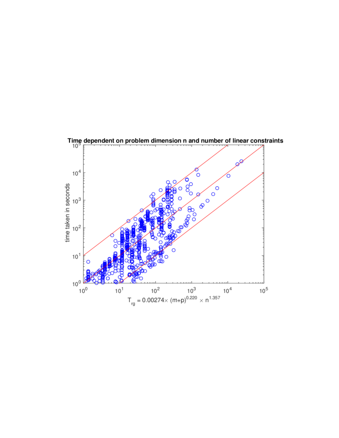
Figure 1: Time $T$ taken to solve 707 SDP instances versus the times estimated based on regression $T_{\rm rg}=0.00274\,(m+p)^{0.220}\,n^{1.357}$.

Table 5: Summary of numerical results obtained by Sdpnal$+$ in solving 707 SDP problems (each with the computation time of more than one second). In each cell, the first number is the number of problems solved, and the second number is the average time taken to solve the problems. Here $K$ means a thousand.

$m+p$	$\leq 1K$	$(1K,4K]$	$(4K,16K]$	$(16K,64K]$	$(64K,256K]$	$(256K,1024K]$	$>1024K$
$n\leq 100$	$\begin{array}[]{l}36\\ 2.04\end{array}$	$\begin{array}[]{l}16\\ 2.16\end{array}$	$\begin{array}[]{l}11\\ 8.74\end{array}$
$100<n\leq 200$	$\begin{array}[]{l}101\\ 6.29\end{array}$	$\begin{array}[]{l}4\\ 9.48\end{array}$	$\begin{array}[]{l}43\\ 25.67\end{array}$	$\begin{array}[]{l}43\\ 61.57\end{array}$
$200<n\leq 400$	$\begin{array}[]{l}127\\ 29.17\end{array}$	$\begin{array}[]{l}8\\ 14.07\end{array}$	$\begin{array}[]{l}15\\ 3.88\end{array}$	$\begin{array}[]{l}40\\ 95.25\end{array}$	$\begin{array}[]{l}20\\ 269.95\end{array}$
$400<n\leq 800$	$\begin{array}[]{l}44\\ 134.97\end{array}$	$\begin{array}[]{l}14\\ 603.19\end{array}$	$\begin{array}[]{l}8\\ 55.52\end{array}$	$\begin{array}[]{l}16\\ 34.75\end{array}$	$\begin{array}[]{l}14\\ 22.62\end{array}$	$\begin{array}[]{l}15\\ 2067.98\end{array}$
$800<n\leq 1600$	$\begin{array}[]{l}10\\ 168.62\end{array}$	$\begin{array}[]{l}56\\ 871.80\end{array}$	$\begin{array}[]{l}22\\ 496.73\end{array}$	$\begin{array}[]{l}7\\ 115.58\end{array}$	$\begin{array}[]{l}10\\ 250.14\end{array}$	$\begin{array}[]{l}5\\ 172.92\end{array}$
$1600<n\leq 3200$		$\begin{array}[]{l}1\\ 2672.64\end{array}$		$\begin{array}[]{l}8\\ 2867.77\end{array}$	$\begin{array}[]{l}1\\ 439.11\end{array}$	$\begin{array}[]{l}5\\ 2291.35\end{array}$	$\begin{array}[]{l}1\\ 966.32\end{array}$
$n>3200$			$\begin{array}[]{l}1\\ 12817.94\end{array}$				$\begin{array}[]{l}5\\ 11512.53\end{array}$

7 Conclusion and future works

Sdpnal$+$ is designed to be a general purpose software for solving large scale SDP problems with bound constraints as well as having a large number of equality and/or inequality constraints. The solver has been demonstrated to be fairly robust and highly efficient in solving various classes of SDP problems arising from the relaxation of combinatorial optimization problems such as maximum stable set problems, quadratic assignment problems, frequency assignment problems, binary quadratic integer programming problems. It has also worked well on SDP problems arising from the relaxation of robust clustering problems, rank-one tensor approximation problems, as well as problems arising from electronic structure calculations in quantum chemistry.

Our solver is expected to work well on nondegenerate well-posed SDP problems, but much more future work must be done to make the solver to work well on degenerate and/or ill-posed problems. Currently our solver is not catered to problems with SOCP or exponential cone constraints. As an obvious extension, we are currently extending the solver to handle problems with the aforementioned cone constraints.

We have also designed a basic user friendly interface for the user to input their SDP model into the solver. One of our future works is to expand the flexibility and capability of the interface such as the ability to handle Hermitian matrices.

References

- [1] S. Burer, R. D. Monteiro, and Y. Zhang, A computational study of a gradient-based log-barrier algorithm for a class of large-scale SDPs, Mathematical Programming, 95 (2003), pp. 359–379.
- [2] L. Chen, D. F. Sun, and K. C. Toh, An efficient inexact symmetric Gauss-Seidel based majorized ADMM for high-dimensional convex composite conic programming, Mathematical Programming, 161 (2017), pp. 237–270.
- [3] A. Eisenblätter, M. Grötschel, and A. M. Koster, Frequency planning and ramifications of coloring, Discussiones Mathematicae Graph Theory, 22 (2002), pp. 51–88.
- [4] M. Grant and S. Boyd, CVX: Matlab software for disciplined convex programming, version 2.1. http://cvxr.com/cvx, Mar. 2014.
- [5] P. Hahn and M. Anjos, QAPLIB – a quadratic assignment problem library. http://www.seas.upenn.edu/qaplib.
- [6] N.-H. Z. Leung and K. C. Toh, An SDP-based divide-and-conquer algorithm for large scale noisy anchor-free graph realization, SIAM J. Scientific Computing, 31 (2009), pp. 4351–4372.
- [7] X. D. Li, D. F. Sun, and K. C. Toh, A Schur complement based semi-proximal ADMM for convex quadratic conic programming and extensions, Mathematical Programming, 155 (2016), pp. 333–373.
- [8] L. Lovasz, On the shannon capacity of a graph, IEEE Transactions on Information Theory, 25 (1979), pp. 1–7.
- [9] J. Lfberg, Yalmip: A tool box for modeling and optimization in matlab, in 2004 IEEE International Symposium on Computer Aided Control Systems Design, 2004.
- [10] R. Monteiro, C. Ortiz, and B. Svaiter, A first-order block-decomposition method for solving two-easy-block structured semidefinite programs, Mathematical Programming Computation, (2013), pp. 1–48.
- [11] J. Nie and L. Wang, Semidefinite relaxations for best rank-1 tensor approximations, SIAM J. on Matrix Analysis and Applications, 35 (2014), pp. 1155–1179.
- [12] J. Peng and Y. Wei, Approximating k-means-type clustering via semidefinite programming, SIAM J. on Optimization, 18 (2007), pp. 186–205.
- [13] J. Povh and F. Rendl, Copositive and semidefinite relaxations of the quadratic assignment problem, Discrete Optimization, 6 (2009), pp. 231–241.
- [14] N. Sloane, Challenge problems: Independent sets in graphs. http://www.research.att.com/∼njas/doc/graphs.html, 2005.
- [15] J. F. Sturm, Using SeDuMi 1.02, a Matlab toolbox for optimization over symmetric cones, Optimization Methods and Software, 11 (1999), pp. 625–653.
- [16] D. F. Sun, K. C. Toh, and L. Q. Yang, A convergent 3-block semi-proximal alternating direction method of multipliers for conic programming with 4-type constraints, SIAM J. Optimization, 25 (2015), pp. 882–915.
- [17] K. C. Toh, Solving large scale semidefinite programs via an iterative solver on the augmented systems, SIAM J. Optimization, 14 (2004), pp. pp. 670–698.
- [18] K. C. Toh, M. J. Todd, and R. H. Tutuncu, SDPT3 — a Matlab software package for semidefinite programming, Optimization Methods and Software, 11 (1999), pp. 545–581.
- [19] M. Trick, V. Chvatal, B. Cook, D. Johnson, C. McGeoch, and R. Tarjan, The second DIMACS implementation challenge — NP hard problems: Maximum clique, graph coloring, and satisfiability. http://dimacs.rutgers.edu/Challenges/, 1992.
- [20] R. H. Tutuncu, K. C. Toh, and M. J. Todd, Solving semidefinite-quadratic-linear programs using SDPT3, Mathematical Programming, 95 (2003), pp. 189–217.
- [21] Z. Wen, D. Goldfarb, and W. Yin, Alternating direction augmented Lagrangian methods for semidefinite programming, Mathematical Programming Computation, 2 (2010), pp. 203–230.
- [22] A. Wiegele, Biq mac library. http://biqmac.uni-klu.ac.at/biqmaclib.html, 2007.
- [23] M. Yamashita, K. Fujisawa, and M. Kojima, Implementation and evaluation of SDPA 6.0 (semidefinite programming algorithm 6.0), Optimization Methods and Software, 18 (2003), pp. 491–505.
- [24] L. Q. Yang, D. F. Sun, and K. C. Toh, SDPNAL+: a majorized semismooth Newton-CG augmented Lagrangian method for semidefinite programming with nonnegative constraints, Mathematical Programming Computation, 7 (2015), pp. 331–366.
- [25] X.-Y. Zhao, D. F. Sun, and K. C. Toh, A Newton-CG augmented Lagrangian method for semidefinite programming, SIAM J. Optim., 20 (2010), pp. 1737–1765.