Inferring energy dissipation from violation of the Fluctuation-Dissipation Theorem

Abstract

The Harada-Sasa equality elegantly connects the energy dissipation rate of a moving object with its measurable violation of the Fluctuation-Dissipation Theorem (FDT). Although proven for Langevin processes, its validity remains unclear for discrete Markov systems whose forward and backward transition rates respond asymmetrically to external perturbation. A typical example is a motor protein called kinesin. Here we show generally that the FDT violation persists surprisingly in the high-frequency limit due to the asymmetry, resulting in a divergent FDT violation integral and thus a complete breakdown of the Harada-Sasa equality. A renormalized FDT violation integral still well predicts the dissipation rate when each discrete transition produces a small entropy in the environment. Our study also suggests a new way to infer this perturbation asymmetry based on the measurable high-frequency-limit FDT violation.

Introduction.–Recent development of technology has allowed direct observation and control of molecular fluctuations, thus opening up a new field to explore nano machines that operate out of equilibrium toyabe2015nonequilibrium ; martinez2017colloidal ; ciliberto2017experiments . An important approach to investigate a stochastic system is to study both its spontaneous fluctuation and the elicited response to perturbation. For the recorded velocity $\dot{x}_{t}$ of a particle (with $x_{t}$ being its position at time $t$), its spontaneous fluctuation is captured by the temporal correlation function: $C_{\dot{x}}(t-\tau)\equiv\langle(\dot{x}_{t}-\langle\dot{x}\rangle_{ss})(\dot{x}_{\tau}-\langle\dot{x}\rangle_{ss})\rangle_{ss}$, with $\langle\cdot\rangle_{ss}$ denoting the average over the stationary ensemble. On the other hand, the velocity response to a small external force $h$ is captured by the temporal response function determined from the functional derivative $R_{\dot{x}}(t-\tau)\equiv\delta\langle\dot{x}_{t}\rangle/\delta h_{\tau}$. For equilibrium systems, these two functions are closely related through the fundamental Fluctuation-Dissipation Theorem (FDT) kubo1966fluctuation , which in the Fourier space reads

$$\tilde{C}_{\dot{x}}(\omega)=2Tk_{B}\tilde{R}_{\dot{x}}^{\prime}(\omega),$$ (1)

where prime denotes the real part, $T$ is the bath temperature, and the Boltzmann factor $k_{B}$ is set to be 1 hereafter. Violation of the FDT has been widely used to characterize non-equilibrium systems, including glassy systems cugliandolo1997fluctuation ; LeticiaPREtemperature , hair bundles martin2001comparison , and cytoskeleton networks Mizuno2007cytoskeletonNetwork .

The generalization of the FDT for systems in non-equilibrium steady state has been studied intensively baiesi2009fluctuations ; seifert2010fluctuation ; baiesi2013update ; speck2006restoring ; prost2009generalized . In particular, for systems described by Langevin equations, Harada and Sasa have shown that the violation integral of the FDT gives the dissipation rate $\dot{q}$ for the observed variable $x$ harada2005equality ; harada2006energy ; harada2007fluctuations :

$$I\equiv\langle\dot{x}\rangle_{ss}^{2}+\int_{-\infty}^{\infty}\Big{[}\tilde{C}_{\dot{x}}(\omega)-2T\tilde{R}_{\dot{x}}^{\prime}(\omega)\Big{]}\frac{d\omega}{2\pi}=\frac{\dot{q}}{\gamma},$$ (2)

with $\gamma$ the friction coefficient. The Harada-Sasa (HS) equality has been applied successfully to infer the energetics of F1-ATPase, a rotary motor protein toyabe2015single ; toyabe2010nonequilibrium . Our recent study demonstrated that it is also useful for inferring hidden dissipation of timescale-separated systems when having access to only slow variables Wang2016entropy ; Wang2016FRRviolation . Eq. (2) has also been generalized to more elaborated Langevin systems DeutschNarayan2006 ; fodor2016far ; nardini2017entropy .

Although the HS equality seems very general, its validity remains unclear for discrete Markov processes. In this context, Lippiello et al. have shown that the HS equality is recovered when entropy production in the environment is small for each jump Lippiello2014fluctuation . A central assumption there is that the forward and backward transition rates respond symmetrically to the external perturbation. However, this symmetry is violated for molecular motors, according to recent experimental and modeling work zimmermann2012efficiencies ; kawaguchi2014nonequilibrium ; Zimmermann2015motors ; brown2017allocating ; taniguchi2005entropy ; ariga2017nonequilibrium . Furthermore, various forms of generalized FDT that go beyond symmetric perturbation reveal non-trivial dependence on the asymmetry diezemann2005fluctuation ; maes2010response ; seifert2010fluctuation , in sharp contrast with the simplicity of the HS equality.

Here, we clarify the connection between dissipation rate and violation of the FDT for Markov systems with perturbation asymmetry. We find surprisingly that the FDT is violated even in the high-frequency limit, leading to a divergent FDT violation integral, although the dissipation rate remains finite. We propose two renormalization schemes to remove the divergence of the FDT violation integral, and show that the renormalized integrals well predict the dissipation rate when the entropic change per jump is small. The main results are illustrated with a minimum model for kinesin.

General Markov systems.–Consider a general Markov process with $N$ states. The transition from state $n$ to state $m$ ($1\leq n,m\leq N$) happens with rate $w_{n}^{m}$. The probability $P_{n}(t)$ at state $n$ and time $t$ evolves according to the following master equation

$$\frac{d}{dt}P_{n}(t)=\sum_{m}M_{nm}P_{m}(t),$$ (3)

where $M$ is assumed to be an irreducible transition rate matrix determined by $M_{nm}=w_{m}^{n}-\delta_{nm}\sum_{k}w_{n}^{k}$, with $\delta_{nm}$ being the Kronecker delta. The $j$-th left and right eigenmodes, denoted as $x_{j}(n)$ and $y_{j}(n)$ respectively, satisfy the characteristic equations $\sum_{m}M_{nm}x_{j}(m)=-\lambda_{j}x_{j}(n)$ and $\sum_{m}y_{j}(m)M_{mn}=-\lambda_{j}y_{j}(n)$. Here, the minus sign is introduced to have an “eigenvalue” $\lambda_{j}$ with a positive real component van1992stochastic . These eigenvalues are arranged in the ascending order by their real part, i.e., $\text{Re}(\lambda_{1})\leq\text{Re}(\lambda_{2})\leq\cdots$. This system has a unique stationary distribution $P_{m}^{ss}$ that satisfies $\sum_{m}P_{m}^{ss}=1$. For the ground state associated with $\lambda_{1}=0$, $y_{1}(n)$ should be constant and $x_{1}(m)$ be proportional to $P_{m}^{ss}$. Here, we fix $y_{1}=1$ and $x_{1}(m)=P_{m}^{ss}$. For this system, we can always find a set of eigenmodes that satisfy the orthogonal relations $\sum_{m}x_{j}(m)y_{j^{\prime}}(m)=\delta_{jj^{\prime}}$ and completeness relations $\sum_{j}x_{j}(n)y_{j}(m)=\delta_{nm}$, which we use in the following analysis. The left and right eigenmodes are coupled for equilibrium systems: $x_{j}(m)=y_{j}(m)P_{m}^{eq}$. This is not true for non-equilibrium systems.

We introduce an external perturbation $h$ that modifies the transition rates to be

$$\tilde{w}_{m}^{n}=w_{m}^{n}\exp\left[h(\theta_{n}^{m}+\frac{1}{2})\frac{\mathcal{Q}_{n}-\mathcal{Q}_{m}}{T}\right].$$ (4)

Here, $\mathcal{Q}_{m}$ is a variable conjugate to perturbation $h$, and $\theta_{n}^{m}$ parameterizes the asymmetry of the transition rates in response to external perturbation. $\theta_{n}^{m}$ may vary for different transitions, but should satisfy $\theta_{n}^{m}=-\theta_{m}^{n}$. $\theta_{n}^{m}=0$ corresponds to the symmetric case. We are interested in the correlation and response spectrum of the velocity observable $\dot{Q}_{t}=d\mathcal{Q}_{n_{t}}/dt$. The strategy is to project these spectra onto the eigenspace. We introduce the projection coefficients: $\alpha_{j}\equiv\sum_{n}\mathcal{Q}_{n}x_{j}(n)$, $\beta_{j}\equiv\sum_{n}\mathcal{Q}_{n}y_{j}(n)P_{n}^{ss}$, and $\phi_{j}\equiv\sum_{n}B_{n}y_{j}(n)$, where $B_{n}$ captures the effect from perturbation, and is given by $B_{n}=\sum_{m}(\theta_{n}^{m}J_{n}^{m}+\mathcal{A}_{n}^{m})(\mathcal{Q}_{n}-\mathcal{Q}_{m})/T$. Here, $\mathcal{A}_{n}^{m}\equiv(w_{n}^{m}P_{n}^{ss}+w_{m}^{n}P_{m}^{ss})/2$ is the dynamical activity between state $n$ and $m$, while $J_{n}^{m}\equiv w_{n}^{m}P_{n}^{ss}-w_{m}^{n}P_{m}^{ss}$ is the net flux from state $n$ to $m$. Then, we obtain

$$\tilde{C}_{\dot{Q}}(\omega) = \sum_{j=2}^{N}2\alpha_{j}\beta_{j}\lambda_{j}\Big{[}1-\frac{1}{1+(\omega/\lambda_{j})^{2}}\Big{]},$$ (5a)

$$\tilde{R}_{\dot{Q}}(\omega) = \sum_{j=2}^{N}\alpha_{j}\phi_{j}\Big{[}1-\frac{1+i(\omega/\lambda_{j})}{1+(\omega/\lambda_{j})^{2}}\Big{]},$$ (5b)

with $i$ the imaginary unit. We have used this framework previous in the context of symmetric perturbation Wang2016entropy ; Wang2016FRRviolation . See Supplemental Material supp for more details.

Let us consider the high frequency limit first. According to Eq. (5), we have $\tilde{C}_{\dot{Q}}(\infty)=\sum_{j=2}^{N}2\alpha_{j}\beta_{j}\lambda_{j}$ and $\tilde{R}_{\dot{Q}}(\infty)=\sum_{j=2}^{N}\alpha_{j}\phi_{j}$. Following the definitions of these coefficients, we obtain

$$\tilde{C}_{\dot{Q}}(\infty) = \sum_{n,m}(\mathcal{Q}_{n}-\mathcal{Q}_{m})^{2}\mathcal{A}_{n}^{m},$$ (6a)

$$\tilde{R}_{\dot{Q}}(\infty) = \frac{1}{2T}\sum_{n,m}(\mathcal{Q}_{n}-\mathcal{Q}_{m})^{2}\Big{(}\theta_{n}^{m}J_{n}^{m}+\mathcal{A}_{n}^{m}\Big{)}.\quad$$ (6b)

In obtaining Eq. (6a), we note that $\sum_{j}x_{j}(n)\lambda_{j}y_{j}(m)=-M_{nm}$, and that any summation over the full state space is invariant under the switching of the label, i.e., $n\leftrightarrow m$. Because $\theta$ is introduced only at the stage of perturbation here, the correlation spectrum does not depend on $\theta$. More specifically, $\tilde{C}_{\dot{Q}}(\infty)$ only depends on the activity $\mathcal{A}_{n}^{m}$, while $\tilde{R}_{\dot{Q}}(\infty)$ has an additional dependence on the flux $J_{n}^{m}$ in the presence of an asymmetric load-sharing factor. The FDT violation in the high-frequency limit is then

$$\mathcal{V}_{\infty}\equiv\lim_{\omega\to\infty}\Big{[}\tilde{C}_{\dot{x}}(\omega)-2T\tilde{R}_{\dot{x}}^{\prime}(\omega)\Big{]}=-\sum_{n,m}\theta_{m}^{n}J_{m}^{n}(\mathcal{Q}_{m}-\mathcal{Q}_{n})^{2}.$$ (7)

It vanishes for any equilibrium systems ($J_{m}^{n}=0$) or non-equilibrium systems with symmetric perturbation ($\theta_{m}^{n}=0$). Otherwise, a finite FDT violation persists even in the high-frequency limit, which is quite surprising. When the transitions are dominated by futile back-and-forth jumps, i.e., $|\mathcal{A}_{n}^{m}|\gg|J_{n}^{m}|$, the system has a relatively small high-frequency-limit violation, i.e., $|\mathcal{V}_{\infty}/\tilde{C}_{\dot{Q}}(\infty)|\ll 1$. This will be the typical case when individual jumps produce a small entropic change in the environment, as will be illustrated later.

The direct consequence of a non-zero $\mathcal{V}_{\infty}$ is a divergent FDT violation integral $I$ and thus complete breakdown of the HS equality (as the dissipation rate still remains finite). To get rid of divergence, we first subtract $\mathcal{V}_{\infty}$ from the violation spectrum and then introduce the renormalized FDT violation integral:

$$I_{*}\equiv\langle\dot{Q}\rangle_{ss}+\int_{-\infty}^{\infty}\Big{[}\tilde{C}_{\dot{Q}}(\omega)-2T\tilde{R}^{\prime}_{\dot{Q}}(\omega)-\mathcal{V}_{\infty}\Big{]}\frac{d\omega}{2\pi}.$$ (8)

A more practical scheme of renormalization will be discussed towards the end. Combined with Eq. (5), we obtain $I_{*}=\sum_{j}\lambda_{j}\alpha_{j}\left(T\phi_{j}-\beta_{j}\lambda_{j}\right)$ note . Using the definitions of these coefficients and summing over all eigenmodes, we obtain supp

$$I_{*}=\sum_{n,m}\Big{(}\frac{\bar{\nu}_{n}+\bar{\nu}_{m}}{4}+\frac{\bar{\nu}_{n}-\bar{\nu}_{m}}{2}\theta_{n}^{m}\Big{)}J_{n}^{m}(\mathcal{Q}_{m}-\mathcal{Q}_{n}),$$ (9)

where $\bar{\nu}_{n}\equiv\sum_{m}w_{n}^{m}(\mathcal{Q}_{m}-\mathcal{Q}_{n})$ is the average change rate of $Q_{t}$ when it starts from state $n$. Evidently from this equation, the FDT violation only comes from transitions that change the observable $\mathcal{Q}_{n}$, as it should, and it is proportional to the local net flux $J_{n}^{m}$, the signature of non-equilibrium systems. Below, we discuss the structure of $\mathcal{V}_{\infty}$ and the connection between $I_{*}$ and the dissipation rate through more specific models.

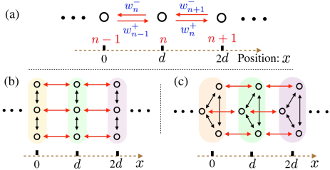
Figure 1: (a) One-dimensional (1-d) hopping process. (b)(c) Multi-dimensional hopping models. The corresponding observable $\mathcal{Q}_{n}$, which is $x$ here, does not distinguish microscopic states within each colored block. As with the 1-d hopping model, we assume that $\theta$ is the same for all red transitions. These models may describe molecular motors that hop along a discrete lattice with several internal chemical states. They also resemble sensory adaptation model in E.coli shouwen2015adaptation .

Application to various models.– Consider a particle hopping along a discrete lattice with a lattice constant $d$, as illustrated in FIG. 1(a). Each state $n$ has a well-defined energy $U_{n}$. The transition rates are assumed to satisfy

$$w_{n}^{+} = w_{0}\exp\Big{(}(\theta+\frac{1}{2})\frac{\Delta U_{n}+hd}{T}\Big{)},$$ (10a)

$$w_{n+1}^{-} = w_{0}\exp\Big{(}(\theta-\frac{1}{2})\frac{\Delta U_{n}+hd}{T}\Big{)},$$ (10b)

with $w_{0}$ the constant prefactor, and $\Delta U_{n}\equiv U_{n}-U_{n+1}$ the dissipation per jump. This model satisfies local detailed balance, i.e., $w_{n}^{+}/w_{n+1}^{-}=\exp([\Delta U_{n}+hd]/T)$. We assume that $U_{n}$ is constructed from a continuous function $U(x)$ via $U_{n}=U(nd)$. The energy landscape can be tilted to drive the system out of equilibrium.

Firstly, we derive the high-frequency violation $\mathcal{V}_{\infty}$. For this system, the conjugate observable $\mathcal{Q}_{n}$ is position $x$. We note that $(\mathcal{Q}_{m}-\mathcal{Q}_{n})^{2}=d^{2}$ for all allowed transitions. Furthermore, both the flux $J=\langle\dot{x}\rangle_{ss}/L$ and the asymmetric factor $\theta$ are constant in the state space. Therefore, Eq. (7) is reduced to

$$\mathcal{V}_{\infty}=-2\theta\langle\dot{x}\rangle_{ss}d.$$ (11)

This simple relation (11) can be easily generalized to multi-dimensional hopping processes illustrated in Fig. 1(b)(c), by lumping states within each colored block and fluxes between two connected blocks. For such multi-dimensional models, $\mathcal{V}_{\infty}$ may vanish even if the system remains out of equilibrium, as $\langle\dot{x}\rangle_{ss}=0$ is not a sufficient condition for equilibrium here. This is not possible for 1-d systems.

Secondly, we derive the renormalized HS equality. According to $I_{*}$ in Eq. (9), we have

$$I_{*}=d\sum_{n}\Big{(}\frac{\bar{\nu}_{n}+\bar{\nu}_{n+1}}{2}+\theta(\bar{\nu}_{n}-\bar{\nu}_{n+1})\Big{)}J_{n}^{n+1}.$$ (12)

Here, $\bar{\nu}_{n}=d(w_{n}^{+}-w_{n}^{-})$. We introduce $\epsilon_{n}\equiv\ln[w_{n}^{+}/w_{n+1}^{-}]$ as the entropy produced in the environment per jump, which has a characteristic amplitude $\epsilon$. Expanding Eq. (12) in Taylor series of $\epsilon$, we have $\bar{\nu}_{n}+\bar{\nu}_{n+1}=2w_{0}d\epsilon_{n}+\theta O(\epsilon^{2})+O(\epsilon^{3})$ and $\bar{\nu}_{n}-\bar{\nu}_{n+1}=O(\epsilon^{2})$ supp , which gives

$$I_{*}=w_{0}d^{2}\sum_{n}J_{n}^{n+1}\epsilon_{n}\Big{(}1+\theta O(\epsilon)+O(\epsilon^{2})\Big{)}.$$ (13)

We identify $\dot{q}=T\sum_{n}J_{n}^{n+1}\epsilon_{n}$ as the dissipation rate of the stochastic trajectory $Q_{t}$, and $\gamma_{*}=T/(w_{0}d^{2})$ as the effective friction coefficient. Finally, we obtain

$$\gamma_{*}I_{*}=\dot{q}\Big{(}1+\theta O(\epsilon)+O(\epsilon^{2})\Big{)}.$$ (14)

The renormalized HS equality, i.e., $\gamma_{*}I_{*}=\dot{q}$, is recovered when $\epsilon$ is small, regardless of asymmetry and discreteness. While the asymmetry leads to a first order deviation, the deviation of discreteness is only of the second order, thus much smaller. The assumption of a constant $\theta$ is crucial here. Throughout the derivation, we did not assume that $J_{n}^{n+1}$ is constant, a characteristic property of 1-d systems. Hence, Eq. (14) can be generalized to multi-dimensional models in Fig. 1(b)(c), as discussed in Supplemental Material supp .

Minimum model for kinesin.–A kinesin is a type of molecular motor that, powered by ATP, moves along microtubule filaments. Following the experimental and modeling work in taniguchi2005entropy , we use the biased diffusive model presented in Fig. 2(a) to describe the stepwise dynamics of this motor, with $d$ the step size. This is a special case of the 1-d hopping model that has translational invariance. The dissipation per jump $\Delta U$ can be tuned by changing ATP concentration, and $h$ is the external force that is applied to the bead attached to the motor in a typical experimental setup. Experiments show that the external force only affects the forward transition rate $w_{+}$ taniguchi2005entropy , as illustrated in Fig. 2(b). This situation occurs when the external force only varies the energy barrier for the forward transition (Fig. 2c). The scenario of kinesin corresponds to a completely asymmetric model with $\theta=0.5$.

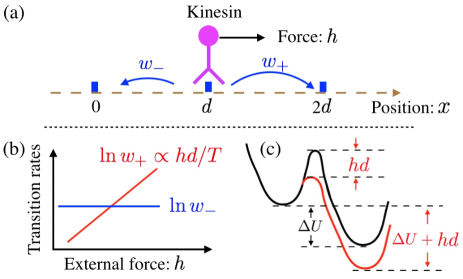
Figure 2: (a) A simplified Markov model for kinesin. (b) The experimentally suggested relations between transition rates $w_{\pm}$ and the external force $h$ taniguchi2005entropy , corresponding to the case with $\theta=0.5$. (c) The energy landscape connecting neighboring states. The external force only varies the energy barrier for the forward transition.

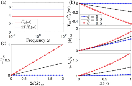
Figure 3: (a) The correlation spectrum $\tilde{C}_{\dot{x}}(\omega)$ and the (real part of) response spectrum $\tilde{R}_{\dot{x}}^{\prime}(\omega)$ for the velocity $\dot{x}_{t}$, obtained at $\Delta U=1$ and $\theta=0.5$. A finite violation of FDT, $\mathcal{V}_{\infty}$, persists even in the high frequency limit. (b) The relative violation of the FDT in the high-frequency limit [$\mathcal{V}_{\infty}/\tilde{C}_{\dot{x}}(\infty)$], the average drifting velocity $\langle\dot{x}\rangle_{ss}$, and the predicted dissipation rate $\gamma_{*}I_{*}$ based on the renormalized FDT violation integral against the actual rate $\dot{q}$. Here, the control parameter is the entropic change per jump, i.e., $\Delta U/T$. (c) Verification of Eq. (11). The slope of each curve gives the corresponding $\theta$. Other parameters: $w_{0}=1$, $d=1$, and $h=0$.

This simple model allows analytical solutions. At the steady state with $h=0$, the average velocity is given by $\langle\dot{x}\rangle_{ss}=d(w_{+}-w_{-})$, and the dissipation rate $\dot{q}=\Delta U\langle\dot{x}\rangle_{ss}/d=\Delta U(w_{+}-w_{-})$. The correlation spectrum of the velocity $\dot{x}$ is found to be $\tilde{C}_{\dot{x}}(\omega)=(\omega_{+}+\omega_{-})d^{2}$, while the response spectrum of the velocity, measured via applying a small and periodic force, is given by $\tilde{R}_{\dot{x}}(\omega)=d^{2}[2\theta(w_{+}-w_{-})+(w_{+}+w_{-})]/2T$. These spectra are constant in the frequency domain due to the translational invariance of this simple model. Indeed, the FDT is violated even in the high frequency limit due to the presence of asymmetry, as illustrated in Fig. 3(a).

The relative high-frequency violation $\mathcal{V}_{\infty}/\tilde{C}_{\dot{x}}(\infty)$ becomes smaller when the entropic change per transition, i.e., $\Delta U/T$, decreases [Fig. 3(b)]. It can be checked easily that Eq. (11) holds here, as illustrated in Fig. 3(c). Therefore, a smaller driving energy $\Delta U$ reduces $\mathcal{V}_{\infty}$ by slowing down the biased motion [Fig. 3(b)]. Such a violation has been noticed recently in a more realistic model of kinesin ariga2017nonequilibrium . For a small $\Delta U/T$, the renormalized FDT violation integral $I_{*}$ multiplied with the effective friction $\gamma_{*}$ well predicts the dissipation rate $\dot{q}$, as shown in Fig. 3(b).

Practical renormalization.– An important parameter in applying the HS equality is the ambient temperature $T$, which is very challenging to determine (or control) experimentally due to the tiny size of the molecular machine. In practice, $T$ has been determined from the ratio $\tilde{C}_{\dot{x}}(\omega)/2\tilde{R}_{\dot{x}}^{\prime}(\omega)$ in the high-frequency regime, assuming that FDT is satisfied there toyabe2010nonequilibrium ; toyabe2015single ; ariga2017nonequilibrium . According to our current study, this assumption might be wrong in the presence of perturbation asymmetry. In fact, the high-frequency violation leads to a modified temperature:

$$T_{re}\equiv\lim_{\omega\to\infty}\frac{\tilde{C}_{\dot{x}}(\omega)}{2\tilde{R}_{\dot{x}}^{\prime}(\omega)}=\frac{T}{1-\mathcal{V}_{\infty}/\tilde{C}_{\dot{x}}(\infty)}.$$ (15)

It is reduced to the bath temperature when $\mathcal{V}_{\infty}=0$. With this temperature, we obtain a renormalized FDT violation integral that becomes well-behaved:

$$I_{re}\equiv\langle\dot{x}\rangle_{ss}^{2}+\int_{-\infty}^{\infty}\Big{[}\tilde{C}_{\dot{x}}(\omega)-2T_{re}\tilde{R}_{\dot{x}}^{\prime}(\omega)\Big{]}\frac{d\omega}{2\pi}.$$ (16)

The effective friction coefficient $\gamma_{re}$ can be determined from

$$\gamma_{re}\equiv\lim_{\omega\to\infty}\frac{1}{\tilde{R}_{\dot{x}}^{\prime}(\omega)},$$ (17)

which is an exact relation for Langevin systems, and serves as a generalization here. When the entropic change per jump is small, we have $\mathcal{V}_{\infty}/\tilde{C}_{\dot{x}}(\infty)\ll 1$, thus $I_{re}\approx I_{*}$ and $\gamma_{re}\approx\gamma_{*}$. Therefore, $\gamma_{re}I_{re}$ also becomes a reasonable estimation of the dissipation rate $\dot{q}$ when the entropic change per jump is small. This is illustrated numerically in Supplemental Material using the 1-d hopping model supp . When the high-frequency FDT violation is relatively small, different renormalization schemes converge to the same correct answer, although the original HS equality still breaks down due to the divergence of the FDT violation integral $I$.

Conclusion.–We have demonstrated for Markov systems that the FDT violation persists generally in the high frequency limit in the presence of asymmetric perturbation. This is in sharp contrast to our physical intuition that the high-frequency correlation and response essentially reflect only the thermal property of the bath. The high-frequency violation leads to a divergent FDT violation integral that invalidates the HS equality. However, proper renormalization of the FDT violation integral restores the HS equality effectively when the entropic change in the environment is small for each jump. Hence, our study provides a protocol to estimate the dissipation rate for discrete Markov systems with asymmetry, based on the measured correlation and response spectra. Our study also reveals a linear relation between the high-frequency-limit violation and the asymmetric factor $\theta$, and therefore can be exploited to infer $\theta$ experimentally. We believe that our results will guide further investigation of kinesin ariga2017nonequilibrium .

Supplemental Material

.1 Correlation, response, and FDT violation in general Markov models

.1.1 Correlation spectrum

Noting that the correlation function for $Q_{t}$ satisfies $C_{Q}(t-\tau)\equiv\langle[Q_{t}-\langle Q\rangle_{ss}][Q_{\tau}-\langle Q\rangle_{ss}]\rangle_{ss}$, we have

$$C_{\dot{Q}}(t-\tau)=\frac{\partial^{2}C_{Q}(t-\tau)}{\partial\tau\partial t}.$$ (S1)

It is easier to calculate $C_{Q}(t-\tau)$ first. Assuming $t\geq\tau$, it satisfies

$$C_{Q}(t-\tau)=\sum_{n,n^{\prime}}\mathcal{Q}_{n}\mathcal{Q}_{n^{\prime}}P(t-\tau;n,n^{\prime})P_{n^{\prime}}^{ss}-\langle Q\rangle_{ss}^{2},$$ (S2)

where $P(t-\tau;n,n^{\prime})$ is the propagator, or the probability for reaching state $n$ at time $t$, assuming that the system starts from state $n^{\prime}$ at time $\tau$. In the eigenspace,

$$P(t-\tau;n,n^{\prime})=\sum_{j}y_{j}(n^{\prime})e^{-\lambda_{j}|t-\tau|}x_{j}(n).$$ (S3)

Indeed, it is the solution of the corresponding master equation (3) in the Main Text, given the initial condition $P(0;n,n^{\prime})=\delta_{nn^{\prime}}$. Inserting this relation back to Eq. (S2) and introducing the projection of $\mathcal{Q}$ on the $j$-th eigenmode, i.e., $\alpha_{j}\equiv\sum_{n}\mathcal{Q}_{n}x_{j}(n)$ and $\beta_{j}\equiv\sum_{n}\mathcal{Q}_{n}y_{j}(n)P_{n}^{ss}$, we obtain the expansion of correlation function in the eigenspace:

$$C_{Q}(t-\tau)=\sum_{j=2}^{N}\alpha_{j}\beta_{j}e^{-\lambda_{j}|t-\tau|}.$$ (S4)

The contribution of the first eigenmode is counteracted by $\langle Q\rangle^{2}_{ss}$. Stationarity of the system guarantees that $C_{Q}(t-\tau)=C_{Q}(\tau-t)$. Therefore, Eq. (S4) obtained from $t\geq\tau$ is also applicable for $t<\tau$. We use the following convention for Fourier transform:

$$\tilde{f}(\omega)=\int_{-\infty}^{\infty}f(t)\exp(i\omega t)dt,\quad f(t)=\int_{-\infty}^{\infty}\tilde{f}(\omega)\exp(-i\omega t)\frac{d\omega}{2\pi}.$$ (S5)

Combining Eq. (S1), Fourier transformation and Eq. (S4), we finally obtain the velocity correlation spectrum (6a) in the Main Text.

.1.2 Response spectrum

The response spectrum can be obtained by studying the response of the system to a periodic perturbation. Consider $h_{t}=h_{0}\exp(-i\omega t)$ with $h_{0}$ a small amplitude and $i$ the imaginary unit. Expanded in Taylor series, the modified transition rate matrix $\tilde{M}$ is given by

$$\tilde{M}=M+M^{*}h_{0}\exp(-i\omega t)+O(h_{0}^{2}),$$ (S6)

where $M^{*}\equiv\partial_{h}\tilde{M}|_{h\to 0}$. On the other hand, the modified distribution can also be expanded up to the first order:

$$\tilde{P}_{m}=P_{m}^{ss}+P^{*}_{m}h_{0}\exp(-i\omega t)+O(h_{0}^{2}),$$ (S7)

with $P_{m}^{*}\equiv\partial_{h}\tilde{P}_{m}|_{h\to 0}$. Since $d\tilde{P}_{m}/dt=\sum_{n}\tilde{M}_{mn}\tilde{P}_{n}$ and $\sum_{n}M_{mn}P_{n}^{ss}=0$, we obtain in a Matrix form

$$P^{*}=-\frac{1}{M+i\omega}M^{*}P^{ss}.$$ (S8)

For the observable $Q_{t}$, its response spectrum is given by

$$\tilde{R}_{Q}(\omega)=\sum_{n}\mathcal{Q}_{n}P^{*}_{n}=\sum_{j=2}^{N}\frac{\alpha_{j}\phi_{j}}{\lambda_{j}-i\omega},$$ (S9)

where $\phi_{j}\equiv\sum_{n}B_{n}y_{j}(n)$ with $B_{n}\equiv\sum_{m}M^{*}_{nm}P^{ss}_{m}$. By using the transformation $R_{\dot{Q}}(t)=dR_{Q}/dt$ or $\tilde{R}_{\dot{Q}}(\omega)=-i\omega\tilde{R}_{Q}(\omega)$, we obtain the velocity response spectrum (6b) in the Main Text.

.1.3 The renormalized FDT violation integral $I_{*}$

We derive Eq. (9) in the Main Text. Firstly, note that $(T\phi_{j}-\lambda_{j}\beta_{j})$ is a key quantity in the violation spectrum integral:

$$I_{*}=\sum_{j}\lambda_{j}\alpha_{j}\left(T\phi_{j}-\beta_{j}\lambda_{j}\right).$$

According to definitions of these coefficients, we obtain

$$T\phi_{j}-\lambda_{j}\beta_{j}=\sum_{n,m}y_{j}(n)J_{m}^{n}\Big{(}\frac{\mathcal{Q}_{n}+\mathcal{Q}_{m}}{2}+\theta_{n}^{m}(\mathcal{Q}_{m}-\mathcal{Q}_{n})\Big{)}.$$

For equilibrium systems, the flux $J_{m}^{n}$ vanishes due to detailed balance. This leads to $T\phi_{j}=\beta_{j}\lambda_{j}$ for all eigenmodes, and thus the vanishing of the FDT violation integral. On the other hand, $\lambda_{j}\alpha_{j}=-\sum_{n}\bar{\nu}_{n}x_{j}(n)$, with $\bar{\nu}_{n}\equiv\sum_{m}w_{n}^{m}(\mathcal{Q}_{m}-\mathcal{Q}_{n})$ being the average change rate of $Q_{t}$ when it starts from state $n$. Combining these relations, we obtain the analytical expression for the effective FDT violation integral:

$$I_{*}=\sum_{n,m}\bar{\nu}_{n}J_{n}^{m}\Big{(}\frac{\mathcal{Q}_{n}+\mathcal{Q}_{m}}{2}+\theta_{n}^{m}(\mathcal{Q}_{m}-\mathcal{Q}_{n})\Big{)}.$$ (S10)

Noting that $\sum_{m}J_{n}^{m}=0$ due to stationarity, we can subtract $\sum_{n,m}\bar{\nu}_{n}J_{n}^{m}\mathcal{Q}_{n}$ (which is also zero) from $I_{*}$, and symmetrize the resulting expression to obtain Eq. (9) in the Main Text.

.2 The renormalized HS equality

Here, we provide more details of deriving the renormalized HS equality, give numerical illustrations, and present the generalization to higher dimensional models mentioned in the Main Text. First, we consider the 1-d hopping model mentioned in Fig. 1(a). Following Eq. (12), we are interested in how $\bar{\nu}_{n}+\bar{\nu}_{n+1}$ and $\bar{\nu}_{n}-\bar{\nu}_{n+1}$ behave when $\epsilon_{n}$ is small. Here, $\bar{\nu}_{n}=d(w_{n}^{+}-w_{n}^{-})$. More explicitly, we have

$$\begin{split}\bar{\nu}_{n}+\bar{\nu}_{n+1}&=w_{0}d\Big{[}(e^{(\theta+1/2)\epsilon_{n}}-e^{(\theta-1/2)\epsilon_{n-1}})+(e^{(\theta+1/2)\epsilon_{n+1}}-e^{(\theta-1/2)\epsilon_{n}})\Big{]}.\end{split}$$

Applying Taylor expansion, we obtain

$$\begin{split}\bar{\nu}_{n}+\bar{\nu}_{n+1}&=w_{0}d\Big{[}\epsilon_{n}+\frac{\epsilon_{n-1}+\epsilon_{n+1}}{2}+\theta(\epsilon_{n+1}-\epsilon_{n-1})\\ &+\theta(\epsilon_{n}^{2}+\frac{\epsilon_{n+1}^{2}+\epsilon_{n-1}^{2}}{2})+(\frac{1}{8}+\frac{1}{2}\theta^{2})(\epsilon_{n+1}^{2}-\epsilon_{n-1}^{2})+O(\epsilon^{3})\Big{]},\end{split}$$

with $\epsilon$ capturing the overall amplitude of $\epsilon_{n}$. Similarly, we have

$$\begin{split}\bar{\nu}_{n}-\bar{\nu}_{n+1}&=w_{0}d\Big{[}\frac{\epsilon_{n-1}-\epsilon_{n+1}}{2}+2\theta(\epsilon_{n}-\frac{\epsilon_{n+1}+\epsilon_{n-1}}{2})\\ &+(\frac{1}{4}+\theta^{2})(\epsilon_{n}^{2}-\frac{\epsilon_{n-1}^{2}+\epsilon_{n+1}^{2}}{2})-\frac{\theta}{2}(\epsilon_{n+1}^{2}-\epsilon_{n-1}^{2})+O(\epsilon^{3})\Big{]}.\end{split}$$

Now, we assume $\epsilon_{n}=\epsilon f(nd)$, with $f(x)$ a continuous function and $\epsilon\propto d$. The motivation of this assumption is that there is an underlying smooth energy landscape, as discussed in the Main Text. From Taylor expansion, we obtain

$$\epsilon_{n\pm 1}=\epsilon\Big{[}f(nd)\pm\frac{\partial f}{\partial x}d+\frac{1}{2}\frac{\partial^{2}f}{\partial x^{2}}d^{2}+O(\frac{d^{3}}{L^{3}})\Big{]}.$$

Therefore, we have

$$\epsilon_{n+1}+\epsilon_{n-1} = 2\epsilon_{n}+O\Big{(}\epsilon\frac{d^{2}}{L^{2}}\Big{)},$$ (S11)

$$\epsilon_{n+1}-\epsilon_{n-1} = 2\epsilon\frac{\partial f}{\partial x}d+O\Big{(}\epsilon\frac{d^{3}}{L^{3}}\Big{)},$$ (S12)

$$\epsilon_{n+1}^{2}+\epsilon_{n-1}^{2} = 2\epsilon_{n}^{2}+O\Big{(}\epsilon^{2}\frac{d^{2}}{L^{2}}\Big{)},$$ (S13)

$$\epsilon_{n+1}^{2}-\epsilon_{n-1}^{2} = 4\epsilon\epsilon_{n}\frac{\partial f}{\partial x}d+O\Big{(}\epsilon^{2}\frac{d^{3}}{L^{3}}\Big{)}.$$ (S14)

Plugging these relations back into the Taylor expansion of $\bar{\nu}_{n}+\bar{\nu}_{n+1}$ and $\bar{\nu}_{n}-\bar{\nu}_{n+1}$, and noting that $d/L=O(\epsilon)$, we finally obtain

$$\bar{\nu}_{n}+\bar{\nu}_{n+1} = 2w_{0}d\Big{(}\epsilon_{n}+\theta O(\epsilon^{2})+O(\epsilon)^{3}\Big{)},$$ (S15)

$$\bar{\nu}_{n}-\bar{\nu}_{n+1} = O(\epsilon^{2}).$$ (S16)

This then leads to Eq. (14) in the Main Text.

We provide a numerical illustration for Eq. (14). Consider that $U(x)=U(x+L)+\Delta\mu$ is a periodic function tilted by an energy input $\Delta\mu$ in each period $L$, which drives the system out of equilibrium. This is illustrated in Fig. S1(a). The number of states within each period is $N=L/d$. The prefactor $w_{0}$ scales with $1/d^{2}$ so that the global features (mean velocity etc) converge to a finite value in the continuum limit $d/L\to 0$. The correlation and response spectrum is shown in FIG. 1(b) for $d=0.1$ and $\theta=-0.2$. Again, the FDT violation persists even in the high frequency limit. The average entropy production in the environment per jump, $\frac{1}{N}\sum_{n}|\Delta U_{n}/T|$, is a crucial parameter here. It roughly scales with the discreteness $d$ of the system, and vanishes in the limit $d/L\to 0$. By changing the discreteness in our numerical simulation, we find that, below a sufficiently small $\frac{1}{N}\sum_{n}|\Delta U_{n}/T|$, the relative high-frequency FDT violation becomes negligible [Fig. S1(c)], and the renormalized HS equality emerges [Fig. S1(d)]. This holds true for various values of $\theta$. Again, $\theta=0$ is special in that the corresponding $\mathcal{V}_{\infty}=0$, and $\gamma_{*}I_{*}$ proves to be a much more accurate (though not exact) estimation for the dissipation rate $\dot{q}$ [Fig. S1(d)]. Another renormalization scheme based on a modified temperature has similar properties [Fig. S1(e)].

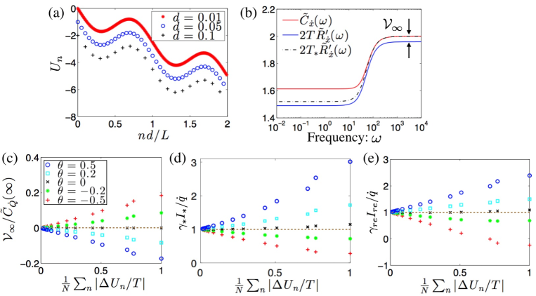
Figure S1: (a) The energy landscape $U_{n}$ for the 1-d hopping model, constructed from $U(x)=-\sin(2\pi x/L)-\Delta\mu x/L$ at a given lattice constant $d$. The landscapes for different $d$’s are shifted vertically for illustration. (b) The correlation and response spectrum for the velocity $\dot{x}_{t}\equiv\dot{n}_{t}d$, obtained at $d=0.1$ and $\theta=-0.2$. The FDT is restored in the high frequency limit with the renormalized temperature. (c) The relative high-frequency-limit violation of FDT against the average entropic change in the environment per jump: $\frac{1}{N}\sum_{n}|\Delta U_{n}/T|$. (d)(e) Emergence of the renormalized HS equality at small medium entropy production per jump. Other parameters: $w_{0}=1/d^{2}$, $T=1$, $L=1$, $\Delta\mu=2.5$, and $h=0$.

Finally, we focus on the multi-dimensional hopping models in Fig. 1(b)(c) in the main text, where the same value of $\mathcal{Q}_{p}=pd$ is shared by all the states within the same colored block. The perturbed rates of the red transitions that change the observable are assumed to satisfy

$$\tilde{w}_{m}^{n} = w_{0}\exp\Big{(}(\theta+\frac{1}{2})\Big{[}\epsilon_{m}^{n}+h\frac{\mathcal{Q}_{n}-\mathcal{Q}_{m}}{T}\Big{]}\Big{)},$$ (S17a)

$$\tilde{w}_{n}^{m} = w_{0}\exp\Big{(}(\theta-\frac{1}{2})\Big{[}\epsilon_{m}^{n}+h\frac{\mathcal{Q}_{n}-\mathcal{Q}_{m}}{T}\Big{]}\Big{)},$$ (S17b)

which essentially mimics Eq. (10), except that we do not assume an energy landscape $U_{n}$. The dissipation rate through the stochastic trajectory $Q_{t}$ is defined to be

$$\dot{q}\equiv T\sum_{n,m}(1-\delta_{\mathcal{Q}_{n}\mathcal{Q}_{m}})J_{n}^{m}\epsilon_{n}^{m},$$ (S18)

where $\epsilon_{n}^{m}=\ln[\omega_{n}^{m}/\omega_{m}^{n}]$ is the environment’s entropy production for the transition from state $n$ to $m$, and $(1-\delta_{\mathcal{Q}_{n}\mathcal{Q}_{m}})$ is a weight that only counts transitions that change the observable. Assuming that both $\epsilon_{n}^{m}$ and its relative variation are small along the direction of red transitions, the renormalized HS equality also emerges. The differences of network topologies are captured by the effective friction coefficient $\gamma_{*}=4T/(kw_{0}d^{2})$, with $k$ being the number of red transitions out of a node.

References

(1)
S. Toyabe and M. Sano,
J. Phys. Soc. Jpn. 84, 102001 (2015).
(2)
I. A. Martínez, É. Roldán, L. Dinis, and R. A. Rica, Soft
matter 13, 22 (2017).
(3)
S. Ciliberto, Phys. Rev. X 7, 021051 (2017).
(4)
R. Kubo, Rep. Prog. Phys. 29, 255 (1966).
(5)
L. F. Cugliandolo, D. S. Dean, and J. Kurchan, Phys. Rev. Lett. 79, 2168 (1997).
(6)
L. F. Cugliandolo, J. Kurchan, and L. Peliti, Phys. Rev. E 55, 3898 (1997).
(7)
P. Martin, A. Hudspeth, and F. Jülicher, Proc. Natl.
Acad. Sci. U.S.A. 98, 14380 (2001).
(8)
D. Mizuno, C. Tardin, C. Schmidt, and F. MacKintosh,
Science 315, 370 (2007).
(9)
M. Baiesi, C. Maes, and B. Wynants, Phys. Rev. Lett.
103, 010602 (2009).
(10)
U. Seifert and T. Speck, Europhys. Lett. 89, 10007
(2010).
(11)
M. Baiesi and C. Maes, New J. Phys. 15, 013004 (2013).
(12)
T. Speck and U. Seifert, Europhys. Lett. 74, 391 (2006).
(13)
J. Prost, J.-F. Joanny, and J.M.R. Parrondo, Phys. Rev. Lett.
103, 090601 (2009).
(14)
T. Harada and S.-i. Sasa, Phys. Rev. Lett. 95, 130602
(2005).
(15)
T. Harada and S.-i. Sasa, Phys. Rev. E 73, 026131 (2006).
(16)
T. Harada and S.-i. Sasa, Math. Biosci. 207, 365 (2007).
(17)
S. Toyabe and E. Muneyuki, New J. Phys. 17,
015008 (2015).
(18)
S. Toyabe, T. Okamoto, T. Watanabe-Nakayama,
H. Taketani, S. Kudo, and E. Muneyuki, Phys. Rev.
Lett. 104, 198103 (2010).
(19)
S.-W. Wang, K. Kawaguchi, S.-i. Sasa, and L.-H. Tang,
Phys. Rev. Lett. 117, 070601 (2016).
(20)
S.-W. Wang, K. Kawaguchi, S.-i. Sasa, and L.-H. Tang,
arXiv:1610.00120 (2016).
(21)
J. M. Deutsch and O. Narayan, Phys. Rev. E 74, 026112
(2006).
(22)
É. Fodor, C. Nardini, M. E. Cates, J. Tailleur, P. Visco,
and F. van Wijland, Phys. Rev. Lett. 117, 038103
(2016).
(23)
C. Nardini, É. Fodor, E. Tjhung, F. van Wijland,
J. Tailleur, and M. E Cates,
Phys. Rev. X 7, 021007 (2017).
(24)
E. Lippiello, M. Baiesi, and A. Sarracino, Phys. Rev.
Lett. 112, 140602 (2014).
(25)
E. Zimmermann and U. Seifert, New J. Phys.
14, 103023 (2012).
(26)
K. Kawaguchi, S.-i. Sasa, and T. Sagawa, Biophys. J.
106, 2450 (2014).
(27)
E. Zimmermann and U. Seifert, Phys. Rev. E 91, 022709
(2015).
(28)
A. I. Brown and D. A. Sivak, Proc. Natl.
Acad. Sci. U.S.A., 201707534 (2017).
(29)
Y. Taniguchi, M. Nishiyama, Y. Ishii, and T. Yanagida,
Nat. Chem. Biol. 1, 342 (2005).
(30)
T. Ariga, M. Tomishige, and D. Mizuno, arXiv preprint
arXiv:1704.05302 (2017).
(31)
G. Diezemann, Phys. Rev. E 72, 011104 (2005).
(32)
C. Maes and B. Wynants, Markov Process. Relat. 16, 45 (2010).
(33)
N. G. Van Kampen, Stochastic processes in physics and
chemistry, Vol. 1 (Elsevier, 1992).
(34)
See Supplemental Material for deriving the correlation and response spectrum Eq. (5), the violation formula (9), and more details about deriving the renormalized Harada-Sasa equality (14).
(35)
We note that in this system due to its finite state space. However, we expect Eq. (9) to work even for systems with an infinite state space, as suggested by our analytical and numerical examples.
(36)
S.-W. Wang, Y. Lan, and L.-H. Tang, J. Stat. Mech.
2015, P07025 (2015).