Fast Fréchet Distance Between Curves with Long Edges

Abstract.

Computing the Fréchet distance between two polygonal curves takes roughly quadratic time. In this paper, we show that for a special class of curves the Fréchet distance computations become easier. Let $P$ and $Q$ be two polygonal curves in ${\mathbb{R}}^{d}$ with $n$ and $m$ vertices, respectively. We prove four results for the case when all edges of both curves are long compared to the Fréchet distance between them: (1) a linear-time algorithm for deciding the Fréchet distance between two curves, (2) an algorithm that computes the Fréchet distance in $O((n+m)\log(n+m))$ time, (3) a linear-time $\sqrt{d}$-approximation algorithm, and (4) a data structure that supports $O(m\log^{2}n)$-time decision queries, where $m$ is the number of vertices of the query curve and $n$ the number of vertices of the preprocessed curve.

1. Introduction

Measuring the similarity between two curves is an important problem that has applications in many areas, e.g., in morphing [12], movement analysis [13], handwriting recognition [21] and protein structure alignment [19]. Fréchet distance is one of the most popular similarity measures which has received considerable attentions in recent years. It is intuitively the minimum length of the leash that connects a man and dog walking across the curves without going backward. The classical algorithm for computing the Fréchet distance between curves with total complexity $n$ runs in $O(n^{2}\log n)$ time [2]. The major goal of this paper is to focus on computing the Fréchet distance for a reasonable special class of curves in significantly faster than quadratic time.

1.1. Related Work

Buchin et al. [7] gave an $\Omega(n\log n)$ lower bound for computing the Fréchet distance. Then Bringmann [5] showed that, assuming the Strong Exponential Time Hypothesis, the Fréchet distance cannot be computed in strongly subquadratic time, i.e., in time $O(n^{2-\epsilon})$ for any $\epsilon>0$. For the discrete Fréchet distance, which considers only distances between the vertices, Agarwal et al. [1] gave an algorithm with a (mildly) subquadratic running time of $O(n^{2}\frac{\log\log n}{\log n})$. Buchin et al. [8] showed that the continuous Fréchet distance can be computed in $O(n^{2}\sqrt{\log n}(\log\log n)^{3/2})$ expected time. Bringmann and Mulzer [6] gave an $O(n^{2}/\phi+n\log n)$-time algorithm to compute a $\phi$-approximation of the discrete Fréchet distance for any integer $1\leq\phi\leq n$. Therefore, an $n^{\epsilon}$-approximation, for any $\epsilon>0$, can be computed in (strongly) subquadratic time. For the continuous Fréchet distance, there are also a few subquadratic algorithms known for restricted classes of curves such as $\kappa$-bounded, backbone and $c$-packed curves. Alt et al. [3] considered $\kappa$-bounded curves and they gave an $O(n\log n)$ time algorithm to $(\kappa+1)$-approximate the Fréchet distance. A curve $P$ is $\kappa$-bounded if for any two points $x,y\in P$, the union of the balls with radii $r$ centered at $x$ and $y$ contains the whole $P[x,y]$ where $r$ is equal to $(\kappa/2)$ times the Euclidean distance between $x$ and $y$. For any $\epsilon>0$, Aronov et al. [4] provided a near-linear time $(1+\epsilon)$-approximation algorithm for the discrete Fréchet distance for so-called backbone curves that have essentially constant edge length and require a minimum distance between non-consecutive vertices. For $c$-packed curves a $(1+\epsilon)$-approximation can be computed in $O(cn/\epsilon+cn\log n)$ time [11]. A curve is $c$-packed if for any ball $B$, the length of the portion of $P$ contained in $B$ is at most $c$ times the diameter of $B$.

1.2. Our Contribution

In this paper, we study a new class of curves, namely curves with long edges, and we show that for these curves the Fréchet distance can be computed significantly faster than quadratic time. In a particular application, one might be interested in detecting groups of different movement patterns in migratory birds that fly very long distances. As shown in Fig. 1, different flyways are comparatively straight and the trajectory data of individual birds usually consists of only one GPS sample per day in order to conserve battery power. Infrequent sampling and the straight flyways therefore result in curves with long edges, and it is desirable to compare the routes of different animals in order to identify common flyways.

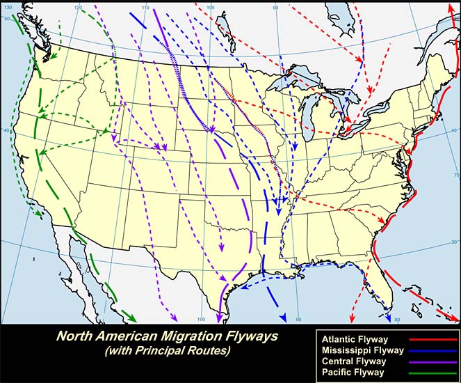
Figure 1. There are four typical flyways across the US. Clustering the trajectories by similarity between them allows us to detect the most common movement pattern [20].

We consider the decision, optimization, approximation and data structure problems for the Fréchet distance between two polygonal curves $P$ and $Q$ in ${\mathbb{R}}^{d}$ with $n$ and $m$ vertices, respectively, all for the case where all edges of both curves are long compared to the Fréchet distance between them. In Section 3 we present a greedy linear-time algorithm for deciding whether the Fréchet distance is at most $\varepsilon$, as long as all edges in $P$ are longer than $2\varepsilon$ and edges in $Q$ are longer than $(1+\sqrt{d})\varepsilon$. In Section 4 we give an algorithm for computing the Fréchet distance in $O((n+m)\log(n+m))$ time and a linear-time algorithm for approximating the Fréchet distance up to a factor of $\sqrt{d}$. In Section 5 we present a data structure that decides whether the Fréchet distance  between a preprocessed curve $P$ and a query curve $Q$ is at most $\varepsilon$ or not, in $O(m\log^{2}n)$ query time using $O(n\log n)$ space and preprocessing time.

2. Preliminaries

In this section we provide notations and definitions that will be required in the next sections. Let $P:[1,n]\rightarrow{\mathbb{R}}^{d}$ and $Q:[1,m]\rightarrow{\mathbb{R}}^{d}$ be two polygonal curves with vertices $p_{1},\ldots,p_{n}$ and $q_{1},\ldots,q_{m}$, respectively. We treat a polygonal curve as a continuous map $P:[1,n]\rightarrow\mathbb{R}^{d}$ where $P(i)=p_{i}$ for an integer $i$, and the $i$-th edge is linearly parametrized as $P(i+\lambda)=(1-\lambda)p_{i}+\lambda p_{i+1}$, for integer $i$ and $0<\lambda<1$. A re-parametrization $\sigma:[0,1]\rightarrow[1,n]$ of $P$ is any continuous, non-decreasing function such that $\sigma(0)=1$ and $\sigma(1)=n$. We denote a re-parametrization of $Q$ by $\theta:[0,1]\rightarrow[1,m]$. We denote the length of the shortest edge in $P$ and the length of the shortest edge in $Q$ by $l_{P}$ and $l_{Q}$, respectively. For two points $x,y\in{\mathbb{R}}^{d}$, let $\|x-y\|$ denote the Euclidean distance between the points and $\overline{xy}$ the straight line segment connecting $x$ to $y$. The Euclidean distance between $x\in{\mathbb{R}}^{d}$ and an edge $e:[1,2]\rightarrow{\mathbb{R}}^{d}$ is denoted as $\|x,e\|=\min_{1\leq t\leq 2}\|x-e(t)\|$. For $1\leq a\leq b\leq n$, $P[a,b]$ denotes the subcurve of $P$ starting in $P(a)$ and ending in $P(b)$. Let $\varepsilon>0$ be a real number. Consider an edge $e:[1,2]\rightarrow{\mathbb{R}}^{d}$ of length $\|e\|>2\varepsilon$ whose endpoints are $e_{1}$ and $e_{2}$. The direction vector of $e$ is the vector from $e_{1}$ to $e_{2}$. Now let $B(p,\varepsilon)=\{x\in{\mathbb{R}}^{d}\;|\;\|p-x\|\leq\varepsilon\}$ be the ball with radius $\varepsilon$ that is centered at a point $p$. The cylinder $C(e,\varepsilon)$ is the set of points in ${\mathbb{R}}^{d}$ within distance $\varepsilon$ from $e$, i.e., $C(e,\varepsilon)=\cup_{x\in e}B(x,\varepsilon)$. We say $P$ is $(e,\varepsilon)$-monotone if (1) $p_{1}\in B(e_{1},\varepsilon)$ and $p_{n}\in B(e_{2},\varepsilon)$, (2) $P\subseteq C(e,\varepsilon)$, and (3) $P$ is monotone with respect to the line supporting $e$. A curve is monotone with respect to a line $l$ if it intersects any hyperplane perpendicular to $l$ in at most one component.

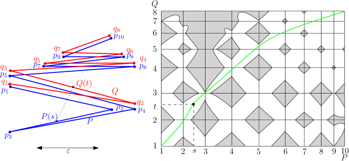
Figure 2. Two curves $P,Q$ and $\varepsilon>0$ on the left, and the free space diagram $\mathcal{FSD}_{\leq\varepsilon}$$(P,Q)$ on the right showing free space in white and blocked space in gray. A reachable path is shown in green. The point $(s,t)$ lies in free space. There is a quadratic number of cells containing free space as well as a quadratic number of cells containing blocked space in $\mathcal{FSD}_{\leq\varepsilon}$$(P,Q)$ and all of them may need to be checked to decide reachability for $(n,m)$. Note that both $P$ and $Q$ contain short edges as well as long edges compared to $\varepsilon$.

2.1. Fréchet Distance and Free-Space Diagram

To compute the Fréchet distance between $P$ and $Q$, Alt and Godau [2] introduced the notion of free-space diagram. For any $\varepsilon>0$, we denote the free-space diagram between $P$ and $Q$ by $\mathcal{FSD}_{\leq\varepsilon}$$(P,Q)$. This diagram has the domain $[1,n]\times[1,m]$ and it consists of $(n-1)\times(m-1)$ cells, where each point $(s,t)$ in the diagram corresponds to two points $P(s)$ and $Q(t)$. A point $(s,t)$ in $\mathcal{FSD}_{\leq\varepsilon}$$(P,Q)$ is called free if $\|P(s)-Q(t)\|\leq\varepsilon$ and blocked, otherwise. The union of all free points is referred to as the free space. A monotone matching between $P$ and $Q$ is a pair of re-parameterizations $(\sigma,\theta)$ corresponding to an $xy$-monotone path from $(1,1)$ to $(n,m)$ within the free space in $\mathcal{FSD}_{\leq\varepsilon}$$(P,Q)$. The Fréchet distance between two curves is defined as $\delta_{F}(P,Q)=\inf_{(\sigma,\theta)}\max_{0\leq t\leq 1}\|P(\sigma(t))-Q(\theta(t))\|$, where $(\sigma,\theta)$ is a monotone matching and $\max_{0\leq t\leq 1}\|P(\sigma(t))-Q(\theta(t))\|$ is called the width of the matching. A monotone matching realizing $\delta_{F}(P,Q)$ is called a Fréchet matching. A point $(s,t)$ is reachable if there exists a Fréchet matching from $(1,1)$ to $(s,t)$ in $\mathcal{FSD}_{\leq\varepsilon}$$(P,Q)$. A Fréchet matching in $\mathcal{FSD}_{\leq\varepsilon}$$(P,Q)$ from $(1,1)$ to $(s,t)$ is also called a reachable path for $(s,t)$ (see Fig. 2). Alt and Godau [2] compute a reachable path by propagating reachable points across free space cell boundaries in a dynamic programming manner, which requires the exploration of the entire $\mathcal{FSD}_{\leq\varepsilon}$$(P,Q)$ and takes $O(mn)$ time.

2.2. The Main Idea

We set out to provide faster algorithms for the Fréchet distance using implicit structural properties of the free-space diagram of curves with long edges. These properties allow us to develop greedy algorithms that construct valid re-parameterizations by repeatedly computing a maximally reachable subcurve on one of the curves. Like the greedy algorithm proposed by Bringmann and Mulzer [6], we compute prefix subcurves that have a valid Fréchet distance. However, while the approximation ratio of their greedy algorithm is exponential, the approximation ratio of the algorithm we present in Section 4.2 is constant, because we can take advantage of the curves having long edges. Our assumption on edge lengths is more general than backbone curves, since we do not require that non-consecutive vertices be far away from each other and we do not require any upper bound on the length of the edges.

The free space diagram for curves with long edges is simpler, and intuitively seems to have fewer reachable paths (see Fig. 3). In the remainder of this paper we show that indeed we can exploit this simpler structure to compute reachable paths in a simple greedy manner which results in runtimes that are significantly faster than quadratic.

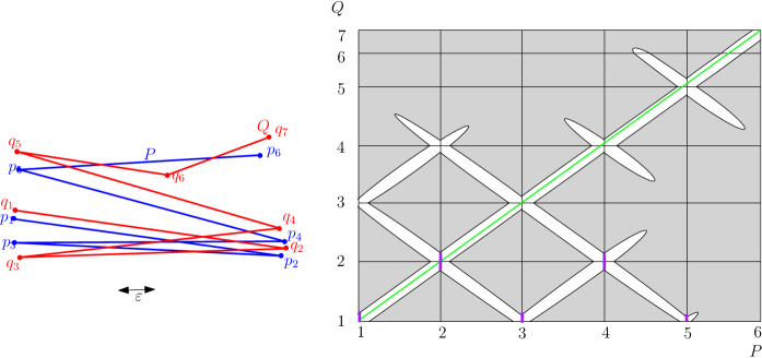
Figure 3. $\mathcal{FSD}_{\leq\varepsilon}$$(P,Q)$ for curves with long edges results in fewer reachable paths for $(n,m)$. Consider the vertical free intervals (shown in purple) in the first row of the free space diagram. Since $l_{P}>2\varepsilon$, no consecutive purple intervals intersect which is a property we exploit. One can use such a property to find a reachable path without needing to check the entire free space diagram.

3. A Greedy Decision Algorithm

In this section we give a linear time algorithm for deciding whether the Fréchet distance between two polygonal curves $P$ and $Q$ in ${\mathbb{R}}^{d}$ with relatively long edges is at most $\varepsilon$. In Section 3.1, we first prove a structural property for the case that each edge in $P$ is longer than $2\varepsilon$ and $Q$ is a single segment. Afterwards in Section 3.2, we consider the extension to the case that $P$ and $Q$ are two polygonal curves and we show some extended structural property of free space induced by two curves with long edges. In Section 3.3, we present our greedy algorithm, which is based on computing longest reachable prefixes in $P$ with respect to each segment in $Q$. We consider three different variants of edge lengths assumption when $l_{P}>2\varepsilon$ and $l_{Q}>(1+\sqrt{d})\varepsilon$ (Section 3.3.1), $l_{P}\geq 2\varepsilon$ and $l_{Q}\geq(1+\sqrt{d})\varepsilon$ (Section 3.3.2), and $l_{P}>0$ and $l_{Q}>4\varepsilon$ (Section 3.3.3). In Section 3.4, we provide a critical example for which our greedy algorithm fails when the assumption on the edge lengths does not hold.

3.1. A Simple Fréchet Matching for a Single Segment

In this section we start by introducing the crucial notion of orthogonal matching between a polygonal curve $P$ and a single line segment $e$. An orthogonal matching projects each point from $P$ to its closest point on $e$. In particular, it maps vertices of $P$ either orthogonally to the segment $e$ or directly to the endpoints of $e$.

Definition 3.1 (Orthogonal Matching).

Let $\varepsilon>0$, $P:[1,n]\rightarrow\mathbb{R}^{d}$ be a polygonal curve, and $e:[1,2]\rightarrow\mathbb{R}^{d}$ be a line segment. A Fréchet matching $(\sigma,\theta)$ realizing $\delta_{F}(P,e)\leq\varepsilon$ is called an orthogonal matching of width at most $\varepsilon$ if $\sigma(t)=1$ for $t\in[0,a]$, $\|P(\sigma(t))-e(\theta(t))\|=\|P(\sigma(t)),e\|\leq\varepsilon$ for $t\in(a,b)$, and $\sigma(t)=n$ for $t\in[b,1]$ for some $0\leq a\leq b\leq 1$; see Fig. 4(a).

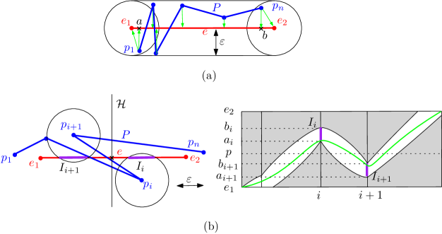
Figure 4. (a) In this example $P$ is $(e,\varepsilon)$-monotone and the green arrows indicate an orthogonal matching between $P$ and $e$. (b) An illustration of the case ${\cal H}\cap e\neq\emptyset$ in the proof of (1) $\Rightarrow$ (2) in Lemma 3.2. Note that the consecutive purple intervals $I_{i}$ and $I_{i+1}$ do not intersect because $l_{P}>2\varepsilon$.

Now we state a key lemma that demonstrates that if $P$ has long edges, then the orthogonal matching of width at most $\varepsilon$ between $P$ and a segment $e$ exists if and only if $\delta_{F}(P,e)\leq\varepsilon$, and this is equivalent to $P$ being $(e,\varepsilon)$-monotone.

Lemma 3.2 (Orthogonal Matching and Monotonicity).

Let $\varepsilon>0$, $P:[1,n]\rightarrow\mathbb{R}^{d}$ be a polygonal curve and $e:[1,2]\rightarrow\mathbb{R}^{d}$ be a line segment. Consider the following statements:

1. $\delta_{F}(P,e)\leq\varepsilon$,

2. $P$ is $(e,\varepsilon)$-monotone,

3. $P$ and $e$ admit an orthogonal matching of width at most $\varepsilon$.

In general, (2) $\Leftrightarrow$ (3) and (3) $\Rightarrow$ (1). In addition, if $l_{P}>2\varepsilon$ then (1) $\Rightarrow$ (2), i.e., all three statements are equivalent.

Proof 3.3.

We immediately have (3) $\Rightarrow$ (1) by Definition 3.1. To prove (2) $\Rightarrow$ (3), assume $P$ is $(e,\varepsilon)$-monotone. We can construct an orthogonal matching by mapping each $p_{i}$ to its nearest neighbor $e(1+t_{i})$ on $e$, with $0\leq t_{i-1}\leq t_{i}\leq 1$. We set $\sigma(t_{i})=i$ and $\theta(t_{i})=1+t_{i}$ for all $i=1,\ldots,n$, and we set $a=t_{1}$, $b=t_{n}$, $\sigma(t)=1$ for $t\in[0,a]$, $\sigma(t)=n$ for $t\in[b,1]$, and $\theta(0)=1$ and $\theta(1)=2$. The matching $(\sigma,\theta)$ is obtained by linearly interpolating between these values. The function $\sigma(t)$ is monotone by construction, and $\theta(t)$ is monotone because $P$ is monotone with respect to the line supporting $e$. And all distances $\|P(\sigma(t))-e(\theta(t))\|\leq\varepsilon$ because $P$ is $(e,\varepsilon)$-monotone. Thus $(\sigma,\theta)$ is an orthogonal matching of width at most $\varepsilon$. To prove (3) $\Rightarrow$ (2), let $(\sigma,\theta)$ be an orthogonal matching of width at most $\varepsilon$. Then clearly $p_{1}\in B(e_{1},\varepsilon)$, $p_{n}\in B(e_{2},\varepsilon)$, and $P\subseteq C(e,\varepsilon)$. Let $t_{1},\ldots,t_{n}$ be such that $P(\sigma(t_{i}))=p_{i}$ for $i=1,\ldots,n$. Since $(\sigma,\theta)$ is a (monotone) Fréchet matching, $\theta(t_{1}),\ldots,\theta(t_{n})$ is a monotone increasing sequence. And since $(\sigma,\theta)$ is orthogonal, the line segments $\overline{p_{i}\theta(t_{i})}$ are all monotone to the line $\ell$ supporting $e$. Therefore, $P$ is monotone with respect to $\ell$ and thus $P$ is $(e,\varepsilon)$-monotone.

Now assume $l_{P}>2\varepsilon$. In order to prove (1) $\Rightarrow$ (2), if $\delta_{F}(P,e)\leq\varepsilon$ then clearly $p_{1}\in B(e_{1},\varepsilon)$, $p_{n}\in B(e_{2},\varepsilon)$, and $P\subseteq C(e,\varepsilon)$. It remains to show that $P$ is monotone with respect to the line $\ell$ supporting $e$. For all $i=1,\ldots,n$, define $I_{i}=B(p_{i},\varepsilon)\cap e=e[a_{i},b_{i}]$. Because $l_{P}>2\varepsilon$, we know that $I_{i}\cap I_{i+1}=\emptyset$. Let $(\sigma,\theta)$ be a monotone matching realizing $\delta_{F}(P,e)\leq\varepsilon$. For the sake of contradiction assume there exists a hyperplane ${\cal H}$ perpendicular to $\ell$ such that $P$ intersects ${\cal H}$ in at least two points $P(x)$ and $P(y)$, where $x<y$. Let $p_{i}$ be the last vertex along $P[x,y]$, and recall that $e_{1}$ and $e_{2}$ are the two vertices of $e$. First assume that ${\cal H}\cap e\neq\emptyset$. Then $p_{i}$ lies on the $e_{2}$-side of ${\cal H}$ and $p_{i+1}$ lies on the $e_{1}$-side of ${\cal H}$. Therefore, because $I_{i}\cap I_{i+1}=\emptyset$, we know that $a_{i}>b_{i+1}$. Let $t_{i},t_{i+1}\in[0,1]$ be two values such that $p_{i}=P(\sigma(t_{i}))$ and $p_{i+1}=P(\sigma(t_{i+1}))$, where $t_{i}<t_{i+1}$. From $\sigma(t_{i})\geq a_{i}$ and $\sigma(t_{i+1})\leq b_{i+1}$, we know that $\sigma(t_{i})>\sigma(t_{i+1})$, which violates the monotonicity of $(\sigma,\theta)$, see Fig. 4(b). Now consider the case that ${\cal H}\cap e=\emptyset$. Then $p_{i}$ lies on one side of ${\cal H}$, and $e$ lies entirely on the other side. If ${\cal H}\cap B(e_{1},\varepsilon)\neq\emptyset$, then we know that $P[1,y]\subseteq B(e_{1},\varepsilon)$. But this is not possible since all edges of $P$ are longer than $2\varepsilon$. The same argument holds if ${\cal H}\cap B(e_{2},\varepsilon)\neq\emptyset$.

In fact Lemma 3.2 shows that for a curve $P$ with long edges, the Fréchet distance to a line segment $e$ is determined by examining whether $P$ is $(e,\varepsilon)$-monotone or not.

3.2. A Simple Fréchet Matching for More than One Segment

In this section, we extend the matching between a curve $P$ and a single line-segment $e$ to a matching between two curves $P$ and $Q$.

Definition 3.4 (Longest $\varepsilon$-Prefix).

Let $\varepsilon>0$, $P:[1,n]\rightarrow\mathbb{R}^{d}$ be a polygonal curve, and $e:[1,2]\rightarrow\mathbb{R}^{d}$ be a line segment. Define $\gamma=\max\{\,t\;|\;1\leq t\leq n\;\mbox{and}\;\delta_{F}(P[1,t],e)\leq\varepsilon\}$. We call $P[1,\gamma]$ the longest $\varepsilon$-prefix of $P$ with respect to $e$.

We now use the longest $\varepsilon$-prefix to define an extension of the matching introduced in Definition 3.1. Definition 3.4 is the basis of our greedy algorithm (Algorithm 1) which is presented in the next section. We show that if there exists a matching between two curves, then one can necessarily cut it into $m-1$ orthogonal matchings between each segment in $Q$ and the corresponding longest $\varepsilon$-prefix. Before we reach this property, we need the following technical lemma:

Lemma 3.5 ($(\sqrt{d}\varepsilon)$-Ball).

Let $\varepsilon>0$ and let $P:[1,n]\rightarrow\mathbb{R}^{d}$ be a polygonal curve such that $l_{P}>2\varepsilon$. Let $e:[1,2]\rightarrow\mathbb{R}^{d}$ where $\|e\|>2\varepsilon$. Assume that $P[1,\gamma]$ is the longest $\varepsilon$-prefix of $P$ with respect to $e$, and let $\alpha$ be a parameter such that $P(\alpha)$ is the first point along $P$ that intersects $B(e_{2},\varepsilon)$. Then $P[\alpha,\gamma]\subseteq B(e_{2},\sqrt{d}\varepsilon)$.

Proof 3.6.

By assumption $\|e\|>2\varepsilon$, we know that $B(e_{1},\varepsilon)\cap B(e_{2},\varepsilon)=\emptyset$, thus $\alpha$ exists. Notice that $P[\alpha,\gamma]\subseteq C(e,\varepsilon)$. Let ${\cal H}$ be the hyperplane that is intersecting and perpendicular to $e$ and is tangent to $B(e_{2},\varepsilon)$. Hence ${\cal H}$ splits $P[1,\gamma]$ into two parts, the part on the $e_{1}$-side and the part that on the $e_{2}$-side. Let $P(x)$ be the last vertex before $P(\gamma)$ along $P$. By Definition 3.4, $\delta_{F}(P[1,\gamma],e)\leq\varepsilon$, and (1) if $P(x)\in B(e_{2},\varepsilon)$, then Lemma 3.2 implies that $P[1,x]$ is $(e,\varepsilon)$-monotone. Thus $P[\alpha,\gamma]$ must lie on the $e_{2}$-side of ${\cal H}_{2}$, and in particular inside the cube enclosing $B(e_{2},\varepsilon)$, see Fig. 5. Therefore the maximum possible distance between any point in $P[\alpha,\gamma]$ and $e_{2}$ is $\sqrt{d}\varepsilon$. (2) If $P(x)\notin B(e_{2},\varepsilon)$, we first show that $P[1,x]$ is monotone with respect to the line supporting $e$ and then we use the similar argument as in (1) to imply the maximum possible distance between any point in $P[\alpha,\gamma]$ and $e_{2}$ is $\sqrt{d}\varepsilon$. Now let $(\sigma,\theta)$ be a Fréchet matching between $P[1,\gamma]$ and $e$. For the sake of contradiction assume there exists an edge $P[i,i+1]$ such that the angle between the direction vectors of $P[i,i+1]$ and $e$ is greater than $\pi/2$ with $i<x$. Let $t_{i},t_{i+1}\in[0,1]$ be two real values with $t_{i}<t_{i+1}$ such that $\sigma(t_{i})=i$ and $\sigma(t_{i+1})=i+1$ and let $I_{i}=B(p_{i},\varepsilon)\cap e=e[a_{i},b_{i}]$ and $I_{i+1}=B(p_{i+1},\varepsilon)\cap e=e[a_{i+1},b_{i+1}]$. Now from $B(p_{i},\varepsilon)\cap B(p_{i+1},\varepsilon)=\emptyset$ follows that $I_{i}\cap I_{i+1}=\emptyset$. Note that the angle between the direction vectors of $P[i,i+1]$ and $e$ is greater than $\pi/2$ which indicates that $b_{i+1}<a_{i}$. Therefore $a_{i+1}\leq\theta(t_{i+1})\leq b_{i+1}<a_{i}\leq\theta(t_{i})\leq b_{i}$. Now three following cases are expected: (i) if $i+1<\alpha$, then $\gamma$ does not exist since $(\sigma,\theta)$ is not monotone and this would be a contradiction. Therefore $P[1,x]$ is monotone with respect to the line supporting $e$. (ii) If $\alpha<i\leq x$, then $\gamma<x$ since $i<\gamma<i+1$ which is a contradiction with $\gamma>x$. Hence $P[1,x]$ is monotone with respect to the line supporting $e$. (iii) if $i=x\leq\alpha$, then $P[\alpha,\gamma]$ is only a subsegment of $P[i,i+1]$ and trivially lies within $B(e_{2},\varepsilon)$. This completes the proof.

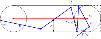
Figure 5. The farthest point in $P[\alpha,\gamma]$ from $e_{2}$ must lie inside the cube enclosing $B(e_{2},\varepsilon)$.

Lemma 3.7 (($3\varepsilon)$-Ball).

Let $\varepsilon>0$ and let $P:[1,n]\rightarrow\mathbb{R}^{d}$ be a polygonal curve. Let $e:[1,2]\rightarrow\mathbb{R}^{d}$ where $\|e\|>2\varepsilon$. Assume that $P[1,\gamma]$ is the longest $\varepsilon$-prefix of $P$ with respect to $e$ and $P(\alpha)$ is the first point along $P$ that intersects $B(e_{2},\varepsilon)$. Then $P[\alpha,\gamma]\subseteq B(e_{2},3\varepsilon)$.

Proof 3.8.

Although the proof of Lemma 11 in Gudmundsson and Smid [17] is similar, we describe a slight modification of the proof that is necessary for our setting. Suppose $(\sigma,\theta)$ is a Fréchet matching realizing $\delta_{F}(P[1,\gamma],e)\leq\varepsilon$. Let $x\in[\alpha,\gamma]$ such that $P(x)$ is the farthest point to $e_{2}$. We need to show that $\|P(x)-e_{2}\|\leq 3\varepsilon$ which implies $P[\alpha,\gamma]\subseteq B(e_{2},3\varepsilon)$. Let $t_{\alpha},t_{\gamma}\in[0,1]$ be two values such that $\alpha=\sigma(t_{\alpha})$ and $\gamma=\sigma(t_{\gamma})$. Note that there exists some $t_{x}\in[t_{\alpha},t_{\gamma}]$ such that $x=\sigma(t_{x})$. By the triangle inequality we have:

$$\|P(x)-e_{2}\|\leq\|P(x)-e(\theta(t_{x}))\|+\|e(\theta(t_{x}))-e_{2}\|\leq\varepsilon+\|e(\theta(t_{x}))-e_{2}\|.$$

Note that $t_{x}>t_{\alpha}$ and we can have $\|e(\theta(t_{x}))-e_{2}\|\leq\|e(\theta(t_{\alpha}))-e_{2}\|$, hence:

$$\|P(x)-e_{2}\|\leq\varepsilon+\|e(\theta(t_{\alpha}))-e_{2}\|.$$

By applying the triangle inequality once more we have:

$$\|P(x)-e_{2}\|\leq\varepsilon+\|e(\theta(t_{\alpha}))-P(\alpha)\|+\|P(\alpha)-e_{2}\|\leq 3\varepsilon.$$

Now we show that if $\delta_{F}(P,Q)\leq\varepsilon$, then the two polygonal curves $P$ and $Q$ admit a piecewise orthogonal matching, which can be obtained by computing longest $\varepsilon$-prefixes of $P$ with respect to each segment of $Q$. This lemma is the foundation of our greedy algorithm (Algorithm 1).

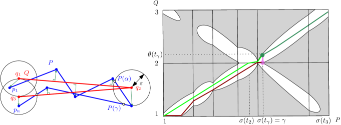
Figure 6. Given an arbitrary matching (the concatenation of the light and dark green reachable paths), the orthogonal matching (the brown reachable path) between $P[1,\gamma]$ and $Q[1,2]$ exists. We construct a matching realizing $\delta_{F}(P[\gamma,n],Q[2,m])\leq\varepsilon$ as the concatenation of the pink and the dark green reachable paths.

Lemma 3.9 (Cutting Lemma).

Let $\varepsilon>0$, and let $P:[1,n]\rightarrow\mathbb{R}^{d}$ and $Q:[1,m]\rightarrow\mathbb{R}^{d}$ be two polygonal curves such that $l_{P}>2\varepsilon$ and $l_{Q}>(1+\sqrt{d})\varepsilon$. If $\delta_{F}(P,Q)\leq\varepsilon$, then $P[1,\gamma]$ as the longest $\varepsilon$-prefix of $P$ with respect to $Q[1,2]$ exists, $\delta_{F}(P[1,\gamma],Q[1,2])\leq\varepsilon$ and $\delta_{F}(P[\gamma,n],Q[2,m])\leq\varepsilon$.

Proof 3.10.

Let $(\sigma,\theta)$ be any Fréchet matching realizing $\delta_{F}(P,Q)\leq\varepsilon$. This corresponds to a reachable path, which is shown as the concatenation of the light and dark green paths in the example in Fig. 6. Let $t_{2}\in[0,1]$ be the largest value such that $Q({\theta(t_{2})})=q_{2}$, hence $\delta_{F}(P[1,\sigma(t_{2})],Q[1,2])\leq\varepsilon$. By Definition 3.4, $\gamma$ exists with $\gamma\geq\sigma(t_{2})$, and $\delta_{F}(P[1,\gamma],Q[1,2])\leq\varepsilon$. See the brown reachable path corresponding to the orthogonal matching realizing $\delta_{F}(P[1,\gamma],Q[1,2])\leq\varepsilon$ in Fig. 6. In the remainder of this proof we construct a matching to prove that $\delta_{F}(P[\gamma,n],Q[2,m])\leq\varepsilon$ (the concatenation of the pink and dark green paths).

Let $t_{\gamma}\in[0,1]$ be the largest value such that $P(\sigma(t_{\gamma}))=P(\gamma)$. By Lemma 3.5, $P[\sigma(t_{2}),\gamma]\subseteq B(q_{2},\sqrt{d}\varepsilon)$. Now let $t_{3}\in[0,1]$ be the smallest value such that $Q(\theta(t_{3}))=q_{3}$. We have $\|q_{2}-q_{3}\|>(1+\sqrt{d})\varepsilon$, therefore $B(q_{2},\sqrt{d}\varepsilon)\cap B(q_{3},\varepsilon)=\emptyset$ and thus $(\sigma,\theta)$ cannot match $q_{3}$ to any point in $P[\sigma(t_{2}),\gamma]$. Therefore, $\sigma(t_{2})\leq\gamma=\sigma(t_{\gamma})<\sigma(t_{3})$, and correspondingly $\theta(t_{2})\leq\theta(t_{\gamma})<\theta(t_{3})$.

Now we construct a new matching $(\bar{\sigma},\bar{\theta})$ realizing $\delta_{F}(P[\gamma,n],Q[2,m])\leq\varepsilon$ as follows: $\bar{\sigma}(t)=\sigma(t)$ and $\bar{\theta}(t)=\theta(t)$ for all $t_{\gamma}\leq t\leq 1$ (dark green reachable path). On the other hand, since $\|P(\gamma)-q_{2}\|\leq\varepsilon$ (pink point) and $\|P(\gamma)-Q({\theta(t_{\gamma})})\|\leq\varepsilon$ (dark green point), we know that $Q[2,\theta(t_{\gamma})]\subseteq B(P(\gamma),\varepsilon)$, i.e., the pink vertical segment is free. We set, $\bar{\sigma}(t)=\gamma$ and $\bar{\theta}(t)=\frac{t_{\gamma}-t}{t_{\gamma}}\cdot 2+\frac{t}{t_{\gamma}}\cdot\theta(t_{\gamma})$ for all $t_{2}\leq t\leq t_{\gamma}$ (pink reachable path). Therefore, we have $\delta_{F}(P[\gamma,n],Q[2,m])\leq\varepsilon$, which completes the proof.

Now since by Lemma 3.9 we have $\delta_{F}(P[1,\gamma],Q[1,2])\leq\varepsilon$,  Lemma 3.2 implies that the matching between $P[1,\gamma]$ and $Q[1,2]$ is orthogonal. Let $P(x)$ be the last vertex of $P[1,\gamma]$ and let $Q(x^{\prime})$ be its closest point on $Q[1,2]$, for some $x<\gamma$ and $x^{\prime}\leq 2$. Note that if $\|P(\gamma)-P(x)\|$ is shorter than $2\varepsilon$, we can adjust the orthogonal matching by simply mapping all points on $P[x,\gamma]$ to $Q[x^{\prime},2]$. In addition, if $P$ and $Q$ have long edges then the free-space diagram is simpler than in the general case, since the entire vertical space (the pink segment in Fig. 6) between the two points $(\gamma,2)$ and $(\gamma,\theta(t_{\gamma}))$ has to be free and cannot contain any blocked points.

3.3. The Decision Algorithm

In this section we present a linear time decision algorithm using the properties provided in Section 3.1 and Section 3.2. In Section 3.3.1 we consider the case that $l_{P}>2\varepsilon$ and $l_{Q}>(1+\sqrt{d})\varepsilon$. In Section 3.3.2 we show that this approach can be generalized to the case that $l_{P}\geq 2\varepsilon$ and $l_{Q}\geq(1+\sqrt{d})\varepsilon$, and in Section 3.3.3 we generalize the approach to the case that there is only an edge length assumption on $Q$.

3.3.1. Long Edges with $l_{P}>2\varepsilon$ and $l_{Q}>(1+\sqrt{d})\varepsilon$

At the heart of our decision algorithm is the greedy algorithm presented in Algorithm 1. The input to this DecisionAlgorithm are two polygonal curves $P$ and $Q$, and $\varepsilon>0$. The algorithm assumes that $P$ and $Q$ have long edges. In each iteration the function LongestEpsilonPrefix returns $\gamma$, where $P[s,\gamma]$ is the longest $\varepsilon$-prefix of $P[s,n]$ with respect to $Q[i-1,i]$, if it exists. Here, $s$ is the parameter where $P(s)$ is the endpoint of the previous longest $\varepsilon$-prefix with respect to $Q[i-2,i-1]$. At any time in the algorithm, if $\gamma=null$, this means that the corresponding longest $\varepsilon$-prefix does not exist and then “No” is returned. Otherwise, the next edge of $Q$ is processed. This continues iteratively until all edges have been processed, or $\gamma_{i}$ does not exist for some $i=2,\cdots,m$.

1

2DecisionAlgorithm($P[1,n],Q[1,m],\varepsilon$)

      

       // Assumes $l_{P}>2\varepsilon\leavevmode\nobreak\ \mbox{and}\leavevmode\nobreak\ l_{Q}>(1+\sqrt{d})\varepsilon$

3       $\gamma_{1}\leftarrow 1$

4       for $i\leftarrow 2$ to $m$ do

5             $\gamma_{i}\leftarrow$LongestEpsilonPrefix($P[\gamma_{i-1},n],Q[i-1,i],\varepsilon$)

6             if $\gamma=null$ then  return “No”

7             $s\leftarrow\gamma$

8            

9      if $\gamma<n$ then return “No”

10       return “Yes”

Algorithm 1 Decide whether $\delta_{F}(P,Q)\leq\varepsilon$

The $\textsc{LongestEpsilonPrefix}(P[\gamma_{i-1},n],Q[i-1,i],\varepsilon)$ procedure is implemented as follows: We use Alt and Godau’s [2] dynamic programming algorithm to compute the reachability information in $\mathcal{FSD}_{\leq\varepsilon}$$(P[\gamma_{i-1},n],Q[i-1,i])$, which computes all $(s,t)$ for which $\delta_{F}(P[\gamma_{i-1},s],Q[i-1,t])\leq\varepsilon$. This takes linear time in the complexity of $P[\gamma_{i-1},n]$ since $Q[i-1,i]$ is a single segment. Then $\gamma_{i}$ is the largest $s$ for which $\delta_{F}(P[\gamma_{i-1},s],Q[i-1,i])\leq\varepsilon$. Note that $P(s)$ has to lie on the boundary of $B(q_{i},\varepsilon)$. If no such $s$ exists then $\gamma_{i}=null$. We now prove the correctness of our decision algorithm.

Theorem 3.11 (Correctness).

Let $\varepsilon>0$, and let $P:[1,n]\rightarrow\mathbb{R}^{d}$ and $Q:[1,m]\rightarrow\mathbb{R}^{d}$ be two polygonal curves such that $l_{P}>2\varepsilon$ and $l_{Q}>(1+\sqrt{d})\varepsilon$. Then DecisionAlgorithm($P,Q,\varepsilon$) returns “Yes” if and only if $\delta_{F}(P,Q)\leq\varepsilon.$

Proof 3.12.

If the algorithm returns “Yes” then the sequence $\{(q_{i},\gamma_{i})\}$ for all $i=1,\ldots,m$ with $\gamma_{1}=1$ and $\gamma_{m}=n$ describes a monotone matching that realizes $\delta_{F}(P,Q)\leq\varepsilon$.

If $\delta_{F}(P,Q)\leq\varepsilon$, then we prove by induction on $i$ that the algorithm returns “Yes”, i.e., all longest $\varepsilon$-prefixes $(P[1,\gamma_{2}],P[\gamma_{2},\gamma_{3}],\ldots,P[\gamma_{m-1},\gamma_{m}])$ of $P$ with respect to the corresponding segments of $Q$ exist. For $i=2$, following Lemma 3.9, $\gamma_{2}$ exists and can be found by the algorithm. For any $i>2$, the algorithm has determined $\gamma_{2},\ldots,\gamma_{i-1}$ already and by Lemma 3.9, $\delta_{F}(P[\gamma_{i-1},n],Q[i-1,m])\leq\varepsilon$. Another application of Lemma 3.9 yields that $\delta_{F}(P[\gamma_{i-1},\gamma_{i}],Q[i-1,i])\leq\varepsilon$ and $\delta_{F}(P[\gamma_{i},n],Q[i,m])\leq\varepsilon$.

In the case that $i=m-1$ it remains to prove that $\gamma_{i+1}=\gamma_{m}=n$. For the sake of contradiction, assume $\gamma_{m}<n$. Since $P[\gamma_{m-1},\gamma_{m}]$ is the longest $\varepsilon$-prefix, there is no other $\gamma^{\prime}_{m}\in(\gamma_{m},n]$ such that $\delta_{F}(P[\gamma_{m-1},\gamma^{\prime}_{m}],Q[m-1,m])\leq\varepsilon$. Consequently, $\delta_{F}(P[\gamma_{m-1},\gamma^{\prime}_{m}],Q[m-1,m])>\varepsilon$ and therefore $\delta_{F}(P[\gamma_{m-1},n],Q[m-1,m])>\varepsilon$. Applying the contrapositive of Lemma 3.9 to $P[\gamma_{m-1},n]$ and $Q[m-1,m]$ yields $\delta_{F}(P,Q)>\varepsilon$, which is a contradiction. Therefore $\gamma_{m}=n$ and the algorithm returns “Yes” as claimed.

Observation 3.13 (Piecewise Orthogonal Matching).

If $\delta_{F}(P,Q)\leq\varepsilon$, then the sequence $\{\gamma_{1},\gamma_{2},\ldots,\gamma_{n}\}$ computed by Algorithm 1 induces a Fréchet matching that maps $P(\gamma_{i})$ to $q_{i}$, and therefore $\delta_{F}(P,Q)\leq\varepsilon$ for all $i=2,\ldots,m$.  Lemma 3.2 implies that the matching between $P[\gamma_{i-1},\gamma_{i}]$ and $Q[i-1,i]$ is orthogonal.

We summarize this section with the following theorem:

Theorem 3.14 (Runtime).

Let $\varepsilon>0$, and let $P:[1,n]\rightarrow\mathbb{R}^{d}$ and $Q:[1,m]\rightarrow\mathbb{R}^{d}$ be two polygonal curves such that $l_{P}>2\varepsilon$ and $l_{Q}>(1+\sqrt{d})\varepsilon$. Then there exists a greedy decision algorithm, Algorithm 1, that can determine whether $\delta_{F}(P,Q)\leq\varepsilon$ in $O(n+m)$ time.

Proof 3.15.

The number of vertices in $P[\gamma_{i-1},\gamma_{i}]$ is at most $\lceil\gamma_{i}-\gamma_{i-1}\rceil+1$. The algorithm greedily finds the longest $\varepsilon$-prefix per edge $Q[i-1,i]$ by calling LongestEpsilonPrefix$(P[s,n],Q[i-1,i],\varepsilon)$ in $O(\lceil\gamma_{i}-\gamma_{i-1}\rceil+1)$ time. The for-loop iterates over $m-1$ edges, thus the runtime is $\sum_{i=2}^{m}(\lceil\gamma_{i}-\gamma_{i-1}\rceil+1)<\sum_{i=2}^{m}(\gamma_{i}-\gamma_{i-1}+2)=\gamma_{m}-\gamma_{1}+2(m-1)=n-1+2m-2=O(n+m)$.

3.3.2. Long Edges with $l_{P}\geq 2\varepsilon$ and $l_{Q}\geq(1+\sqrt{d})\varepsilon$

We now consider the slightly more general case that $l_{P}\geq 2\varepsilon$ and $l_{Q}\geq(1+\sqrt{d})\varepsilon$. The optimization algorithm presented in Section 4.1 makes use of this case. Clearly, if $l_{P}>2\varepsilon$ and $l_{Q}>(1+\sqrt{d})\varepsilon$ then Theorem 3.11 applies as usual. If $l_{P}=2\varepsilon$ or $l_{Q}=(1+\sqrt{d})\varepsilon$ then Algorithm 1 can still be run, however the Fréchet matching induced by the $\gamma_{i}$ is not necessarily a piecewise orthogonal matching anymore, which means Observation 3.13 may not hold, see Fig. 7. However, we can still prove a slightly modified correctness theorem.

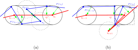
Figure 7. Two examples of matchings between $P[\gamma_{i-1},\gamma_{i}]$ and $Q[i-1,i]$ that are not (piecewise) orthogonal. Matchings are indicated with green arrows. All balls have radius $\varepsilon$. (a) An example where $l_{P}=\|p_{j+1}-p_{j}\|=2\varepsilon$ and $\gamma_{i}$ exists, but the induced Fréchet matching is not orthogonal. (b) An example where $\|q_{i+1}-q_{i}\|=(1+\sqrt{d})\varepsilon$ and $B(q_{i+1},\varepsilon)\cap B(q_{i},\sqrt{d}\varepsilon)\cap P=p_{j}$. Although $\gamma_{i}$ exists, a matching that is not piecewise orthogonal of width exactly $\varepsilon$ exists.

Theorem 3.16.

Let $\varepsilon>0$, and $l_{P}\geq 2\varepsilon$ and $l_{Q}\geq(1+\sqrt{d})\varepsilon$. If DecisionAlgorithm$(P,Q,\varepsilon)$ returns “Yes” then $\delta_{F}(P,Q)\leq\varepsilon$. If it returns “No” then $\delta_{F}(P,Q)\geq\varepsilon$.

Proof 3.17.

Let $\varepsilon^{*}=\delta_{F}(P,Q)$. If $l_{P}>2\varepsilon$ and $l_{Q}>(1+\sqrt{d})\varepsilon$ then Theorem 3.11 applies as usual. So, assume $l_{P}=2\varepsilon$ or $l_{Q}=(1+\sqrt{d})\varepsilon$. If the algorithm returns “Yes”, then we know that $\delta_{F}(P[\gamma_{i-1},\gamma_{i}],Q[i-1,i])\leq\varepsilon_{0}$ for all $i=2,\ldots,m$, and therefore $\varepsilon^{*}\leq\varepsilon$.

In the remainder of this proof we show the contrapositive of the second part: If $\varepsilon^{*}=\delta_{F}(P,Q)<\varepsilon$ then DecisionAlgorithm$(P,Q,\varepsilon)$ returns “Yes”. So, assume $\varepsilon^{*}<\varepsilon$. Then, by Theorem 3.11, DecisionAlgorithm$(P,Q,\varepsilon^{*})$ returns “Yes”, which means that all $\gamma^{*}_{i}=\textsc{LongestEpsilonPrefix}(P[\gamma^{*}_{i-1},n],Q[i-1,i],\varepsilon^{*})$ exist for all $i=2,\ldots,m$, and $\gamma^{*}_{1}=1$. We prove by induction that all $\gamma_{i}=\textsc{LongestEpsilonPrefix}(P[\gamma_{i-1},n],Q[i-1,i],\varepsilon)$ exist as well. The inductive base is trivial to show since $\gamma_{1}=\gamma^{*}_{1}=1$. Now as an inductive hypothesis let $i>1$ be the largest integer value for which $\gamma_{i-1}$ exists and is computed. In the following we show that $\gamma_{i}=\textsc{LongestEpsilonPrefix}(P[\gamma_{i-1},n],Q[i-1,i],\varepsilon)$ exists and can be computed. Let $P(x)$ be the first point along $P[\gamma^{*}_{i},n]$ on the boundary of $B(q_{i},\varepsilon)$. We have $\gamma^{*}_{i-1}<\gamma_{i-1}<\gamma^{*}_{i}<x$, where the first inequality follows from $B(q_{i-1},\varepsilon^{*})\subset B(q_{i-1},\varepsilon)$, and the second inequality follows from $B(q_{i-1},\varepsilon)\cap B(q_{i},\varepsilon^{*})=\emptyset$ because $l_{Q}>2\varepsilon$. Now let $(\sigma,\theta)$ be the Fréchet matching realizing $\delta_{F}(P[\gamma^{*}_{i-1},\gamma^{*}_{i}],Q[i-1,i])\leq\varepsilon^{*}$, and let $t\in[0,1]$ such that $\sigma(t)=\gamma_{i-1}$. Then from $\gamma^{*}_{i-1}<\gamma_{i-1}<\gamma^{*}_{i}$ follows that $i-1\leq\theta(t)\leq i$. We can therefore construct a piecewise re-parameterization for $P[\gamma_{i-1},x]$ and $Q[i-1,i]$ which yields:

$$\delta_{F}(P[\gamma_{i-1},x],Q[i-1,i]) \leq\max\{\;\delta_{F}\big{(}P(\gamma_{i-1}),Q[i-1,\theta(t)]\big{)},$$

$$\hskip 39.83385pt\delta_{F}\big{(}P[\gamma_{i-1},\gamma^{*}_{i}],Q[\theta(t),i]\big{)},\,\delta_{F}\big{(}P[\gamma^{*}_{i},x],q_{i}\big{)}\;\}\leq\varepsilon.$$

Since $\gamma_{i}\geq x$, this implies that all $\gamma_{i}$ exist for all $i=2,\ldots,m$. Note that the procedure $\textsc{LongestEpsilonPrefix}(P[\gamma_{i-1},n],Q[i-1,i])$ can compute $\gamma_{i}$ by finding the reachable path for $(\gamma_{i},i)$ across $\mathcal{FSD}_{\leq\varepsilon}$$(P[\gamma_{i-1},n],Q[i-1,i])$. Therefore DecisionAlgorithm$(P,Q,\varepsilon)$ returns “Yes”.

3.3.3. Long Edges with $l_{Q}>4\varepsilon$

Our algorithm also can be applied to the case that one curve has arbitrary edge lengths and the other curve has edge lengths greater than $4\varepsilon$.

Theorem 3.18 (Single Curve with Long Edges).

Let $\varepsilon>0$, and let $P:[1,n]\rightarrow\mathbb{R}^{d}$ and $Q:[1,m]\rightarrow\mathbb{R}^{d}$ be two polygonal curves such that $l_{P}>0$ and $l_{Q}>4\varepsilon$. Then there exists a greedy decision algorithm, Algorithm 1, that can determine whether $\delta_{F}(P,Q)\leq\varepsilon$ or $\delta_{F}(P,Q)>\varepsilon$ in $O(n+m)$ time.

Proof 3.19.

In the proof of Lemma 3.9, we can replace Lemma 3.5 with Lemma 3.7, and realize that Lemma 3.9 also holds for the case $l_{P}>0$ and $l_{Q}>4\varepsilon$. The rest follows from Theorem 3.11 and Theorem 3.14.

3.4. Necessity of the Assumption

As we have seen so far, Algorithm 1 greedily constructs a feasible Fréchet matching by linearly walking on curve $P$ to find all longest $\varepsilon$-prefixes on it with respect to the corresponding edges of $Q$. Unfortunately, this property is not always true for curves with short edges. In general, there can be a quadratic number of blocked regions in the free space diagram of two curves; see Fig. 8 as an example of two curves in ${\mathbb{R}}^{2}$ that have edges of length exactly equal $2\varepsilon$ except for some edges with lengths in $[2\varepsilon,(1+\sqrt{2})\varepsilon]$. This example demonstrates that our simple greedy construction of a Fréchet matching is unlikely to work if the edges are shorter than the assumptions we made. It also shows that our greedy construction does not work if both curves have edge lengths of at least $2\varepsilon$.

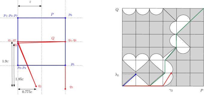
Figure 8. An example in which the greedy algorithm fails to realize the Fréchet matching highlighted in green. Here, $P[1,\gamma_{2}]$ is the longest $\varepsilon$-prefix in $P$ with respect to $Q[1,2]$, as illustrated by the red reachable path. Also $Q[1,\lambda_{2}]$ is the longest $\varepsilon$-prefix in $Q$ with respect to $P[1,2]$ as illustrated by the blue reachable path. Every edge is $2\varepsilon$ long, except for the edges $Q[1,2]$ and $Q[2,3]$ that have lengths $2.02\varepsilon$ and $2.005\varepsilon$, respectively. The latter values are still in the range $[2\varepsilon,(1+\sqrt{2})\varepsilon]$.

4. Optimization and Approximation

In this section, we present two algorithms for computing and approximating the Fréchet distance between two curves with long edges, respectively. First we give an exact algorithm which runs in $O((n+m)\log(n+m))$ time. Afterwards, we present a linear time algorithm which is similar to the greedy decision algorithm, but it uses the notion of minimum prefix to approximate the Fréchet distance.

4.1. Optimization

The main idea of our algorithm is that we compute critical values of the Fréchet distance between two curves and then perform binary search on these to find the optimal value acquired by the decision algorithm. In general, there are a cubic number of critical values, which are candidate values for the Fréchet distance between two polygonal curves. These critical values are those $\varepsilon$ for which $p_{1}\in B(q_{1},\varepsilon)$ or $p_{n}\in B(q_{m},\varepsilon)$, or when decreasing $\varepsilon$ slightly a free space interval disappears on the boundary of a free space cell or a monotone path in the free space becomes non-monotone. See Alt and Godau [2] for more details on critical values. In our case we can show that it suffices to consider only a linear number of critical values, because the assumption on the edge lengths of the curves implies that a piecewise orthogonal matching exists, which reduces the number of possible critical values. Our optimization algorithm consists of the following four steps:

1. Run DecisionAlgorithm($P,Q,\varepsilon_{0}$) with $\varepsilon_{0}=\min\{l_{P}/2,l_{Q}/(1+\sqrt{d})\}$ and store all $\gamma_{i}=\textsc{LongestEpsilonPrefix}(P[\gamma_{i-1},n],Q[i-1,i],\varepsilon_{0})$ for all $i=2,\ldots,m$. Only proceed if DecisionAlgorithm($P,Q,\varepsilon_{0}$) returns “Yes”.

2. If $P[\gamma_{i-1},\gamma_{i}]$ is not $(Q[i-1,i],\varepsilon_{0})$-monotone for some $i=2,\ldots,m$ then return $\delta_{F}(P,Q)=\varepsilon_{0}$.

3. Compute $C:=\cup_{i=2}^{m}C_{i}\cup\{\varepsilon_{0}\}$, where $C_{i}$ is the set of all critical values for $P[\alpha_{i-1},\gamma_{i}]$ and $Q[i-1,i]$. Here, $P(\alpha_{i})$ is the first point along $P[\gamma_{i-1},n]$ that intersects $B(q_{i},\varepsilon_{0})$ and $\alpha_{1}=1$.

4. Sort $C$ and perform binary search on $C$ using DecisionAlgorithm($P,Q,\cdot$) to find $\delta_{F}(P,Q)$.

In step (1) we set $\varepsilon_{0}=\min\{l_{P}/2,l_{Q}/(1+\sqrt{d})\}$. This means that $l_{P}\geq 2\varepsilon_{0}$ and $l_{Q}\geq(1+\sqrt{d})\varepsilon_{0}$. Step (2) handles the case that the matching induced by the $\gamma_{i}$ may not be a piecewise orthogonal matching. But once the algorithm proceeds to step (3), there exists a piecewise orthogonal matching between $P$ and $Q$. This restricts the set of critical values we have to consider in step (3) as follows: Let $\varepsilon^{*}\leq\varepsilon_{0}$ and assume $\varepsilon^{*}=\delta_{F}(P,Q)$. Let $\gamma^{*}_{i}=\textsc{LongestEpsilonPrefix}(P[\gamma^{*}_{i-1},n],Q[i-1,i],\varepsilon^{*})$, for $i=2,\ldots,m$, and let $P(\alpha^{*}_{i})$ be the first intersection point between $P[\gamma^{*}_{i-1},n]$ and $B(q_{i},\varepsilon^{*})$, and $\alpha^{*}_{1}=\gamma^{*}_{1}=1$. From $B(q_{i},\varepsilon^{*})\subseteq B(q_{i},\varepsilon_{0})$ follows that $\alpha_{i}\leq\alpha^{*}_{i}\leq\gamma^{*}_{i}\leq\gamma_{i}$. And since $\gamma_{i-1}\leq\gamma_{i}$, we know that $P[\gamma^{*}_{i-1},\gamma^{*}_{i}]\subseteq P[\alpha_{i-1},\gamma_{i}]$. We thus have observed the following, see Fig. 9:

Observation 4.1.

Let $\varepsilon^{*}\leq\varepsilon_{0}$. For all $i=2,\ldots,m$:

(1) $\alpha_{i}\leq\alpha^{*}_{i}\leq\gamma^{*}_{i}\leq\gamma_{i}$, (2) $P[\gamma^{*}_{i-1},\gamma^{*}_{i}]\subseteq P[\alpha_{i-1},\gamma_{i}]$.

Therefore all critical values for $P[\gamma^{*}_{i-1},\gamma^{*}_{i}]$ and $Q[i-1,i]$ must be contained in the set $C_{i}$ which are the critical values for $P[\alpha_{i-1},\gamma_{i}]$ and $Q[i-1,i]$, and the binary search in step (4) will identify $\varepsilon^{*}$.

Lemma 4.2 (Correctness).

Let $\varepsilon_{0}=\min\{l_{P}/2,l_{Q}/(1+\sqrt{d})\}$ and let $\varepsilon^{*}=\delta_{F}(P,Q)$. If in step (1) of the optimization algorithm DecisionAlgorithm$(P,Q,\varepsilon_{0})$ returns “Yes”, then the optimization algorithm returns $\varepsilon^{*}$ and $\varepsilon^{*}\leq\varepsilon_{0}$. Otherwise $\varepsilon^{*}\geq\varepsilon_{0}$.

Proof 4.3.

If DecisionAlgorithm$(P,Q,\varepsilon_{0})$ returns “No” then Theorem 3.16 implies that $\delta_{F}(P,Q)=\varepsilon^{*}\geq\varepsilon_{0}$. Now suppose, for the remainder of this proof, that DecisionAlgorithm$(P,Q,\varepsilon_{0})$ returns “Yes”. Then we know that all $\gamma_{i}$ exist and $\delta_{F}(P[\gamma_{i-1},\gamma_{i}],Q[i-1,i])\leq\varepsilon_{0}$ for all $i=2,\ldots,m$, and therefore $\varepsilon^{*}\leq\varepsilon_{0}$, see also Theorem 3.16. This implies that $\varepsilon_{0}$ is an upper bound on all critical values in $C$. It remains to show that the optimization algorithm returns $\varepsilon^{*}$.

If in step (2) there is an $i=2,\ldots,m$ such that $P[\gamma_{i-1},\gamma_{i}]$ is not $(Q[i-1,i],\varepsilon)$-monotone, then there must exist an edge $P[j,j+1]$, for $\gamma_{i-1}\leq j<\gamma_{i}$, such that the angle between the direction vectors of $P[j,j+1]$ and $Q[i-1,i]$ is greater than $\pi/2$. The length of all edges in $P$ must be at least $2\varepsilon_{0}$. But for this edge, the only way a (monotone) Fréchet matching between $P[\gamma_{i-1},\gamma_{i}]$ and $Q[i-1,i]$ of width at most $\varepsilon_{0}$ can exist is if $\|p_{j+1}-p_{j}\|=2\varepsilon_{0}$ and both $p_{j}$ and $p_{j+1}$ are matched to $x=B(p_{j},\varepsilon_{0})\cap B(p_{j+1},\varepsilon_{0})\cap Q[i-1,i]$. Therefore the width of such a Fréchet matching is exactly $\varepsilon_{0}$ and $\varepsilon^{*}=\varepsilon_{0}$.

It remains to show that if the algorithm passes step (2) it returns $\varepsilon^{*}$ at the end of step (4). Since $\varepsilon_{0}\in C$ and $\varepsilon^{*}\leq\varepsilon_{0}$, the binary search will return $\varepsilon^{*}$ if $\varepsilon^{*}=\varepsilon_{0}$. So assume now that $\varepsilon^{*}<\varepsilon_{0}$. Since the algorithm passes step (2), it follows from Lemma 3.2 that the matching induced by the $\gamma_{i}$ is indeed a piecewise orthogonal matching of width less than $\varepsilon_{0}$. From Observation 4.1 follows that all critical values for $P[\gamma^{*}_{i-1},\gamma^{*}_{i}]$ and $Q[i-1,i]$ must be contained in the set $C_{i}$ of all critical values for $P[\alpha_{i-1},\gamma_{i}]$ and $Q[i-1,i]$. Thus, $\varepsilon^{*}\in C=\cup_{i=2}^{m}C_{i}$, and the binary search in step (4) returns $\varepsilon^{*}$.

Computing The Critical Values: A piecewise orthogonal matching of width $\varepsilon^{*}$ between $P$ and $Q$ is comprised of orthogonal matchings between $P[\gamma^{*}_{i-1},\gamma^{*}_{i}]$ and $Q[i-1,i]$ for all $i=2,\ldots,m$. The piecewise orthogonal matching may map vertices from $P$ to $Q[i-1,i]$ either by an orthogonal projection or by mapping to the endpoints $q_{i-1},q_{i}$. And vertices $q_{i}$ may be mapped by on orthogonal projection to $P[\alpha_{i},\gamma_{i}]$. These mappings define point-to-point distances that are candidates for $\varepsilon^{*}$, and thus critical values between $P[\gamma^{*}_{i-1},\gamma^{*}_{i}]$ and $Q[i-1,i]$ that we need to optimize over. But since $\varepsilon^{*}$ is not known beforehand, we compute the superset $C_{i}$ of critical values between $P[\alpha_{i-1},\gamma_{i}]$ and $Q[i-1,i]$ as follows: Let ${\cal H}_{1}$ be the hyperplane perpendicular to $Q[i-1,i]$ and tangent to $B(q_{i-1},\varepsilon_{0})$ that intersects $Q[i-1,i]$. Similarly, define ${\cal H}_{2}$ with respect to $B(q_{i},\varepsilon_{0})$. For each $p_{j}\in P[\alpha_{i-1},\gamma_{i}]$: (1) If $p_{j}$ lies between ${\cal H}_{1}$ and ${\cal H}_{2}$, then any orthogonal matching of width $\varepsilon^{*}$ maps $p_{j}$ to its orthogonal projection on $Q[i-1,i]$. We therefore add the distance $\|p_{j},Q[i-1,i]\|$ to $C_{i}$. (2) If $p_{j}$ lies on the $q_{i-1}$-side of ${\cal H}_{1}$, then an orthogonal matching of width $\varepsilon^{*}$ can map $p_{j}$ either to $q_{i-1}$ or to its orthogonal projection on $Q[i-1,i]$. In this case we store both $\|p_{j},Q[i-1,i]\|$ and $\|p_{j}-q_{i-1}\|$ in $C_{i}$. Similarly, if $p_{j}$ lies on the $q_{i}$-side of ${\cal H}_{2}$ then we store $\|p_{j},Q[i-1,i]\|$ and $\|p_{j}-q_{i}\|$ in $C_{i}$. Finally, for each edge $e$ in $P[\alpha_{i},\gamma_{i}]$: (3) we store $\|q_{i},e\|$. See Fig. 9 for more illustration. We have the following theorem:

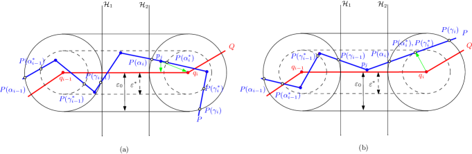
Figure 9. Shown are two examples of orthogonal matchings between $P[\gamma^{*}_{i-1},\gamma^{*}_{i}]$ and $Q[i-1,i]$, and the associated critical values (point-to-point distances defined by the matching). The cylinders $C(Q[i-1,i],\varepsilon_{0})$ and $C(Q[i-1,i],\varepsilon^{*})$ are shown, where $\varepsilon_{0}\geq\varepsilon^{*}$. (a) $p_{j}$ falls into case (2), when the orthogonal matching maps $p_{j}$ either to $q_{i}$ (if $p_{j}$ lies inside $B(q_{i},\varepsilon^{*})$) or orthogonally to $Q[i-1,i]$ (if $p_{j}$ lies outside $B(q_{i},\varepsilon^{*})$). (b) If an edge of $P$ is tangent to $B(q_{i},\varepsilon^{*})$, then case (3) occurs. Here, the orthogonal matching has to map $q_{i}$ to an edge $e$ in $P[\alpha_{i},\gamma_{i}]$.

Theorem 4.4 (Optimization).

Let $P:[1,n]\rightarrow\mathbb{R}^{d}$ and $Q:[1,m]\rightarrow\mathbb{R}^{d}$ be two polygonal curves. If $\delta_{F}(P,Q)<\min\{l_{P}/2,l_{Q}/(1+\sqrt{d})\}$, then $\delta_{F}(P,Q)$ can be computed in $O((n+m)\log(n+m))$ time.

Proof 4.5.

By Lemma 4.2 we know that the optimization algorithm returns $\delta_{F}(P,Q)$ correctly if $\delta_{F}(P,Q)$ is strictly less than $\min\{l_{P}/2,l_{Q}/(1+\sqrt{d})\}$. It only remains to prove the runtime of the algorithm. First we show that the number of critical values is linear. For each segment $Q[i-1,i]$, there are three cases for critical values contained in $C_{i}$: (1) There are at most $\lceil\alpha_{i}-\gamma_{i-1}\rceil+1$ values if vertex $p_{j}$ lies between ${\cal H}_{1}$ and ${\cal H}_{2}$. This is an upper bound for the number of vertices in $P[\gamma_{i-1},\alpha_{i}]$. (2) There are at most $2(\lceil\gamma_{i-1}-\alpha_{i-1}\rceil+1)$ values if vertex $p_{j}$ lies on the $q_{i-1}$-side of ${\cal H}_{1}$, and similarly there are at most $2(\lceil\gamma_{i}-\alpha_{i}\rceil+1)$ values if $p_{j}$ lies on the $q_{i}$-side of ${\cal H}_{2}$. (3) There are at most $\lceil\gamma_{i}-\alpha_{i}\rceil$ critical values for each edge $e$ in $P[\alpha_{i},\gamma_{i}]$. Overall, the total is: $|C_{i}|\leq(\gamma_{i}-\alpha_{i})+(\gamma_{i-1}-\alpha_{i-1})+(\gamma_{i}-\alpha_{i-1})+11<2(\gamma_{i}-\alpha_{i-1})+11=2(\gamma_{i}-\gamma_{i-1})+2(\gamma_{i-1}-\alpha_{i-1})+11$. The latter inequality follows because $\alpha_{i-1}\leq\gamma_{i-1}\leq\alpha_{i}\leq\gamma_{i}$, see Fig. 9. Note that $\sum_{i=2}^{m}(\gamma_{i}-\gamma_{i-1})=\gamma_{m}-\gamma_{1}=n-1$, and $\sum_{i=2}^{m}(\gamma_{i-1}-\alpha_{i-1})<n$, therefore, $|C|=\sum_{i=2}^{m}|C_{i}|<2(n-1)+2n+11(m-1)=O(n+m)$.

The optimization algorithm first runs Algorithm 1 in $O(n+m)$ time, then computes $C$ in $O(n+m)$ time, and finally sorts $C$ in $O((n+m)\log(n+m))$ time and performs binary search on $C$ using the decision algorithm in $O((n+m)\log(n+m))$ time. Therefore, the total runtime is $O((n+m)\log(n+m))$.

4.2. Approximation Algorithm

In this section we present a $\sqrt{d}$-approximation algorithm running in linear time. As a counterpart to the notion of longest $\varepsilon$-prefix we now introduce the notion of minimum prefix, which is the longest prefix of $P$ with minimum Fréchet distance to a line segment $e$.

Definition 4.6 (Minimum Prefix).

Let $P:[1,n]\rightarrow\mathbb{R}^{d}$ be a polygonal curve and $e:[1,2]\rightarrow\mathbb{R}^{d}$ be a segment. Define $\gamma^{\prime}=\max\operatornamewithlimits{argmin}_{1\leq t\leq n}{\delta_{F}(P[1,t],e)}$. We call $P[1,\gamma^{\prime}]$ the minimum prefix of $P$ with respect to $e$.

Note that in the definition above, $P(\gamma^{\prime})$ necessarily lies on the boundary of $B(e_{2},\varepsilon^{\prime})$, where $\varepsilon^{\prime}=\min_{1\leq t\leq n}{\delta_{F}(P[1,t],e)}$. The approximation algorithm is presented in Algorithm 2. First, for an initial threshold $\varepsilon_{0}=\min\{l_{P}/(2\sqrt{d}),l_{Q}/(2d)\}$, it runs the decision algorithm, i.e., DecisionAlgorithm($P,Q,\varepsilon_{0}$). The algorithm only continues if “Yes” gets returned. This ensures that $P$ and $Q$ have long edges, with $l_{P}\geq 2\sqrt{d}\varepsilon>2\varepsilon$ and $l_{Q}\geq 2d\varepsilon>(1+\sqrt{d})\varepsilon$. Then, similar to the decision algorithm, the approximation algorithm greedily searches for longest $\varepsilon$-prefixes with respect to each segment of $Q$. However, it updates the current value of $\varepsilon$ in each step, by computing the minimum prefix and its associated Fréchet distance to the portion of $Q$ considered so far.

1

2ApproximationAlgorithm($P[1,n],Q[1,m]$)

3       $\varepsilon_{0}\leftarrow\min\{l_{P}/2\sqrt{d},l_{Q}/2{d}\}$

4       if DecisionAlgorithm($P,Q,\varepsilon_{0}$)= “No” then  return “I don’t know”

5       $(\gamma_{2},\varepsilon_{2})\leftarrow$MinimumPrefix($P[1,n],Q[1,2]$)

6       $\varepsilon\leftarrow\varepsilon_{2}$

7       $s\leftarrow\gamma_{2}$

8       for $i\leftarrow 3$ to $m$ do

9             $(\gamma_{i},\varepsilon_{i})\leftarrow$MinimumPrefix($P[s,n],Q[i-1,i]$)

10             $\varepsilon\leftarrow\max\{\varepsilon,\varepsilon_{i}\}$

11             $s\leftarrow\gamma_{i}$

12            

13      if $\gamma_{m}=n$ then

14            return $\varepsilon$

15      else

16             $\varepsilon\leftarrow\max\{\varepsilon,\delta_{F}(P[\gamma_{m},n],q_{m})\}$

17             return $\varepsilon$

18      

Algorithm 2 Approximate $\delta_{F}(P,Q)$

Now we are ready to prove the correctness of Algorithm 2:

Lemma 4.7 (The Approximation).

Let $P=P[1,n]$ and $Q=Q[1,m]$ be two polygonal curves and let $\varepsilon^{*}=\delta_{F}(P,Q)$. If $\varepsilon^{*}\leq\min\{l_{P}/2\sqrt{d},l_{Q}/2d\}$ then ApproximationAlgorithm($P,Q$) returns a value between $\varepsilon^{*}$ and $\sqrt{d}\varepsilon^{*}$. Otherwise it returns “I don’t know”.

Proof 4.8.

From Algorithm 2 we have that $\varepsilon_{i}=\delta_{F}(P[\gamma_{i-1},\gamma_{i}],Q[i-1,i])$. We prove by induction on $i$ that $\varepsilon_{i}\leq\sqrt{d}\varepsilon^{*}$. For $i=2$, $\varepsilon_{2}$ is being minimized and obviously $\varepsilon_{2}\leq\varepsilon^{*}<\sqrt{d}\varepsilon^{*}$. For any $i>2$, there are two possible cases: either $\varepsilon_{i}\leq\varepsilon^{*}$ or $\varepsilon_{i}>\varepsilon^{*}$. In the former case, trivially $\varepsilon_{i}<\sqrt{d}\varepsilon^{*}$. In the remainder of the proof we consider the latter case that is $\varepsilon_{i}>\varepsilon^{*}$. We know from Theorem 3.11 that all $\gamma^{*}_{i}=\textsc{LongestEpsilonPrefix}(P[\gamma^{*}_{i-1},n],Q[i-1,i],\varepsilon^{*})$ for all $i=1,2,\ldots,m$ exist. And by inductive hypothesis we know that $\max\{\varepsilon_{2},\ldots,\varepsilon_{i-1}\}\leq\sqrt{d}\varepsilon^{*}$.

We also know from line 8 of Algorithm 2 that $\varepsilon_{i}=\delta_{F}(P[\gamma_{i-1},\gamma_{i}],Q[i-1,i])$ and $P[\gamma_{i-1},\gamma_{i}]$ is the minimum prefix with respect to $Q[i-1,i]$. For the sake of contradiction we assume $\varepsilon_{i}>\sqrt{d}\varepsilon^{*}>\varepsilon^{*}$. We now distinguish two cases:

(a) If $\gamma_{i-1}<\gamma^{*}_{i-1}$, then by Lemma 3.5 we have $\delta_{F}(P[\gamma_{i-1},\gamma^{*}_{i-1}],q_{i-1})\leq\sqrt{d}\varepsilon^{*}$. Also $\delta_{F}(P[\gamma^{*}_{i-1},\gamma^{*}_{i}],Q[i-1,i])\leq\varepsilon^{*}$, hence $\delta_{F}(P[\gamma_{i-1},\gamma^{*}_{i}],Q[i-1,i])\leq\sqrt{d}\varepsilon^{*}<\varepsilon_{i}$. This contradicts the fact that $P[\gamma_{i-1},\gamma_{i}]$ is the minimum prefix of $P[\gamma_{i-1},n]$ with respect to $Q[i-1,i]$, see Fig. 10(a).

(b) Now for the case that $\gamma^{*}_{i-1}<\gamma_{i-1}$, consider the matching $(\sigma,\theta)$ realizing $\delta_{F}(P,Q)=\varepsilon^{*}$. There exists some $t\in[0,1]$ such that $\gamma_{i-1}=\sigma(t)$. We can see that $Q(\theta(t))\in Q[i-1,i]$ as follows: We know that $B(q_{i-1},\varepsilon_{i-1})\cap B(q_{i},\varepsilon^{*})=\emptyset$ since $\|q_{i-1}-q_{i}\|\geq 2d\varepsilon^{*}>(1+\sqrt{d})\varepsilon^{*}$ and $\varepsilon_{i-1}\leq\sqrt{d}\varepsilon^{*}$. This implies $\gamma_{i-1}<\gamma^{*}_{i}$ and therefore $\gamma^{*}_{i-1}<\gamma_{i-1}<\gamma^{*}_{i}$, and correspondingly ${i-1}\leq\theta(t)\leq i$. By inductive hypothesis we know that $\varepsilon_{i-1}=\|q_{i-1}-P(\gamma_{i-1})\|\leq\sqrt{d}\varepsilon^{*}$, thus $Q[i-1,\theta(t)]\subseteq B(P(\gamma_{i-1}),\sqrt{d}\varepsilon^{*})$ which implies $\delta_{F}(P(\gamma_{i-1}),Q[i-1,\theta(t)])\leq\sqrt{d}\varepsilon^{*}$. Combining this with $\delta_{F}(P[\gamma_{i-1},\gamma^{*}_{i}],Q[\theta(t),i])\leq\varepsilon^{*}$ from the optimal matching yields $\delta_{F}(P[\gamma_{i-1},\gamma^{*}_{i}],Q[i-1,i])\leq\sqrt{d}\varepsilon^{*}<\varepsilon_{i}$. This contradicts that $P[\gamma_{i-1},\gamma_{i}]$ is the minimum prefix of $P[\gamma_{i-1},n]$ with respect to $Q[i-1,i]$, see Fig. 10(b).

In the end, if $\gamma_{m}<n=\gamma^{*}_{m}$, then Lemma 3.5 again implies $\delta_{F}(P[\gamma_{m},n],q_{m})\leq\sqrt{d}\varepsilon^{*}$ as claimed. The algorithm returns $\max\{\varepsilon_{2},\ldots,\varepsilon_{m}\}$. Since there has to be some $\varepsilon_{j}>\varepsilon^{*}$, and we proved by induction that all $\varepsilon_{i}\leq\sqrt{d}\varepsilon^{*}$, the algorithm returns a value between $\varepsilon^{*}$ and $\sqrt{d}\varepsilon^{*}$.

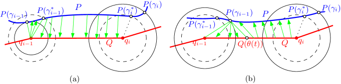
Figure 10. Illustration for the proof of Lemma 4.7 when $\varepsilon_{i}>\varepsilon^{*}$. (a) $\gamma_{i-1}<\gamma^{*}_{i-1}$ (b) $\gamma_{i-1}>\gamma^{*}_{i-1}$.

The MinimumPrefix Procedure: Given a polygonal curve $P:[1,n]\rightarrow\mathbb{R}^{d}$ and a segment $e:[1,2]\rightarrow\mathbb{R}^{d}$, we implement MinimumPrefix($P,e$), as described in Algorithm 3, as follows: For every $i=1,\ldots,n-1$, let $c_{i}$ be the distance associated with a minimum prefix ending on the segment $P[i,i+1]$. Formally, $c_{i}=\min_{t\in[i,i+1]}\delta_{F}(P[1,t],e)$. Algorithm 3 computes all the $c_{i}$ in a dynamic programming fashion. The minimum of the $c_{i}$ is the desired $\varepsilon$, and the LongestEpsilonPrefix computes the corresponding $\gamma$.

1

2MinimumPrefix$(P[1,n],e[1,2])$

3       $c\leftarrow||p_{1}-e_{1}||$

4       $\varepsilon^{\prime}\leftarrow\min\{l_{P}/2,\|e\|/2\sqrt{d}\}$

5       $\gamma^{\prime}\leftarrow\textsc{LongestEpsilonPrefix}(P[1,n],e[1,2],\varepsilon^{\prime})$

6      

7      for $i\leftarrow 1$ to $\lfloor\gamma^{\prime}\rfloor$ do

8             $c_{i}\leftarrow\max\{c,||e_{2},P[i,i+1]||\}$

9             $c\leftarrow\max\{c,||p_{i+1},e[1,2]||\}$

10      $\varepsilon=\min_{1\leq i\leq\lfloor\gamma^{\prime}\rfloor}c_{i}$

11       return $(\varepsilon$, LongestEpsilonPrefix$(P[1,n],e[1,2],\varepsilon))$

Algorithm 3 Compute MinimumPrefix($P[1,n],e[1,2]$)

Before we can prove the correctness of Algorithm 3, we need the following technical lemma that states when $\varepsilon$ is increased, the longest $\varepsilon$-prefix can only get longer.

Lemma 4.9 (Prefix monotonicity).

Let $P:[1,n]\rightarrow\mathbb{R}^{d}$ and $Q:[1,m]\rightarrow\mathbb{R}^{d}$ be two polygonal curves and $\varepsilon>\varepsilon^{\prime}>0$. Let $\gamma_{1}=\gamma^{\prime}_{1}=1$, $\gamma_{i}=\textsc{LongestEpsilonPrefix}(P[\gamma_{i-1},n],Q[i-1,i],\varepsilon)$ and $\gamma_{i}^{\prime}=\textsc{LongestEpsilonPrefix}(P[\gamma^{\prime}_{i-1},n],Q[i-1,i],\varepsilon^{\prime})$ for all $i=2,\ldots,m$. Then $\gamma_{i}<\gamma_{i}^{\prime}$ for all $i=2,\ldots,m$.

Proof 4.10.

The proof is by the induction. For $i=2$, we know that $\delta_{F}(P[1,\gamma^{\prime}_{2}],Q[1,2])\leq\varepsilon^{\prime}<\varepsilon$. Let $x$ be a parameter such that $P(x)$ is the first intersection point between $P[\gamma^{\prime}_{2},n]$ and the boundary of $B(q_{2},\varepsilon)$, thus $\gamma^{\prime}_{2}<x$. Now observe that $\delta_{F}(P[\gamma^{\prime}_{2},x],q_{2})\leq\varepsilon$. Combining $\delta_{F}(P[1,\gamma^{\prime}_{2}],Q[1,2])<\varepsilon$ and $\delta_{F}(P[\gamma^{\prime}_{2},x],q_{2})\leq\varepsilon$ yields $\delta_{F}(P[1,x],Q[1,2])\leq\varepsilon$. Since $\gamma_{2}$ is the longest $\varepsilon$-prefix with respect to $Q[1,2]$, we have $\gamma^{\prime}_{2}<x\leq\gamma_{2}$, and therefore $\gamma^{\prime}_{2}<\gamma_{2}$. Now for $i>2$, by the inductive hypothesis we have $\gamma^{\prime}_{i-1}<\gamma_{i-1}$. It remains to show $\gamma^{\prime}_{i}<\gamma_{i}$. Consider a matching $(\sigma,\theta)$ realizing $\delta_{F}(P[\gamma^{\prime}_{i-1},\gamma^{\prime}_{i}],Q[i-1,i])\leq\varepsilon^{\prime}$. Let $t$ be the value such that $\sigma(t)=\gamma_{i-1}$. Now we construct a new matching for $P[\gamma_{i-1},x]$, where $x$ is defined as in the inductive base, but with respect to $B(q_{i},\varepsilon)$. We know that $\delta_{F}(P(\gamma_{i-1}),Q[i-1,\theta(t)])\leq\varepsilon$. Also we have $\delta_{F}(P[\gamma_{i-1},\gamma^{\prime}_{i}],Q[\theta(t),i])\leq\varepsilon^{\prime}<\varepsilon$ by $(\sigma,\theta)$. Observe that $\delta_{F}(P[\gamma^{\prime}_{i},x],q_{i})\leq\varepsilon$. Thus, $\delta_{F}(P[\gamma_{i-1},x],Q[i-1,i])\leq\varepsilon$ and using a similar argument as in the inductive base we have $\gamma^{\prime}_{i}<x\leq\gamma_{i}$, therefore $\gamma^{\prime}_{i}<\gamma_{i}$.

Now we are ready to prove the correctness of Algorithm 3:

Lemma 4.11 (Correctness).

Let $e:[1,2]\rightarrow\mathbb{R}^{d}$ be a line segment and let $P:[1,n^{\prime}]\rightarrow\mathbb{R}^{d}$ be a polygonal curve monotone with respect to the line supporting $e$. The distance returned by MinimumPrefix$(P,e)$ is $\min_{1\leq t\leq n^{\prime}}{\delta_{F}(P[1,t],e)}$.

Proof 4.12.

According to the algorithm:

$$c_{i}=\max\{\|p_{1}-e_{1}\|,\max_{1\leq j\leq i-1}\|p_{j+1},e\|,\|e_{2},P[i,i+1]\|\}.$$

Since $e[1,2]$ is a segment and $P[1,n^{\prime}]$ is monotone with respect to the line supporting $e$, it follows from Lemma 3.2 that for any $i\leq t\leq i+1$ there exists an orthogonal matching such that:

$$\delta_{F}(P[1,t],e)=\max\{\|p_{1}-e_{1}\|,\max_{1\leq j\leq i-1}\|p_{j+1},e\|,\|P(t)-e_{2}\|\}$$

By taking the minimum on both sides, we get:

$$\min_{i\leq t\leq i+1}\delta_{F}(P[1,t],e)=\max\{\|p_{1}-e_{1}\|,\max_{1\leq j\leq i-1}\|p_{j+1},e\|,\min_{i\leq t\leq i+1}\|P(t)-e_{2}\|\}=c_{i}.$$

It suffices to run the for-loop until $n^{\prime}=\lfloor\gamma^{\prime}\rfloor$, since by the assumption we only compute the minimum $\varepsilon$-prefix $P[1,\gamma]$ if its distance is at most $\varepsilon^{\prime}$ (line 3 of Algorithm 3), and by Lemma 4.9 it follows $\gamma<\gamma^{\prime}$. Therefore, $\varepsilon=\min^{\lfloor\gamma^{\prime}\rfloor}_{i=1}{c_{i}}=\min^{n^{\prime}}_{i=1}{c_{i}}=\min_{1\leq t\leq n^{\prime}}{\delta_{F}(P[1,t],e)}.$

Theorem 4.13 (Runtime).

Let $P:[1,n]\rightarrow\mathbb{R}^{d}$ and $Q:[1,m]\rightarrow\mathbb{R}^{d}$ be two polygonal curves. If $\delta_{F}(P,Q)\leq\min\{l_{P}/(2\sqrt{d}),l_{Q}/(2d)\}$, then Algorithm 2 approximates $\delta_{F}(P,Q)$ in $O(n+m)$ time within an approximation factor of $\sqrt{d}$.

Proof 4.14.

Let $\varepsilon^{*}=\delta_{F}(P,Q)$. The algorithm only proceeds past line 2 if $\varepsilon^{*}\leq\varepsilon_{0}=\min\{l_{P}/2\sqrt{d},l_{Q}/2d\}$ and $\textsc{DecisionAlgorithm}(P,Q,\varepsilon_{0})$ returns “Yes”. Now, let $\varepsilon^{\prime}=\sqrt{d}\varepsilon_{0}$, $\gamma^{\prime}_{1}=1$, and for all $i=2,\ldots,m$ let $\gamma^{\prime}_{i}=\textsc{LongestEpsilonPrefix}(P[\gamma^{\prime}_{i-1},n],Q[i-1,i],\varepsilon^{\prime})$. Note that by definition of $\varepsilon^{\prime}$, both curves have long edges, i.e., $l_{P}\geq 2\sqrt{d}\varepsilon_{0}>2\varepsilon^{\prime}$ and $l_{Q}\geq 2d\varepsilon_{0}=2\sqrt{d}\varepsilon^{\prime}>(1+\sqrt{d})\varepsilon^{\prime}$. From the proof of Lemma 4.7 we know that $\varepsilon_{i}\leq\sqrt{d}\varepsilon^{*}\leq\sqrt{d}\varepsilon_{0}=\varepsilon^{\prime}$ and since $\|q_{i-1}-q_{i}\|>2\sqrt{d}\varepsilon^{\prime}$, we have that $B(q_{i-1},\varepsilon^{\prime})\cap B(q_{i},\varepsilon_{i})=\emptyset$. Therefore, $\gamma^{\prime}_{i-1}<\gamma_{i}$. Lemma 4.9 implies that $\gamma_{i}\leq\gamma^{\prime}_{i}$ due to $\varepsilon_{i}\leq\varepsilon^{\prime}$, therefore $\gamma_{i-1}<\gamma^{\prime}_{i-1}<\gamma_{i}<\gamma^{\prime}_{i}$ for all $i=2,\ldots,m$.

The for-loop in Algorithm 2 has $m-2$ iterations. In iteration $i$, the algorithm calls $\textsc{MinimumPrefix}(P[\gamma_{i-1},\gamma^{\prime}_{i}],Q[i-1,i])$ in line 8. The for-loop in Algorithm 3 has $\lceil\gamma^{\prime}_{i}-\gamma_{i-1}\rceil+1$ iterations, where $\lceil\gamma^{\prime}_{i}-\gamma_{i-1}\rceil+1$ is the upper bound for the number of vertices in $P[\gamma_{i-1},\gamma^{\prime}_{i}]$. Therefore, the runtime of Algorithm 2 is: $\sum_{i=2}^{m}(\lceil\gamma^{\prime}_{i}-\gamma_{i-1}\rceil+1)\leq\sum_{i=2}^{m}({\gamma^{\prime}_{i}-\gamma_{i-1}}+2)=\sum_{i=2}^{m}(\gamma^{\prime}_{i}-\gamma_{i})+\sum_{i=2}^{m}({\gamma_{i}-\gamma_{i-1}})+2(m-1)$. Since $\gamma^{\prime}_{i-1}\leq\gamma_{i}$, we have $\sum_{i=2}^{m}(\gamma^{\prime}_{i}-\gamma_{i})\leq\sum_{i=2}^{m}(\gamma^{\prime}_{i}-\gamma^{\prime}_{i-1})$. Thus, $\sum_{i=2}^{m}(\gamma^{\prime}_{i}-\gamma_{i})+\sum_{i=2}^{m}({\gamma_{i}-\gamma_{i-1}})+2(m-1)\leq\sum_{i=2}^{m}(\gamma^{\prime}_{i}-\gamma^{\prime}_{i-1})+\sum_{i=2}^{m}({\gamma_{i}-\gamma_{i-1}})+2(m-1)=\gamma^{\prime}_{m}-\gamma^{\prime}_{1}+\gamma_{m}-\gamma_{1}+2(m-1)=2(n-1)+2(n-1)+2(m-1)=O(n+m)$.

5. Data Structure For Longest $\varepsilon$-Prefix Queries

In this section, we consider query variants of the setting in Section 3 for curves in the plane. We wish to solve the following problem: Preprocess a polygonal curve $P:[1,n]\rightarrow{\mathbb{R}}^{2}$ into a data structure such that for any polygonal query curve $Q:[1,m]\rightarrow{\mathbb{R}}^{2}$ and a positive $\varepsilon<\min\{l_{P}/2,l_{Q}/(1+\sqrt{2})\}$ one can efficiently decide whether $\delta_{F}(P,Q)\leq\varepsilon$. Note that throughout this section we assume, as before, that $P$ and $Q$ have long edges, i.e., $l_{P}>2\varepsilon$ and $l_{Q}>(1+\sqrt{2})\varepsilon$. Our query algorithm is identical to Algorithm 1. However, the key idea for speeding up the query algorithm is to efficiently compute $\textsc{LongestEpsilonPrefix}(P[1,n],Q[1,2],\varepsilon)$ for a given query segment $Q[1,2]$ in sublinear time. Our algorithm to compute the longest $\varepsilon$-prefix with respect to $Q[1,2]$ is shown in Algorithm 4. According to Lemma 3.2 if $\delta(P[1,\gamma],Q[1,2])\leq\varepsilon$, then $P[1,\gamma]$ is $(Q[1,2],\varepsilon)$-monotone. This is equivalent to computing the largest parameter $1<t\leq n$ such that the following conditions hold: (1) $p_{1}\in B(q_{1},\varepsilon)$ and $P(t)\in B(q_{2},\varepsilon)$, (2) $P[1,t]\subseteq C(Q[1,2],\varepsilon)$, and (3) $P[1,t]$ is monotone with respect to line supporting $Q[1,2]$. Note that the smallest value $t$ that violates either of the conditions above is a potential $\gamma$.

1

2 LongestEpsilonPrefix$(P[1,n],Q[1,2],\varepsilon)$

3      

4      if $p_{1}\notin B(q_{1},\varepsilon)$ then return ‘null’

5       $\lambda\leftarrow$ LongestMonotonePrefix($P[1,n],Q[1,2]$)

6      

7      $\alpha\leftarrow$ FirstIntersection($P[1,\lambda],B(q_{2},\varepsilon))$

8      

9      if $\alpha=null$ then return ‘null’

10      

11      $\beta\leftarrow$ LastIntersection($P[1,\lambda],B(q_{2},\varepsilon))$

12      

13      $r\leftarrow$ CylinderIntersection($P[1,\lambda],C(Q[1,2],\varepsilon)$)

14      

15      if $r=null$ then return $\min(\lambda,\beta)$

16      

17      if $r<\alpha$ or $\lambda<\alpha$ then return ‘null’

18      

19      if $\alpha<r<\beta$ or $\alpha<\lambda<\beta$ then return $\min(r,\lambda)$

20      

21      if $r>\beta$ and $\lambda>\beta$ then return $\beta$

22      

Algorithm 4 Compute LongestEpsilonPrefix($P[1,n],Q[1,2],\varepsilon$)

Here, LongestMonotonePrefix returns $\lambda$, where $P(\lambda)$ is the endpoint of the longest subcurve of $P[1,n]$ that starts in $p_{1}$ and is monotone with respect to the line supporting $Q[1,2]$. FirstIntersection returns $\alpha$, where $P(\alpha)$ is the first intersection point between $P[1,\lambda]$ and $B(q_{2},\varepsilon)$. Similarly, LastIntersection returns $\beta$, where $P(\beta)$ is the last intersection point. CylinderIntersection finds $r$ where $P(r)$ is the first point along $P$ that intersects the boundary of $C(Q[1,2],\varepsilon)$.

Computing LongestMonotonePrefix: We store all the edges of $P$ in the leaves of a binary tree $T$ ordered with respect to their indices. We call the subset of edges stored in the leaves of the subtree rooted at a node $v$ the canonical subset of $v$. A set of nodes $v_{1},\cdots,v_{k}$ in the subtree of $v$ is called a set of canonical nodes of $v$ if their leaves sets are disjoint and the union of their leaves sets is the leaves of the subtree of $v$. For each edge in $P$ we consider its direction vector. Each internal node $v$ stores the pair of the minimum/maximum angles between the direction vector and $x$-axis among all associated direction vectors stored in its canonical subset. Once given a query angle $\Phi$ and a starting point $p_{1}$, we retrieve $O(\log n)$ many leftmost (starting with $p_{1}$) canonical nodes of $T$ whose leaves spans all edges in $P$ that satisfy the monotonicity condition, i.e., condition (3) as mentioned earlier, with respect to $\Phi$. This can simply be done by recursively searching children of a node $v$ violating the monotonicity condition with respect to $\Phi$. Once satisfying the condition, we already have $O(\log n)$ internal nodes to report their leaves as $P[1,\lambda]$. Searching children and reporting nodes take $O(\log n)$ time altogether using $O(n)$ space and $O(n\log n)$ preprocessing time.

Computing FirstIntersection and LastIntersection: Let ${\cal H}$ be the hyperplane intersecting $Q[1,2]$ that is perpendicular to $Q[1,2]$ and is tangent to $B(q_{2},\varepsilon)$. Let ${\cal H}^{\prime}$ be the other hyperplane perpendicular to $Q[1,2]$ and tangent to $B(q_{2},\varepsilon)$. Since $P[1,\lambda]$ is monotone with respect to the line supporting $Q[1,2]$, we know that $\lambda$ must lie on the $q_{2}$-side of ${\cal H}$. And $P(\alpha)\in P[1,\lambda]$ must be located on the first edge intersecting ${\cal H}_{2}$. We start from $p_{1}$ and perform an exponential search on the edges of $P[1,\lambda]$ to find the first edge that intersects ${\cal H}$. Once the edge is found, we can find $P(\alpha)$ in constant time since each edge of $P$ is longer than $2\varepsilon$ which is the diameter of $B(q_{2},\varepsilon)$. Using the same method we can find $P(\beta)\in P[1,\lambda]$, if we consider ${\cal H}^{\prime}$ instead of ${\cal H}$. If $\lambda$ is on the $q_{2}$-side of ${\cal H}^{\prime}$, we perform the exponential search on $P[1,\lambda]$ to find $P(\beta)$. If $\lambda$ is on the $q_{1}$-side of ${\cal H}^{\prime}$ then there is no $P(\beta)\in P[1,\lambda]$ and the algorithm does not require it. The whole process takes $O(\log n)$ time.

Computing CylinderIntersection: Similar to Gudmundsson and Smid [16], we construct a balanced binary search tree storing the points $p_{1},p_{2},\ldots,p_{n}$ in its leaves (sorted by their indices). At each node of this tree, we store the convex hull of all points stored in its subtree. Given a query range $P[1,\lambda]$, we can retrieve $O(\log n)$ many canonical nodes of the tree containing convex hulls whose leaves span the whole range. For each convex hull we only need to compute extreme points with respect to the direction vector of the edge $Q[1,2]$. If all extreme points lie inside $C(Q[1,2],\varepsilon)$, then $r=null$, otherwise we consider the first extreme point $P(x)$ of some convex hull which lies outside $C(Q[1,2],\varepsilon)$. Note that $P[1,x]$ crosses one of the two boundaries of $C(Q[1,2],\varepsilon)$. Performing exponential search on $P[1,x]$ will find the first point that lies outside the respective boundary of $C(Q[1,2],\varepsilon)$ for which $P(x)$ is obtained. This structure needs $O(n\log n)$ space and preproccessing time and answers queries in $O(\log^{2}n)$ time. Plugging Algorithm 4 into the decision algorithm (Algorithm 1), we obtain the following theorem:

Theorem 5.1 (General Curves).

Let $P:[1,n]\rightarrow{\mathbb{R}}^{2}$ be a polygonal curve. A data structure of $O(n\log n)$ size can be built in $O(n\log n)$ time such that for any query curve $Q:[1,m]\rightarrow{\mathbb{R}}^{2}$ and a positive constant $\varepsilon<\min(l_{P}/2,l_{Q}/(1+\sqrt{2}))$, it can be decided in $O(m\log^{2}n)$ time whether $\delta_{F}(P,Q)\leq\varepsilon$.

Proof 5.2.

The correctness of the query algorithm follows from Theorem 3.11. As we mentioned, the space and preprocessing time of the whole data structure is $O(n\log n)$. Using Algorithm 4, the longest $\varepsilon$-prefix can be computed in $O(\log^{2}n)$ time per segment, and hence the query algorithm runs in $O(m\log^{2}n)$ time.

When $P$ is an $x$-monotone curve, we can handle queries in a slightly faster query time and also smaller space. In this case, we assume that $\varepsilon$ is given at the preprocessing stage. The $x$-monotonicity of $P$ allows us to use a different data structure for supporting the CylinderIntersection procedure, since the query time and space of this structure dominates the cost of our entire data structure.

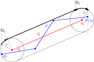
Figure 11. Illustrating how combining the straight and circular line ray shooting queries can find the first point along $P[1,\lambda]$ that leaves $C(Q[1,2],\varepsilon)$.

We implement the CylinderIntersection procedure by performing two types of ray shooting queries, straight and circular, along the boundary of $C(Q[1,2],\varepsilon)$. It is easy to see that it suffices to perform at most two straight ray shooting queries and four circular ray shooting queries since $P$ is $x$-monotone. See Fig. 11 for an illustration of the queries for the top part of the boundary of $C(Q[1,2],\varepsilon)$.

For straight ray shooting queries we use the data structure by Hershberger and Suri [18]. Given a simple polygon, their structure returns the first point on the boundary of the polygon that is hit by a query ray $\rho$. It can be built in $O(n\log n)$ time using $O(n)$ space and answer queries in $O(\log n)$ time. However, to be able to use this structure we need to reduce our problem to ray shooting in a simple polygon. Let $P_{H}$ be the (unbounded) polygon bounded from below by $P$, from the left by a vertical ray from $p_{1}$ to $\infty$, and from the right by a vertical ray from $p_{n}$ to $\infty$. Similarly let $P_{L}$ be the (unbounded) polygon bounded from above by $P$, from the left by a vertical ray from $p_{1}$ to $-\infty$, and from the right by a vertical ray from $p_{n}$ to $-\infty$. We build one data structure for $P_{L}$ and one for $P_{H}$. For circular ray shooting queries we use the data structure by Cheong et al. [9]. Consider a simple polygon ${\cal P}$ with size $n$ in the plane and let $r>0$. For any circular query ray $\rho$ with center $o$, radius $r$, and start point $s^{\prime}$, one can report in $O(\log n)$ query time the first point on the boundary of ${\cal P}$ which is hit by $\rho$. Combining these structures gives us the first point along $P[1,\lambda]$ that leaves the cylinder, which completes the implementation of CylinderIntersection. We have the following theorem:

Theorem 5.3 ($x$-Monotone Preprocessed Curve).

Let $\varepsilon>0$ and let $P:[1,n]\rightarrow{\mathbb{R}}^{2}$ be an $x$-monotone polygonal curve in ${\mathbb{R}}^{2}$ such that $l_{P}>2\varepsilon$. A linear size data structure can be built in $O(n\log n)$ time such that for any polygonal query curve $Q:[1,m]\rightarrow{\mathbb{R}}^{2}$ with $l_{Q}>(1+\sqrt{2})\varepsilon$, one can decide in $O(m\log n)$ time whether $\delta_{F}(P,Q)\leq\varepsilon$.

6. Discussion and Future Work

In this paper we provided a linear time decision algorithm, an $O((n+m)\log(n+m))$ time optimization algorithm, a linear time $\sqrt{d}$-approximation algorithm and a data structure with $O(m\log^{2}n)$ query time for the Fréchet distance between curves that have long edges. Our algorithms are simple greedy algorithms that run in any constant dimension. In Section 3.4 we gave a critical example that justifies our assumptions on the edge lengths.

We proposed several greedy algorithms. Our assumption on the edge lengths allowed us to obtain a linear time constant-factor approximation algorithm for the (continuous) Fréchet distance. On the other hand, Bringmann and Mulzer [6] presented a greedy linear time exponential approximation algorithm for general curves under the discrete Fréchet distance. An interesting future research direction would be to develop a trade-off between the lengths of edges and the runtime, and in general prove hardness in terms of the edge lengths.

Acknowledgements.

We thank the anonymous reviewers for helping to improve the presentation of this paper. We particularly thank one anonymous reviewer for insightful comments that helped us to improve the algorithm in Section 3.

References

- [1] P.K. Agarwal, R.B. Avraham, H. Kaplan and M. Sharir, Computing the discrete Fréchet distance in subquadratic time, SIAM Journal on Computing 43 (2014) 429–449.
- [2] H. Alt and M. Godau, Computing the Fréchet distance between two polygonal curves, International Journal of Computational Geometry and Applications 5(1–2) (1995) 75–91.
- [3] H. Alt, C. Knauer and C. Wenk, Comparison of distance measures for planar curves, Algorithmica 38(2) (2004) 45–58.
- [4] B. Aronov, S. Har-Peled, C. Knauer, Y. Wang and C. Wenk, Fréchet distance for curves, Revisited, 14th Annual European Symposium on Algorithms (2006) pp. 52–63.
- [5] K. Bringmann, Why walking the dog takes time: Fréchet distance has no strongly subquadratic algorithms unless SETH fails, Proceedings of the 55th IEEE Symposium on Foundations of Computer Science (FOCS) (2014) pp. 661–670.
- [6] K. Bringmann and W. Mulzer, Approximability of the discrete Fréchet distance, Journal of Computational Geometry 7(2) (2016) 46–76.
- [7] K. Buchin, M.Buchin, C. Knauer, G. Rote and C. Wenk, How difficult is it to walk the dog?, 23rd European Workshop on Computational Geometry (2007) pp. 170–173.
- [8] K. Buchin, M. Buchin, W. Meulemans and W. Mulzer, Four Soviets walk the dog - with an application to Alt’s conjecture, Discrete & Computational Geometry 58(1) (2017) 180–216.
- [9] S.-W. Cheng, O. Cheong, H. Everett and R. van Oostrum, Hierarchical decompositions and circular ray shooting in simple polygons, Discrete & Computational Geometry 32(3) (2002) 401–415.
- [10] A. Driemel and S. Har-Peled, Jaywalking your dog: computing the Fréchet distance with shortcuts, SIAM Journal on Computing 42 (2013) 1830–1866.
- [11] A. Driemel, S. Har-Peled and C. Wenk, Approximating the Fréchet distance for realistic curves in near linear time, Discrete & Computational Geometry 48 (2012) 94–127.
- [12] A. Efrat, L.J. Guibas, S. Har-Peled, J.S.B. Mitchell and T.M Murali, New similarity measures between polylines with applications to morphing and polygon sweeping, Discrete & Computational Geometry 28(4) (2002) 535–569.
- [13] J. Gudmundsson, P. Laube and T. Wolle, Movement patterns in spatio-temporal data, Encyclopedia of GIS (Springer-Verlag, 2007).
- [14] J. Gudmundsson, M. Mirzanezhad, A. Mohades and C. Wenk, Fast Fréchet distance between curves with long edges, arXiv e-prints (1710.10521, Oct. 2017).
- [15] J. Gudmundsson, M. Mirzanezhad, A. Mohades and C. Wenk, Fast Fréchet distance between curves with long edges, Proceedings of the 3rd International Workshop on Interactive and Spatial Computing (IWISC) (2018) pp. 52–58.
- [16] J. Gudmundsson and M. Smid, Fréchet queries in geometric trees, 21st European Symposium on Algorithms (ESA) (2013) pp. 565–576.
- [17] J. Gudmundsson and M. Smid, Fast algorithms for approximate Fréchet matching queries in geometric trees, Computational Geometry – Theory and Applications 48(6) (2015) 479–494.
- [18] J. Hershberger and S. Suri, A pedestrian approach to ray shooting: shoot a ray, take a walk, Journal of Algorithms 18(3) (1995) 403–431.
- [19] M. Jiang, Y. Xu and B. Zhu, Protein structure-structure alignment with discrete Fréchet distance, Journal of Bioinformatics and Computational Biology 6(1) (2008) 51–64.
- [20] North America Migration Flyways, https://www.nps.gov/pais/learn/nature/birds.htm, Accessed: 2016-09-21.
- [21] R. Sriraghavendra, K. Karthik and C. Bhattacharyya, Fréchet distance based approach for searching online handwritten documents, Proc. 9th International Conference on Document Analysis and Recognition (ICDAR) (2007) pp. 461–465.