Online Approximate Optimal Station Keeping of a Marine Craft in the Presence of a Current

Abstract

Online approximation of the optimal station keeping strategy for a fully actuated six degrees-of-freedom marine craft subject to an irrotational ocean current is considered. An approximate solution to the optimal control problem is obtained using an adaptive dynamic programming technique. The hydrodynamic drift dynamics of the dynamic model are assumed to be unknown; therefore, a concurrent learning-based system identifier is developed to identify the unknown model parameters. The identified model is used to implement an adaptive model-based reinforcement learning technique to estimate the unknown value function. The developed policy guarantees uniformly ultimately bounded convergence of the vehicle to the desired station and uniformly ultimately bounded convergence of the approximated policies to the optimal polices without the requirement of persistence of excitation. The developed strategy is validated using an autonomous underwater vehicle, where the three degrees-of-freedom in the horizontal plane are regulated. The experiments are conducted in a second-magnitude spring located in central Florida.

I Introduction

Marine craft, which include ships, floating platforms, autonomous underwater vehicles (AUV), etc, play a vital role in commercial, military and recreational objectives. Marine craft are often required to remain on a station for an extended period of time, e.g., floating oil platforms, support vessels, and AUVs acting as a communication link for multiple vehicles or persistent environmental monitors. The success of the vehicle often relies on the vehicle’s ability to hold a precise station (e.g., station keeping near structures or underwater features). The cost of holding that station is correlated to the energy expended for propulsion through consumption of fuel and wear on mechanical systems, especially when station keeping in environments with a persistent current. Therefore, by reducing the energy expended for station keeping objectives, the cost of holding a station can be reduced.

Precise station keeping of a marine craft is challenging because of nonlinearities in the dynamics of the vehicle. A survey of station keeping for surface vessels can be found in [1]. Common approaches employed to control a marine craft include robust and adaptive control methods [2, 3, 4, 5]. These methods provide robustness to disturbances and/or model uncertainty; however, they do not explicitly account for the cost of the control effort. Motivated by the desire to balance energy expenditure and the accuracy of the vehicle’s station, approximate optimal control methods are examined in this paper to minimize a user defined cost function of the total control effort (energy expended) and state error (station accuracy). Because of the difficulties associated with finding closedform analytical solutions to optimal control problems for marine craft, efforts such as [6] numerically approximate the solution to the Hamilton-Jacobi-Bellman (HJB) equation using an iterative application of Galerkin’s method.

Various methods have been proposed to find an approximate solution to the HJB equation. Adaptive dynamic programming (ADP) is one such method where a solution to the HJB equation is approximated using parametric function approximation techniques. ADP-based techniques have been used to approximate optimal control policies for regulation (e.g., [7, 8, 9, 10, 11]) of general nonlinear systems. Efforts in [12] and [13] present ADP-based solutions to the Hamilton-Jacobi-Isaacs equation that yield an approximate optimal policy accounting for state-dependent disturbances. However, these methods do not consider explicit time-varying disturbances such as the dynamics that are introduced due to the presence of current.

In this result, an optimal station keeping policy that captures the desire to balance the need to accurately hold a station and the cost of holding that station through a quadratic performance criterion is generated for a fully actuated marine craft. The developed controller differs from results such as [7] and [8] in that it tackles the challenges associated with the introduction of a time-varying irrotational current. Since the hydrodynamic parameters of a marine craft are often difficult to determine, a concurrent learning system identifier is developed. As outlined in [14], concurrent learning uses additional information from recorded data to remove the persistence of excitation requirement associated with traditional system identifiers. The proposed model-based ADP method generates the optimal station keeping policy using a combination of on-policy and off-policy data, eliminating the need for physical exploration of the state space. A Lyapunov-based stability analysis is presented which guarantees uniformly ultimately bounded (UUB) convergence of the marine craft to its station and UUB convergence of the approximated policy to the optimal policy.

To illustrate the performance of the developed controller, an AUV is used to collect experimental data. Specifically, the developed strategy is implemented for planar regulation of an AUV near the vent of a second-magnitude spring located in central Florida. The experimental results demonstrate the developed method’s ability to simultaneously identify the unknown hydrodynamic parameters and generate an approximate optimal policy using the identified model in the presence of a current.

II Vehicle Model

Consider the nonlinear equations of motion for a marine craft including the effects of irrotational ocean current given in Section 7.5 of [15] as

$$\dot{\eta}=J_{E}\left(\eta\right)\nu,$$ (1)

$$M_{RB}\dot{\nu}+C_{RB}\left(\nu\right)\nu+M_{A}\dot{\nu}_{r}+C_{A}\left(\nu_{r}\right)\nu_{r}$$

$$+D_{A}\left(\nu_{r}\right)\nu_{r}+G\left(\eta\right) = \tau_{b}$$ (2)

where $\nu\in\mathbb{R}^{n}$ is the body-fixed translational and angular velocity vector, $\nu_{c}\in\mathbb{R}^{n}$ is the body-fixed irrotational current velocity vector, $\nu_{r}=\nu-\nu_{c}$ is the relative body-fixed translational and angular fluid velocity vector, $\eta\in\mathbb{R}^{n}$ is the earth-fixed position and orientation vector, $J_{E}:\mathbb{R}^{n}\rightarrow\mathbb{R}^{n\times n}$ is the coordinate transformation between the body-fixed and earth-fixed coordinates, $M_{RB}\in\mathbb{R}^{n\times n}$ is the constant rigid body inertia matrix, $C_{RB}:\mathbb{R}^{n}\rightarrow\mathbb{R}^{n\times n}$ is the rigid body centripetal and Coriolis matrix, $M_{A}\in\mathbb{R}^{n\times n}$ is the constant hydrodynamic added mass matrix, $C_{A}:\mathbb{R}^{n}\rightarrow\mathbb{R}^{n\times n}$ is the unknown hydrodynamic centripetal and Coriolis matrix, $D_{A}:\mathbb{R}^{n}\rightarrow\mathbb{R}^{n\times n}$ is the unknown hydrodynamic damping and friction matrix, $G:\mathbb{R}^{n}\rightarrow\mathbb{R}^{n}$ is the gravitational and buoyancy force and moment vector, and $\tau_{b}\in\mathbb{R}^{n}$ is the body-fixed force and moment control input.

In the case of a three degree-of-freedom (DOF) planar model with orientation represented as Euler angles, the state vectors in $\eqref{eq:kinematics}$ and (2) are further defined as

$$\eta\triangleq\left[\begin{array}[]{ccc}x&y&\psi\end{array}\right]^{T},$$

$$\nu\triangleq\left[\begin{array}[]{ccc}u&v&r\end{array}\right]^{T},$$

where $x$, $y\in\mathbb{R}$, are the earth-fixed position vector components of the center of mass, $\psi\in\mathbb{R}$ represents the yaw angle, $u$, $v\in\mathbb{R}$ are the body-fixed translational velocities, and $r\in\mathbb{R}$ is the body-fixed angular velocity. The irrotational current vector is defined as

$$\nu_{c}\triangleq\left[\begin{array}[]{ccc}u_{c}&v_{c}&0\end{array}\right]^{T},$$

where $u_{c}$, $v_{c}\in\mathbb{R}$ are the body-fixed current translational velocities. The coordinate transformation $J_{E}\left(\eta\right)$ is given as

$$J_{E}\left(\eta\right)=\left[\begin{array}[]{ccc}\cos\left(\psi\right)&-\sin\left(\psi\right)&0\\ \sin\left(\psi\right)&\cos\left(\psi\right)&0\\ 0&0&1\end{array}\right].$$

Assumption 1.

The marine craft is neutrally buoyant if submerged and the center of gravity is located vertically below the center of buoyancy on the $z$ axis if the vehicle model includes roll and pitch.

III System Identifier

Since the hydrodynamic effects pertaining to a specific marine craft may be unknown, an online system identifier is developed for the vehicle drift dynamics. Consider the control affine form of the vehicle model,

$$\dot{\zeta}=Y\left(\zeta,\nu_{c}\right)\theta+f_{0}\left(\zeta,\dot{\nu}_{c}\right)+g\tau_{b},$$ (3)

where $\zeta\triangleq\left[\begin{array}[]{cc}\eta&\nu\end{array}\right]^{T}\in\mathbb{R}^{2n}$ is the state vector. The unknown hydrodynamics are linear-in-the-parameters with $p$ unknown parameters where $Y:\mathbb{R}^{2n}\times\mathbb{R}^{n}\rightarrow\mathbb{R}^{2n\times p}$ is the regression matrix and $\theta\in\mathbb{R}^{p}$ is the vector of unknown parameters. The unknown hydrodynamic effects are modeled as

$$Y\left(\zeta,\nu_{c}\right)\theta=\left[\begin{array}[]{c}0\\ -M^{-1}C_{A}\left(\nu_{r}\right)\nu_{r}-M^{-1}D_{A}\left(\nu_{r}\right)\nu_{r}\end{array}\right],$$

and known rigid body drift dynamics $f_{0}:\mathbb{R}^{2n}\times\mathbb{R}^{n}\rightarrow\mathbb{R}^{2n}$ are modeled as

$$f_{0}\left(\zeta,\dot{\nu}_{c}\right)=\\ \left[\begin{array}[]{c}J_{E}\left(\eta\right)\nu\\ M^{-1}M_{A}\dot{\nu}_{c}-M^{-1}C_{RB}\left(\nu\right)\nu-M^{-1}G\left(\eta\right)\end{array}\right],$$

where $M\triangleq M_{RB}+M_{A}$, and the body-fixed current velocity $\nu_{c}$, and acceleration $\dot{\nu}_{c}$ are assumed to be measurable. The known constant control effectiveness matrix $g\in\mathbb{R}^{2n\times n}$ is defined as

$$g\triangleq\left[\begin{array}[]{c}0\\ M^{-1}\end{array}\right].$$

An identifier is designed as

$$\dot{\hat{\zeta}}=Y\left(\zeta,\nu_{c}\right)\hat{\theta}+f_{0}\left(\zeta,\dot{\nu}_{c}\right)+g\tau_{b}+k_{\zeta}\tilde{\zeta},$$ (4)

where $\tilde{\zeta}\triangleq\zeta-\hat{\zeta}$ is the measurable state estimation error, and $k_{\zeta}\in\mathbb{R}^{2n\times 2n}$ is a constant positive definite, diagonal gain matrix. Subtracting (4) from (3), yields

$$\dot{\tilde{\zeta}}=Y\left(\zeta,\nu_{c}\right)\tilde{\theta}-k_{\zeta}\tilde{\zeta},$$

where $\tilde{\theta}\triangleq\theta-\hat{\theta}$ is the parameter identification error.

III-A Parameter Update

Traditional adaptive control techniques require persistence of excitation to ensure the parameter estimates $\hat{\theta}$ converge to their true values $\theta$ (cf. [16] and [17]). Persistence of excitation often requires an excitation signal to be applied to the vehicle’s input resulting in unwanted deviations in the vehicle state. These deviations are often in opposition to the vehicle’s control objectives. Alternatively, a concurrent learning-based system identifier can be developed (cf. [14] and [18]). The concurrent learning-based system identifier relaxes the persistence of excitation requirement through the use of a prerecorded history stack of state-action pairs.

Assumption 2.

There exists a prerecorded data set of sampled data points $\left\{\zeta_{j},\nu_{cj},\dot{\nu}_{cj},\tau_{bj}\in\chi|j=1,2,\ldots,M\right\}$ with a numerically calculated state derivatives $\dot{\bar{\zeta}}_{j}$ at each recorded state-action pair such that $\forall t\in\left[0,\infty\right)$,

$$\mathrm{rank}\left(\sum_{j=1}^{M}Y_{j}^{T}Y_{j}\right)=p,$$ (5)

$$\left\|\dot{\bar{\zeta}}_{j}-\dot{\zeta}_{j}\right\|<\bar{d},\forall j,$$

where $Y_{j}\triangleq Y\left(\zeta_{j},\nu_{cj}\right)$, $f_{0j}\triangleq f_{0}\left(\zeta_{j}\right)$, $\dot{\zeta}_{j}=Y_{j}\theta+f_{0j}+g\tau_{bj}$, and $\bar{d}\in\left[0,\infty\right)$ is a constant.

The parameter estimate update law is given as

$$\dot{\hat{\theta}}=\Gamma_{\theta}Y\left(\zeta,\nu_{c}\right)^{T}\tilde{\zeta}+\Gamma_{\theta}k_{\theta}\sum_{j=1}^{M}Y_{j}^{T}\left(\dot{\bar{\zeta}}_{j}-f_{0j}-g\tau_{bj}-Y_{j}\hat{\theta}\right),$$ (6)

where $\Gamma_{\theta}$ is a positive definite, diagonal gain matrix, and $k_{\theta}$ is a positive, scalar gain matrix. To facilitate the stability analysis, the parameter estimate update law is expressed in the advantageous form

$$\dot{\hat{\theta}}=\Gamma_{\theta}Y\left(\zeta,\nu_{c}\right)^{T}\tilde{\zeta}+\Gamma_{\theta}k_{\theta}\sum_{j=1}^{M}Y_{j}^{T}\left(Y_{j}\tilde{\theta}+d_{j}\right),$$

where $d_{j}=\dot{\bar{\zeta}}_{j}-\dot{\zeta}_{j}$.

Remark 1.

The update law in (6) does not require instantaneous measurement of acceleration. Acceleration only needs to be computed at the past time instances when the data points $\left(\zeta_{j},\nu_{cj},\dot{\nu}_{cj},\tau_{bj}\right)$ were recorded. Acceleration at a past time instance $t^{*}$ can be accurately computed by recording position and velocity signals over a time interval that contains $t^{*}$ in its interior and using noncausal estimation methods such as optimal fixed-point smoothing [20, p. 170].

III-B Convergence Analysis

Consider the candidate Lyapunov function $V_{P}:\mathbb{R}^{2n+p}\times\left[0,\infty\right)$ given as

$$V_{P}\left(Z_{P}\right)=\frac{1}{2}\tilde{\zeta}^{T}\tilde{\zeta}+\frac{1}{2}\tilde{\theta}^{T}\Gamma_{\theta}^{-1}\tilde{\theta},$$ (7)

where $Z_{P}\triangleq\left[\begin{array}[]{cc}\tilde{\zeta}^{T}&\tilde{\theta}^{T}\end{array}\right]$. The candidate Lyapunov function can be bounded as

$$\frac{1}{2}\min\left\{1,\underline{\gamma_{\theta}}\right\}\left\|Z_{P}\right\|^{2}\leq V_{P}\left(Z_{P}\right)\leq\frac{1}{2}\max\left\{1,\overline{\gamma_{\theta}}\right\}\left\|Z_{P}\right\|^{2}$$ (8)

where $\underline{\gamma_{\theta}},\overline{\gamma_{\theta}}$ are the minimum and maximum eigenvalues of $\Gamma_{\theta}$, respectively.

The time derivative of the candidate Lyapunov function in (7) is

$$\dot{V}_{P}=-\tilde{\zeta}^{T}k_{\zeta}\tilde{\zeta}-k_{\theta}\tilde{\theta}^{T}\sum_{j=1}^{M}Y_{j}^{T}Y_{j}\tilde{\theta}-k_{\theta}\tilde{\theta}^{T}\sum_{j=1}^{M}Y_{j}^{T}d_{j}.$$

The time derivative may be upper bounded by

$$\dot{V}_{P}\leq-\underline{k_{\zeta}}\left\|\tilde{\zeta}\right\|^{2}-k_{\theta}\underline{y}\left\|\tilde{\theta}\right\|^{2}+k_{\theta}d_{\theta}\left\|\tilde{\theta}\right\|,$$ (9)

where $\underline{k_{\zeta}},\underline{y}$ are the minimum eigenvalues of $k_{\zeta}$ and $\sum_{j=1}^{M}Y_{j}^{T}Y_{j}$, respectively, and $d_{\theta}=\bar{d}\sum_{j=1}^{M}\left\|Y_{j}\right\|$. Completing the squares, (9) may be upper bounded by

$$\dot{V}_{P}\leq-\underline{k_{\zeta}}\left\|\tilde{\zeta}\right\|^{2}-\frac{k_{\theta}\underline{y}}{2}\left\|\tilde{\theta}\right\|^{2}+\frac{k_{\theta}d_{\theta}^{2}}{2\underline{y}},$$

which may be further upper bounded by

$$\dot{V}_{P}\leq-\alpha_{P}\left\|Z_{P}\right\|^{2},\forall\left\|Z_{P}\right\|\geq K_{P}>0,$$ (10)

where $\alpha_{P}\triangleq\frac{1}{2}\min\left\{2\underline{k_{\zeta}},k_{\theta}\underline{y}\right\}$ and $K_{P}\triangleq\sqrt{\frac{k_{\theta}d_{\theta}^{2}}{2\alpha_{P}\underline{y}}}$. Using (8) and (10), $\tilde{\zeta}$ and $\tilde{\theta}$ can be shown to exponentially decay to a ultimate bound as $t\rightarrow\infty$. The ultimate bound may be made arbitrarily small depending on the selection of the gains $k_{\zeta}$ and $k_{\theta}$.

IV Problem Formulation

IV-A Residual Model

The presence of a time-varying irrotational current yields unique challenges in the formulation of the optimal regulation problem. Since the current renders the system non-autonomous, a residual model that does not include the effects of the irrotational current is introduced. The residual model is used in the development of the optimal control problem in place of the original model. A disadvantage of this approach is that the optimal policy is developed for the current-free model. In the case where the earth-fixed current is constant, the effects of the current may be included in the development of the optimal control problem as detailed in Appendix A.

The residual model can be written in a control affine form as

$$\dot{\zeta}=Y_{res}\left(\zeta\right)\theta+f_{0_{res}}\left(\zeta\right)+gu,$$ (11)

where the unknown hydrodynamics are linear-in-the-parameters with $p$ unknown parameters where $Y_{res}:\mathbb{R}^{2n}\rightarrow\mathbb{R}^{2n\times p}$ is a regression matrix, the function $f_{0_{res}}:\mathbb{R}^{2n}\rightarrow\mathbb{R}^{2n}$ is the known portion of the dynamics, and $u\in\mathbb{R}^{n}$ is the control vector. The drift dynamics, defined as $f_{res}\left(\zeta\right)=Y_{res}\left(\zeta\right)\theta+f_{0_{res}}\left(\zeta\right)$, can be shown to satisfy $f_{res}\left(0\right)=0$ when Assumption 1 is satisfied.

The drift dynamics in (11) are modeled as

$$Y_{res}\left(\zeta\right)\theta=\left[\begin{array}[]{c}0\\ -M^{-1}C_{A}\left(\nu\right)\nu-M^{-1}D\left(\nu\right)\nu\end{array}\right],$$

$$f_{0_{res}}\left(\zeta\right)=\left[\begin{array}[]{c}J_{E}\nu\\ -M^{-1}C_{RB}\left(\nu\right)\nu-M^{-1}G\left(\eta\right)\end{array}\right],$$ (12)

and the virtual control vector $u$ is defined as

$$u=\tau_{b}-\tau_{c}\left(\zeta,\nu_{c},\dot{\nu}_{c}\right),$$ (13)

where $\tau_{c}:\mathbb{R}^{2n}\times\mathbb{R}^{n}\times\mathbb{R}^{n}\rightarrow\mathbb{R}^{n}$ is a feedforward term to compensate for the effect of the variable current, which includes cross-terms generated by the introduction of the residual dynamics and is given as

$$\tau_{c}\left(\zeta,\nu_{c},\dot{\nu}_{c}\right)=C_{A}\left(\nu_{r}\right)\nu_{r}+D\left(\nu_{r}\right)\nu_{r}-M_{A}\dot{\nu}_{c}\\ -C_{A}\left(\nu\right)\nu-D\left(\nu\right)\nu.$$

The current feedforward term is represented in the advantageous form

$$\tau_{c}\left(\zeta,\nu_{c},\dot{\nu}_{c}\right)=-M_{A}\dot{\nu}_{c}+Y_{c}\left(\zeta,\nu_{c}\right)\theta,$$

where $Y_{c}:\mathbb{R}^{2n}\times\mathbb{R}^{n}\rightarrow\mathbb{R}^{2n\times p}$ is the regression matrix and

$$Y_{c}\theta\left(\zeta,\nu_{c}\right)=C_{A}\left(\nu_{r}\right)\nu_{r}+D\left(\nu_{r}\right)\nu_{r}-C_{A}\left(\nu\right)\nu-D\left(\nu\right)\nu.$$

Since the parameters are unknown, an approximation of the compensation term $\tau_{c}$ given by

$$\hat{\tau}_{c}\left(\zeta,\nu_{c},\dot{\nu}_{c},\hat{\theta}\right)=-M_{A}\dot{\nu}_{c}+Y_{c}\hat{\theta}$$ (14)

is implemented, and the approximation error is defined by

$$\tilde{\tau}_{c}\triangleq\tau_{c}-\hat{\tau}_{c}.$$

IV-B Nonlinear Optimal Regulation Problem

The performance index for the optimal regulation problem is selected as

$$J\left(\zeta,u\right)=\intop_{0}^{\infty}r\left(\zeta\left(\tau\right),u\left(\tau\right)\right)d\tau,$$ (15)

where $r:\mathbb{R}^{2n}\rightarrow\left[0,\infty\right)$ is the local cost defined as

$$r\left(\zeta,u\right)\triangleq\zeta^{T}Q\zeta+u^{T}Ru.$$ (16)

In $\eqref{eq:local_cost}$, $Q\in\mathbb{R}^{2n\times 2n}$ , $R\in\mathbb{R}^{n\times n}$ are symmetric positive definite weighting matrices, and $u$ is the virtual control vector. The matrix $Q$ has the property $\underline{q}\left\|\xi_{q}\right\|^{2}\leq\xi_{q}^{T}Q\xi_{q}\leq\overline{q}\left\|\xi_{q}\right\|^{2},\>\forall\xi_{q}\in\mathbb{R}^{2n}$ where $\underline{q}$ and $\overline{q}$ are positive constants. The infinite-time scalar value function $V:\mathbb{R}^{2n}\rightarrow\left[0,\infty\right)$ for the optimal solution is written as

$$V\left(\zeta\right)=\underset{u}{\min}\intop_{0}^{\infty}r\left(\zeta\left(\tau\right),u\left(\tau\right)\right)d\tau.$$ (17)

The objective of the optimal control problem is to find the optimal policy $u^{*}:\mathbb{R}^{2n}\rightarrow\mathbb{R}^{n}$ that minimizes the performance index $\eqref{eq:perform_index}$ subject to the dynamic constraints in $\eqref{eq:adp_dyn}$. Assuming that a minimizing policy exists and the value function is continuously differentiable, the Hamiltonian $H:\mathbb{R}^{2n}\rightarrow\mathbb{R}$ is defined as

$$H\left(\zeta\right)\triangleq r\left(\zeta,u^{*}\left(\zeta\right)\right)\\ +\frac{\partial V\left(\zeta\right)}{\partial\zeta}\left(Y_{res}\left(\zeta\right)\theta+f_{0_{res}}\left(\zeta\right)+gu^{*}\left(\zeta\right)\right).$$ (18)

The HJB equation is given as [21]

$$0=\frac{\partial V\left(\zeta\right)}{\partial t}+H\left(\zeta\right),$$ (19)

where $\frac{\partial V\left(\zeta\right)}{\partial t}=0$ since the value function is not an explicit function of time. After substituting $\eqref{eq:local_cost}$ into $\eqref{eq:HJI}$ , the optimal policy is given by [21]

$$u^{*}\left(\zeta\right)=-\frac{1}{2}R^{-1}g^{T}\left(\frac{\partial V\left(\zeta\right)}{\partial\zeta}\right)^{T},$$ (20)

The analytical expression for the optimal controller in $\eqref{eq:u_opt}$ requires knowledge of the value function which is the solution to the HJB equation in $\eqref{eq:HJI}$. The HJB equation is a partial differential equation which is generally infeasible to solve; hence, an approximate solution is sought.

V Approximate Policy

The subsequent development is based on a neural network (NN) approximation of the value function and optimal policy. Differing from previous ADP literature with model uncertainty (e.g., [8, 10, 11]) that seeks a NN approximation using the integral form of the HJB, the following development seeks a NN approximation using the differential form. The differential form of the HJB coupled with the identified model allows off-policy learning, which relaxes the persistence of excitation condition previously required.

Over any compact domain $\chi\subset\mathbb{R}^{2n}$, the value function $V:\mathbb{R}^{2n}\rightarrow\left[0,\infty\right)$ can be represented by a single-layer NN with $l$ neurons as

$$V\left(\zeta\right)=W^{T}\sigma\left(\zeta\right)+\epsilon\left(\zeta\right),$$ (21)

where $W\in\mathbb{R}^{l}$ is the ideal weight vector bounded above by a known positive constant, $\sigma:\mathbb{R}^{2n}\rightarrow\mathbb{R}^{l}$ is a bounded, continuously differentiable activation function, and $\epsilon:\mathbb{R}^{2n}\rightarrow\mathbb{R}$ is the bounded, continuously differential function reconstruction error. Using $\eqref{eq:u_opt}$ and $\eqref{eq:value_NN}$, the optimal policy can be represented by

$$u^{*}\left(\zeta\right)=-\frac{1}{2}R^{-1}g^{T}\left(\sigma^{\prime}\left(\zeta\right){}^{T}W+\epsilon^{\prime}\left(\zeta\right){}^{T}\right),$$ (22)

where $\sigma^{\prime}:\mathbb{R}^{2n}\rightarrow\mathbb{R}^{l\times 2n}$ and $\epsilon^{\prime}:\mathbb{R}^{2n}\rightarrow\mathbb{R}^{2n}$ are derivatives with respect to the state. Based on $\eqref{eq:value_NN}$ and $\eqref{eq:u_NN}$, NN approximations of the value function and the optimal policy are defined as

$$\hat{V}\left(\zeta,\hat{W}_{c}\right)=\hat{W}_{c}^{T}\sigma\left(\zeta\right),$$ (23)

$$\hat{u}\left(\zeta,\hat{W}_{a}\right)=-\frac{1}{2}R^{-1}g^{T}\sigma^{\prime}\left(\zeta\right)^{T}\hat{W}_{a},$$ (24)

where $\hat{W}_{c},\>\hat{W}_{a}\in\mathbb{R}^{l}$ are estimates of the constant ideal weight vector $W$. The weight estimation errors are defined as $\tilde{W}_{c}\triangleq W-\hat{W}_{c}$ and $\tilde{W}_{a}\triangleq W-\hat{W}_{a}$.

Substituting (11), $\eqref{eq:V_approx}$, and $\eqref{eq:u_approx}$ into $\eqref{eq:ham}$, the approximate Hamiltonian $\hat{H}:\mathbb{R}^{2n}\times\mathbb{R}^{p}\times\mathbb{R}^{l}\times\mathbb{R}^{l}\rightarrow\mathbb{R}$ is given as

$$\hat{H}\left(\zeta,\hat{\theta},\hat{W}_{c},\hat{W}_{a}\right)=r\left(\zeta,\hat{u}\left(\zeta,\hat{W}_{a}\right)\right)\\ +\frac{\partial\hat{V}\left(\zeta,\hat{W}_{c}\right)}{\partial\zeta}\left(Y_{res}\left(\zeta\right)\hat{\theta}+f_{0_{res}}\left(\zeta\right)+g\hat{u}\left(\zeta,\hat{W}_{a}\right)\right).$$ (25)

The error between the optimal and approximate Hamiltonian is called the Bellman error $\delta:\mathbb{R}^{2n}\times\mathbb{R}^{p}\times\mathbb{R}^{l}\times\mathbb{R}^{l}\rightarrow\mathbb{R}$, given as

$$\delta\left(\zeta,\hat{\theta},\hat{W}_{c},\hat{W}_{a}\right)=\hat{H}\left(\zeta,\hat{\theta},\hat{W}_{c},\hat{W}_{a}\right)-H\left(\zeta\right),$$ (26)

where $H\left(\zeta\right)=0\>\forall\zeta\in\mathbb{R}^{2n}$. Therefore, the Bellman error can be written in a measurable form as

$$\delta\left(\zeta,\hat{\theta},\hat{W}_{c},\hat{W}_{a}\right)=r\left(\zeta,\hat{u}\left(\zeta,\hat{W}_{a}\right)\right)+\hat{W}_{c}^{T}\omega\left(\zeta,\hat{\theta},\hat{W}_{a}\right),$$

where $\omega:\mathbb{R}^{2n}\rightarrow\mathbb{R}^{l}$ is given by

$$\omega\left(\zeta,\hat{\theta},\hat{W}_{a}\right)=\sigma^{\prime}\left(Y_{res}\left(\zeta\right)\hat{\theta}+f_{0_{res}}\left(\zeta\right)+g\hat{u}\left(\zeta,\hat{W}_{a}\right)\right).$$

The Bellman error may be extrapolated to unexplored regions of the state space since it depends solely on the approximated system model and current NN weight estimates. In Section VI, Bellman error extrapolation is employed to establish UUB convergence of the approximate policy to the optimal policy without requiring persistence of excitation provided the following assumption is satisfied.

Assumption 3.

[22] There exists a positive constant $\underline{c}$ and set of states $\left\{\zeta_{k}\in\chi|k=1,2,\ldots,N\right\}$ such that

$$\inf_{t\in\left[0,\infty\right)}\left[\lambda_{min}\left(\sum_{k=1}^{N}\frac{\omega_{k}\omega_{k}^{T}}{\rho_{k}}\right)\right]=\underline{c},$$ (27)

where $\omega_{k}\triangleq\omega\left(\zeta_{k},\hat{\theta},\hat{W}_{a}\right)$ and $\rho_{k}\triangleq 1+k_{\rho}\omega_{k}{}^{T}\Gamma\omega_{k}$.

The value function least squares update law based on minimization of the Bellman error is given by

$$\dot{\hat{W}}_{c}=-\Gamma\left(k_{c1}\frac{\omega\left(\zeta,\hat{\theta},\hat{W}_{a}\right)}{\rho}\delta\left(\zeta,\hat{\theta},\hat{W}_{c},\hat{W}_{a}\right)\right.\\ \left.+\frac{k_{c2}}{N}\sum_{k=1}^{N}\frac{\omega_{k}}{\rho_{k}}\delta_{k}\right),$$ (28)

$$\dot{\Gamma}=\begin{cases}\beta\Gamma-k_{c1}\Gamma\frac{\omega\left(\zeta,\hat{\theta},\hat{W}_{a}\right)\omega\left(\zeta,\hat{\theta},\hat{W}_{a}\right)^{T}}{\rho}\Gamma,&\left\|\Gamma\right\|\leq\overline{\Gamma}\\ 0&\mathrm{otherwise}\end{cases},$$ (29)

where $k_{c1},\>k_{c2}\in\mathbb{R}$ are a positive adaptation gains, $\delta_{k}\triangleq\delta\left(\zeta_{k},\hat{\theta},\hat{W}_{c},\hat{W}_{a}\right)$ is the extrapolated Bellman error, $\left\|\Gamma\left(t_{0}\right)\right\|=\left\|\Gamma_{0}\right\|\leq\bar{\Gamma}$ is the initial adaptation gain, $\bar{\Gamma}\in\mathbb{R}$ is a positive saturation gain, $\beta\in\mathbb{R}$ is a positive forgetting factor, and

$$\rho\triangleq 1+k_{\rho}\omega\left(\zeta,\hat{\theta},\hat{W}_{a}\right)^{T}\Gamma\omega\left(\zeta,\hat{\theta},\hat{W}_{a}\right)$$

is a normalization constant, where $k_{\rho}\in\mathbb{R}$ is a positive gain. The update law in (28) and (29) ensures that

$$\underline{\Gamma}\leq\left\|\Gamma\right\|\leq\overline{\Gamma},\>\forall t\in\left[0,\infty\right).$$

The policy NN update law is given by

$$\dot{\hat{W}}_{a}=\mbox{proj}\left\{-k_{a}\left(\hat{W}_{a}-\hat{W}_{c}\right)\right\},$$ (30)

where $k_{a}\in\mathbb{R}$ is an positive gain, and $\mbox{proj}\left\{\cdot\right\}$ is a smooth projection operator used to bound the weight estimates. Using properties of the projection operator, the policy NN weight estimation error can be bounded above by positive constant.

Using the definition in (13), the force and moment applied to the vehicle, described in (3), is given in terms of the approximated optimal virtual control (24) and the compensation term approximation in (14) as

$$\hat{\tau}_{b}=\hat{u}\left(\zeta,\hat{W}_{a}\right)+\hat{\tau}_{c}\left(\zeta,\hat{\theta},\nu_{c},\dot{\nu}_{c}\right).$$ (31)

VI Stability Analysis

For notational brevity, all function dependencies from previous sections will be henceforth suppressed. An unmeasurable form of the Bellman error can be written using $\eqref{eq:ham}$, $\eqref{eq:HJI_approx}$ and $\eqref{eq:bellman_err}$, as

$$\delta=-\tilde{W}_{c}^{T}\omega-W^{T}\sigma^{\prime}Y_{res}\tilde{\theta}-\epsilon^{\prime}\left(Y_{res}\theta+f_{0_{res}}\right)\\ +\frac{1}{4}\tilde{W}_{a}^{T}G_{\sigma}\tilde{W}_{a}+\frac{1}{2}\epsilon^{\prime}G\sigma^{\prime}{}^{T}W+\frac{1}{4}\epsilon^{\prime}G\epsilon^{\prime T},$$ (32)

where $G\triangleq gR^{-1}g^{T}\in\mathbb{R}^{2n\times 2n}$ and $G_{\sigma}\triangleq\sigma^{\prime}G\sigma^{\prime}{}^{T}\in\mathbb{R}^{l\times l}$ are symmetric, positive semi-definite matrices. Similarly, the Bellman error at the sampled data points can be written as

$$\delta_{k}=-\tilde{W}_{c}^{T}\omega_{k}-W^{T}\sigma_{k}^{\prime}\left(Y_{res_{k}}\tilde{\theta}\right)+\frac{1}{4}\tilde{W}_{a}^{T}G_{\sigma k}\tilde{W}_{a}+E_{k},$$ (33)

where

$$E_{k}\triangleq\frac{1}{2}\epsilon_{k}^{\prime}G\sigma_{k}^{\prime}{}^{T}W+\frac{1}{4}\epsilon_{k}^{\prime}G\epsilon_{k}^{\prime T}-\epsilon_{k}^{\prime}\left(Y_{res_{k}}\theta+f_{0_{res_{k}}}\right)\in\mathbb{R}$$

is a constant at each data point, and the notation $F_{k}$ denotes the function $F\left(\zeta,\cdot\right)$ evaluated at the sampled state, i.e., $F_{k}\left(\cdot\right)=F\left(\zeta_{k},\cdot\right)$. The functions $Y_{res}$ and $f_{0_{res}}$ on the compact set $\chi$ are Lipschitz continuous and can be bounded by

$$\left\|Y_{res}\right\|\leq L_{Y_{res}}\left\|\zeta\right\|,\>\forall\zeta\in\chi,$$

$$\left\|f_{0_{res}}\right\|\leq L_{f_{0res}}\left\|\zeta\right\|,\>\forall\zeta\in\chi,$$

respectively, where $L_{Y_{res}}$ and $L_{f_{0res}}$ are positive constants.

To facilitate the subsequent stability analysis, consider the candidate Lyapunov function $V_{L}:\mathbb{R}^{2n}\times\mathbb{R}^{l}\times\mathbb{R}^{l}\times\mathbb{R}^{p}\rightarrow\left[0,\infty\right)$ given as

$$V_{L}\left(Z\right)=V\left(\zeta\right)+\frac{1}{2}\tilde{W_{c}}^{T}\Gamma^{-1}\tilde{W}_{c}+\frac{1}{2}\tilde{W}_{a}^{T}\tilde{W}_{a}+V_{P}\left(Z_{P}\right),$$

where $Z\triangleq\left[\begin{array}[]{cccc}\zeta^{T}&\tilde{W}_{c}^{T}&\tilde{W}_{a}^{T}&Z_{P}^{T}\end{array}\right]^{T}\in\chi\cup\mathbb{R}^{l}\times\mathbb{R}^{l}\times\mathbb{R}^{p}$. Since the value function $V$ in (17) is positive definite, $V_{L}$ can be bounded by

$$\underline{\upsilon_{L}}\left(\left\|Z\right\|\right)\leq V_{L}\left(Z\right)\leq\overline{\upsilon_{L}}\left(\left\|Z\right\|\right)$$ (34)

using Lemma 4.3 of [24] and (8), where $\underline{\upsilon_{L}},\>\overline{\upsilon_{L}}:\left[0,\infty\right)\rightarrow\left[0,\infty\right)$ are class $\mathcal{K}$ functions. Let $\beta\subset\chi\cup\mathbb{R}^{l}\times\mathbb{R}^{l}\times\mathbb{R}^{p}$ be a compact set, and

$$\varphi_{\zeta}=\underline{q}-\frac{k_{c1}\sup_{Z\in\beta}\left\|\epsilon^{\prime}\right\|\left(L_{Y_{res}}\left\|\theta\right\|+L_{f_{0_{res}}}\right)}{2}\\ -\frac{L_{Y_{c}}\left\|g\right\|\left(\left\|W\right\|\sup_{Z\in\beta}\left\|\sigma^{\prime}\right\|+\sup_{Z\in\beta}\left\|\epsilon^{\prime}\right\|\right)}{2},$$

$$\varphi_{c}=\frac{k_{c2}}{N}\underline{c}-\frac{k_{a}}{2}-\frac{k_{c1}\sup_{Z\in\beta}\left\|\epsilon^{\prime}\right\|\left(L_{Y_{res}}\left\|\theta\right\|+L_{f_{0_{res}}}\right)}{2}\\ -\frac{k_{c1}L_{Y}\sup_{Z\in\beta}\left\|\zeta\right\|\sup_{Z\in\beta}\left\|\sigma^{\prime}\right\|\left\|W\right\|}{2}\\ -\frac{\frac{k_{c2}}{N}\sum_{j=1}^{n}\left(\left\|Y_{res_{j}}\sigma_{j}^{\prime}\right\|\right)\left\|W\right\|}{2},$$

$$\varphi_{a}=\frac{k_{a}}{2},$$

$$\varphi_{\theta}=k_{\theta}\underline{y}-\frac{\frac{k_{c2}}{N}\sum_{k=1}^{N}\left(\left\|Y_{res_{k}}\sigma_{k}^{\prime}\right\|\right)\left\|W\right\|}{2}\\ -\frac{L_{Y_{c}}\left\|g\right\|\left(\left\|W\right\|\sup_{Z\in\beta}\left\|\sigma^{\prime}\right\|+\sup_{Z\in\beta}\left\|\epsilon^{\prime}\right\|\right)}{2}\\ -\frac{k_{c1}L_{Y_{res}}\left\|W\right\|\sup_{Z\in\beta}\left\|\zeta\right\|\sup_{Z\in\beta}\left\|\sigma^{\prime}\right\|}{2},$$

$$\kappa_{c}=\sup_{Z\in\beta}\left\|\frac{k_{c2}}{4N}\sum_{j=1}^{N}\tilde{W}_{a}^{T}G_{\sigma_{j}}\tilde{W}_{a}+\frac{k_{c1}}{4}\tilde{W}_{a}^{T}G_{\sigma}\tilde{W}_{a}\right.\\ \left.+k_{c1}\epsilon^{\prime}G\sigma^{\prime}{}^{T}W+\frac{k_{c1}}{4}\epsilon^{\prime}G\epsilon^{\prime T}+\frac{k_{c2}}{N}\sum_{k=1}^{N}E_{k}\right\|,$$

$$\kappa_{a} = \sup_{Z\in\beta}\left\|\frac{1}{2}W^{T}G_{\sigma}+\frac{1}{2}\epsilon^{\prime}G\sigma^{\prime T}\right\|,$$

$$\kappa_{\theta}=k_{\theta}d_{\theta},$$

$$\kappa=\sup_{Z\in\beta}\left\|\frac{1}{4}\epsilon^{\prime}G\epsilon^{\prime T}\right\|.$$

When Assumption 2 and 3, and the sufficient gain conditions

$$\underline{q}>\frac{k_{c1}\sup_{Z\in\beta}\left\|\epsilon^{\prime}\right\|\left(L_{Y_{res}}\left\|\theta\right\|+L_{f_{0_{res}}}\right)}{2},\\ +\frac{L_{Y_{c}}\left\|g\right\|\left(\left\|W\right\|\sup_{Z\in\beta}\left\|\sigma^{\prime}\right\|+\sup_{Z\in\beta}\left\|\epsilon^{\prime}\right\|\right)}{2},$$ (35)

$$\underline{c}>\frac{N}{k_{c2}}\left(\frac{k_{c1}\sup_{Z\in\beta}\left\|\epsilon^{\prime}\right\|\left(L_{Y_{res}}\left\|\theta\right\|+L_{f_{0_{res}}}\right)}{2}+\frac{k_{a}}{2}\right.\\ +\frac{k_{c1}L_{Y}\sup_{Z\in\beta}\left\|\zeta\right\|\sup_{Z\in\beta}\left\|\sigma^{\prime}\right\|\left\|W\right\|}{2}\\ \left.+\frac{\frac{k_{c2}}{N}\sum_{k=1}^{N}\left(\left\|Y_{res_{k}}\sigma_{k}^{\prime}\right\|\right)\left\|W\right\|}{2}\right),$$ (36)

$$\underline{y}>\frac{1}{k_{\theta}}\left(\frac{\frac{k_{c2}}{N}\sum_{k=1}^{N}\left(\left\|Y_{res_{k}}\sigma_{k}^{\prime}\right\|\right)\left\|W\right\|}{2}\right.\\ +\frac{L_{Y_{c}}\left\|g\right\|\left(\left\|W\right\|\sup_{Z\in\beta}\left\|\sigma^{\prime}\right\|+\sup_{Z\in\beta}\left\|\epsilon^{\prime}\right\|\right)}{2}\\ \left.+\frac{k_{c1}L_{Y_{res}}\left\|W\right\|\sup_{Z\in\beta}\left\|\zeta\right\|\sup_{Z\in\beta}\left\|\sigma^{\prime}\right\|}{2}\right),$$ (37)

are satisfied, the constant $K\in\mathbb{R}$ defined as

$$K\triangleq\sqrt{\frac{\kappa_{c}^{2}}{2\alpha\varphi_{c}}+\frac{\kappa_{a}^{2}}{2\alpha\varphi_{a}}+\frac{\kappa_{\theta}^{2}}{2\alpha\varphi_{\theta}}+\frac{\kappa}{\alpha}}$$

is positive, where $\alpha\triangleq\frac{1}{2}\min\left\{\varphi_{\zeta},\varphi_{c},\varphi_{a},\varphi_{\theta},2\underline{k_{\zeta}}\right\}$.

Theorem 1.

Provided Assumptions 1-3, the sufficient conditions (35)-(37), and

$$K<\underline{\upsilon_{L}}^{-1}\left(\overline{\upsilon_{L}}\left(r\right)\right)$$ (38)

are satisfied, where $r\in\mathbb{R}$ is the radius of the compact set $\beta$, then the policy in $\eqref{eq:u_approx}$ with the NN update laws in $\eqref{eq:wc_dot}$-$\eqref{eq:wa_dot}$ guarantee UUB regulation of the state $\zeta$ and UUB convergence of the approximated policies $\hat{u}$ to the optimal policy $u^{*}$.

Proof:

The time derivative of the candidate Lyapunov function is

$$\dot{V}_{L}=\frac{\partial V}{\partial\zeta}\left(Y\theta+f_{0}\right)+\frac{\partial V}{\partial\zeta}g\left(\hat{u}+\hat{\tau}_{c}\right)-\tilde{W}_{c}^{T}\Gamma^{-1}\dot{\hat{W}}_{c}\\ -\frac{1}{2}\tilde{W}_{c}^{T}\Gamma^{-1}\dot{\Gamma}\Gamma^{-1}\tilde{W}_{c}-\tilde{W}_{a}^{T}\dot{\hat{W}}_{a}+\dot{V}_{P}.$$ (39)

Using $\eqref{eq:HJI}$, $\frac{\partial V}{\partial\zeta}\left(Y\theta+f_{0}\right)=-\frac{\partial V}{\partial\zeta}g\left(u^{*}+\tau_{c}\right)-r\left(\zeta,u^{*}\right)$. Then,

$$\dot{V}_{L}=\frac{\partial V}{\partial\zeta}g\left(\hat{u}+\hat{\tau}_{c}\right)-\frac{\partial V}{\partial\zeta}g\left(u^{*}+\tau_{c}\right)-r\left(\zeta,u^{*}\right)\\ -\tilde{W}_{c}^{T}\Gamma^{-1}\dot{\hat{W}}_{c}-\frac{1}{2}\tilde{W}_{c}^{T}\Gamma^{-1}\dot{\Gamma}\Gamma^{-1}\tilde{W}_{c}-\tilde{W}_{a}^{T}\dot{\hat{W}}_{a}+\dot{V}_{P}.$$

Substituting $\eqref{eq:wc_dot}$ and $\eqref{eq:wa_dot}$ for $\dot{\hat{W}}_{c}$ and $\dot{\hat{W}}_{a}$, respectively, yields

$$\dot{V}_{L}=-\zeta^{T}Q\zeta-u^{*T}Ru^{*}+\frac{\partial V}{\partial\zeta}g\tilde{\tau}_{c}+\frac{\partial V}{\partial\zeta}g\hat{u}-\frac{\partial V}{\partial\zeta}gu^{*}\\ +\tilde{W}_{c}^{T}\left[k_{c1}\frac{\omega}{\rho}\delta+\frac{k_{c2}}{N}\sum_{j=1}^{N}\frac{\omega_{k}}{\rho_{k}}\delta_{k}\right]+\tilde{W}_{a}^{T}k_{a}\left(\hat{W}_{a}-\hat{W}_{c}\right)\\ -\frac{1}{2}\tilde{W}_{c}^{T}\Gamma^{-1}\left[\left(\beta\Gamma-k_{c1}\Gamma\frac{\omega\omega{}^{T}}{\rho}\Gamma\right)\mathbf{1}_{\left\|\Gamma\right\|\leq\overline{\Gamma}}\right]\Gamma^{-1}\tilde{W}_{c}+\dot{V}_{P}.$$

Using Young’s inequality, $\eqref{eq:value_NN}$, $\eqref{eq:u_NN}$, $\eqref{eq:u_approx}$, $\eqref{eq:unmeas_HJB}$, and $\eqref{eq:unmeas_HJB_j}$ the Lyapunov derivative can be upper bounded as

$$\dot{V}_{L}\leq-\varphi_{\zeta}\left\|\zeta\right\|^{2}-\varphi_{c}\left\|\tilde{W}_{c}\right\|^{2}-\varphi_{a}\left\|\tilde{W}_{a}\right\|^{2}-\varphi_{\theta}\left\|\tilde{\theta}\right\|^{2}\\ -\underline{k_{\zeta}}\left\|\tilde{\zeta}\right\|^{2}+\kappa_{a}\left\|\tilde{W}_{a}\right\|+\kappa_{c}\left\|\tilde{W}_{c}\right\|+\kappa_{\theta}\left\|\tilde{\theta}\right\|+\kappa.$$

Completing the squares, the upper bound on the Lyapunov derivative may be written as

$$\dot{V}_{L}\leq-\frac{\varphi_{\zeta}}{2}\left\|\zeta\right\|^{2}-\frac{\varphi_{c}}{2}\left\|\tilde{W}_{c}\right\|^{2}-\frac{\varphi_{a}}{2}\left\|\tilde{W}_{a}\right\|^{2}\\ -\frac{\varphi_{\theta}}{2}\left\|\tilde{\theta}\right\|^{2}-\underline{k_{\zeta}}\left\|\tilde{\zeta}\right\|^{2}+\frac{\kappa_{c}^{2}}{2\varphi_{c}}+\frac{\kappa_{a}^{2}}{2\varphi_{a}}+\frac{\kappa_{\theta}^{2}}{2\varphi_{\theta}}+\kappa,$$

which can be further upper bounded as

$$\dot{V}_{L}\leq-\alpha\left\|Z\right\|,\>\forall\left\|Z\right\|\geq K>0.$$ (40)

Using (34), (38), and (40), Theorem 4.18 in [24] is invoked to conclude that $Z$ is uniformly ultimately bounded, in the sense that $\lim\sup_{t\rightarrow\infty}\left\|Z\left(t\right)\right\|\leq\underline{\upsilon_{L}}^{-1}\left(\overline{\upsilon_{L}}\left(K\right)\right)$.

Based on the definition of $Z$ and the inequalities in (34) and (40), $\zeta,\tilde{W}_{c},\tilde{W}_{a}\in\mathcal{L}_{\infty}$. Using the fact that $W$ is upper bounded by a bounded constant and the definition of the NN weight estimation errors, $\hat{W}_{c},\hat{W}_{a}\in\mathcal{L}_{\infty}$. Using the policy update laws in (30), $\dot{\hat{W}}_{a}\in\mathcal{L}_{\infty}$. Since $\hat{W}_{c},\hat{W}_{a},\zeta\in\mathcal{L}_{\infty}$ and $\sigma,\nabla\sigma$ are continuous functions of $\zeta$, it follows that $\hat{V},\hat{u}\in\mathcal{L}_{\infty}$. From the dynamics in (12), $\dot{\zeta}\in\mathcal{L}_{\infty}$. By the definition in (26), $\delta\in\mathcal{L}_{\infty}$. By the definition of the normalized value function update law in (28), $\dot{\hat{W}}_{c}\in\mathcal{L}_{\infty}$. ∎

VII Experimental Validation

Validation of the proposed controller is demonstrated with experiments conducted at Ginnie Springs in High Springs, FL, USA. Ginnie Springs is a second-magnitude spring discharging 142 million liters of freshwater daily with a spring pool measuring 27.4 m in diameter and 3.7 m deep [25]. Ginnie Springs was selected to validate the proposed controller because of its relatively high flow rate and clear waters for vehicle observation. For clarity of exposition and to remain within the vehicle’s depth limitations, the developed method is implemented on an AUV, where the surge, sway, and yaw are controlled by the algorithm represented in (31).

VII-A Experimental Platform

Experiments were conducted on an AUV, SubjuGator 7, developed at the University of Florida. The AUV, shown in Figure 1

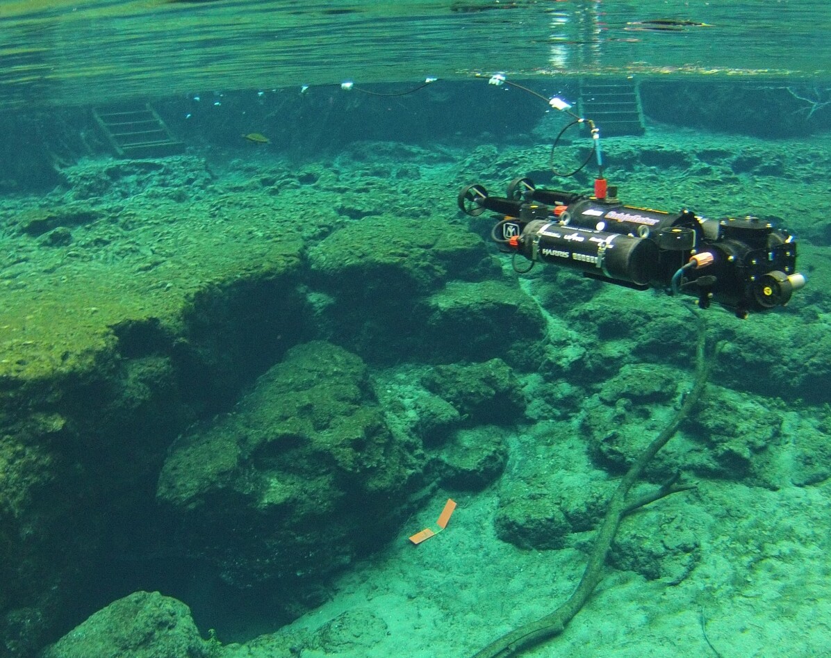
Figure 1: SubjuGator 7 AUV operating at Ginnie Springs, FL.

, is a small two man portable AUV with a mass of 40.8 kg. The vehicle is over-actuated with eight bidirectional thrusters.

Designed to be modular, the vehicle has multiple specialized pressure vessels that house computational capabilities, sensors, batteries, and mission specific payloads. The central pressure vessel houses the vehicle’s motor controllers, network infrastructure, and core computing capability. The core computing capability services the vehicles environmental sensors (e.g. visible light cameras, scanning sonar, etc.), the vehicles high-level mission planning, and low-level command and control software. A standard small form factor computer makes up the computing capability and utilizes a 2.13 GHz server grade quad-core processor. Located near the front of the vehicle, the navigation vessel houses the vehicle’s basic navigation sensors. The suite of navigation sensors include an inertial measurement unit, a Doppler velocity log (DVL), a depth sensor, and a digital compass. The navigation vessel also includes an embedded 720 MHz processor for preprocessing and packaging navigation data. Along the sides of the central pressure vessel, two vessels house 44 Ah of batteries used for propulsion and electronics.

The vehicle’s software runs within the Robot Operating System framework in the central pressure vessel. For the experiment, three main software nodes were used: navigation, control, and thruster mapping nodes. The navigation node receives packaged navigation data from the navigation pressure vessel where an extended Kalman filter estimates the vehicle’s full state at 50Hz. The controller node contains the developed controller and system identifier. The desired force and moment produced by the controller are mapped to the eight thrusters using a least-squares minimization algorithm in the thruster mapping node.

VII-B Controller Implementation

The implementation of the developed method involves: system identification, value function iteration, and control iteration. Implementing the system identifier requires (4), (6), and the data set described in Assumption 2. The data set in Assumption 2 was collected in a swimming pool. The vehicle was commanded to track an exciting trajectory with a robust integral of the sign of the error (RISE) controller [5] while the state-action pairs were recorded. The recorded data was trimmed to a subset of 40 sampled points that were selected to maximize the minimum singular value of $\left[\begin{array}[]{cccc}Y_{1}&Y_{2}&\ldots&Y_{j}\end{array}\right]$ as in Algorithm 1 of [14].

Evaluating the extrapolated Bellman error in (26) with each control iteration is computational expensive. Due to the limited computational resources available on-board the AUV, the value function weights were updated at a slower rate (i.e., 5Hz) than the main control loop (implemented at 50 Hz). The developed controller was used to control the surge, sway, and yaw states of the AUV, and a nominal controller was used to regulate the remaining states.

The vehicle uses water profiling data from the DVL to measure the relative water velocity near the vehicle in addition to bottom tracking data for the state estimator. By using the state estimator, water profiling data, and recorded data, the equations used to implement the proposed controller, i.e., (4), (6), (24), (26), and (28)-(31), only contain known or measurable quantities.

VII-C Results

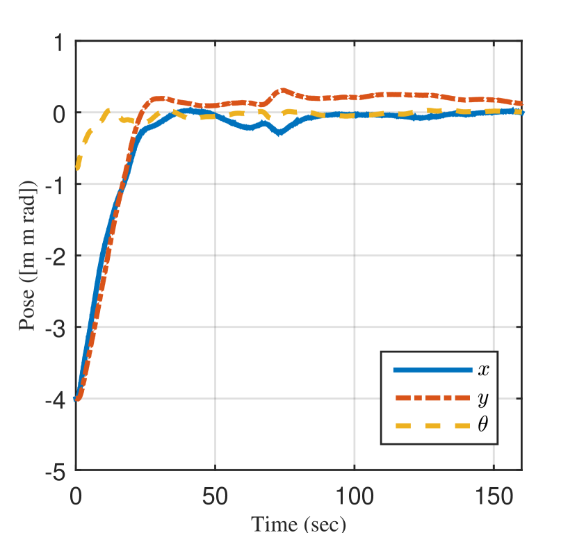
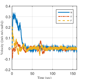
Figure 2: Inertial position error $\eta$ (top) and body-fixed velocity error $\nu$ (bottom) of the AUV.

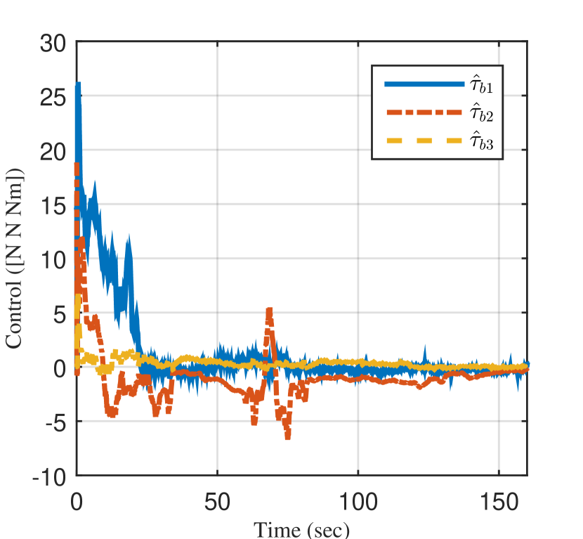
Figure 3: Body-fixed total control effort $\hat{\tau}_{b}$ commanded about the center of mass of the vehicle.

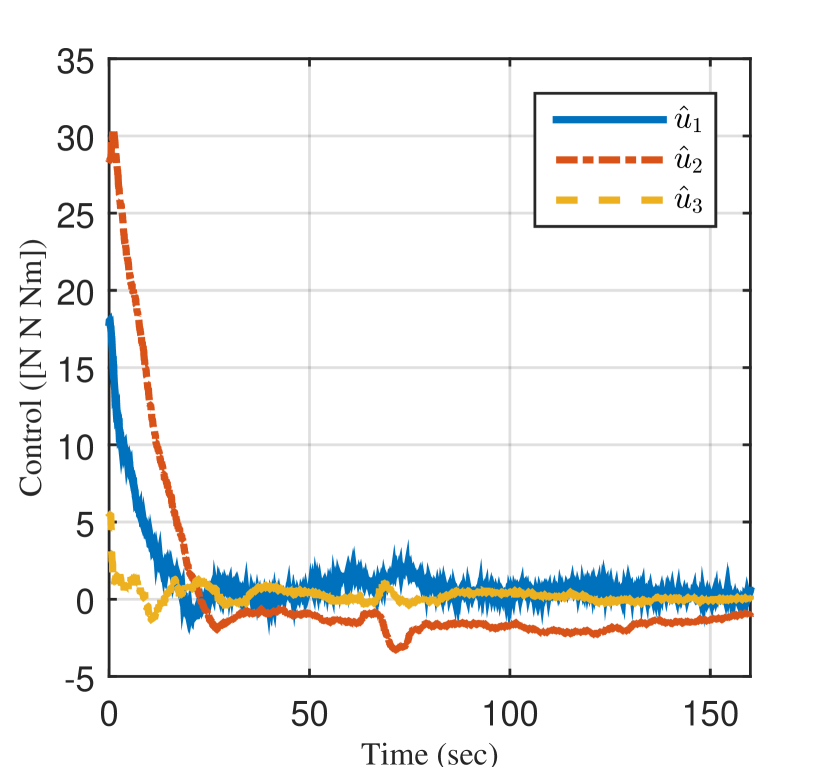
Figure 4: Body-fixed optimal control effort $\hat{u}$ commanded about the center of mass of the vehicle.

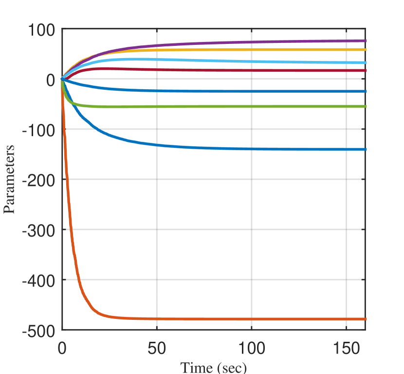
Figure 5: Identified system parameters determined for the vehicle online. The parameter definitions may be found in Example 6.2 and Equation 6.100 of [15].

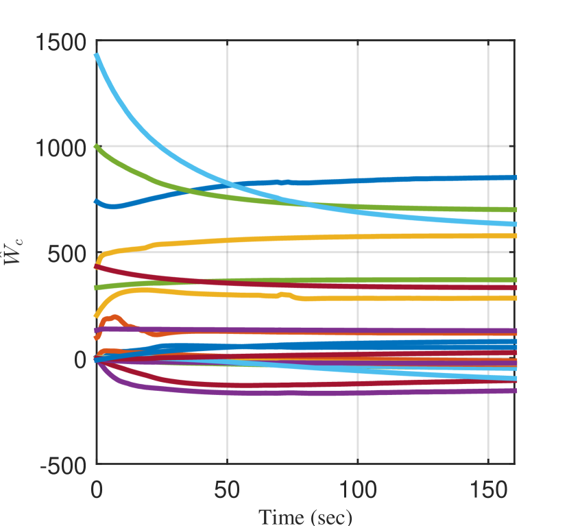
Figure 6: Critic $\hat{W}_{c}$ (top) and actor $\hat{W}_{a}$ (bottom) neural network weight estimates online convergence.

The vehicle was commanded to hold a station near the vent of Ginnie Spring. An initial condition of $\zeta\left(t_{0}\right)=\left[\begin{array}[]{cccccc}4\,\mathrm{m}&4\,\mathrm{m}&\frac{\pi}{4}\,\mathrm{rad}&0\,\mathrm{m/s}&0\,\mathrm{m/s}&0\,\mathrm{rad/s}\end{array}\right]^{T}$ was given to demonstrate the method’s ability to regulate the state. The optimal control weighting matrices were selected to be $Q=\mathrm{diag}\left(\left[20,50,20,10,10,10\right]\right)$ and $R=I_{3\times 3}$. The system identifier adaptation gains were selected to be $k_{\zeta}=25\times I_{6\times 6}$, $k_{\theta}=12.5$, and $\Gamma_{\theta}=\mbox{diag}\left(\left[187.5,937.5,37.5,37.5,37.5,37.5,37.5,37.5\right]\right)$. The parameter estimate was initialized with $\hat{\theta}\left(t_{0}\right)=0_{8\times 1}$. The neural network weights were initialized to match the ideal values for the linearized optimal control problem, which is obtained by solving the algebraic Riccati equation with the dynamics linearized about the station. The policy adaptation gains were chosen to be $k_{c1}=0.25$, $k_{c2}=0.5$, $k_{a}=1$, $k_{p}=0.25$, and $\beta=0.025$. The adaptation matrix was initialized to $\Gamma_{0}=400\times I_{21\times 21}$. The Bellman error was extrapolated to sampled states that were uniformly selected throughout the state space in the vehicle’s operating domain.

Figure 2 illustrates the ability of the generated policy to regulate the state in the presence of the spring’s current. Figure 3 illustrates the total control effort applied to the body of the vehicle, which includes the estimate of the current compensation term and approximate optimal control. Figure 4 illustrates the output of the approximate optimal policy for the residual system. Figure 5 illustrates the convergence of the parameters of the system identifier and Figure 6 illustrates convergence of the neural network weights representing the value function.

The anomaly seen at ~70 seconds in the total control effort (Figure 3) is attributed to a series of incorrect current velocity measurements. The corruption of the current velocity measurements is possibly due in part to the extremely low turbidity in the spring and/or relatively shallow operating depth. Despite presence of unreliable current velocity measurements the vehicle was able to regulate the vehicle to its station. The results demonstrate the developed method’s ability to concurrently identify the unknown hydrodynamic parameters and generate an approximate optimal policy using the identified model. The vehicle follows the generated policy to achieve its station keeping objective using industry standard navigation and environmental sensors (i.e., IMU, DVL).

VIII Conclusion

The online approximation of an optimal control strategy is developed to enable station keeping by an AUV. The solution to the HJB equation is approximated using adaptive dynamic programming. The hydrodynamic effects are identified online with a concurrent learning based system identifier. Leveraging the identified model, the developed strategy simulates exploration of the state space to learn the optimal policy without the need of a persistently exciting trajectory. A Lyapunov based stability analysis concludes UUB convergence of the states and UUB convergence of the approximated policies to the optimal polices. Experiments in a central Florida second-magnitude spring demonstrates the ability of the controller to generate and execute an approximate optimal policy in the presence of a time-varying irrational current.

IX Acknowledgment

The authors would like to thank Ginnie Springs Outdoors, LLC, who provided access to Ginnie Springs for the validation of the developed controller.

Appendix A Extension to constant earth-fixed current

In the case where the earth-fixed current is constant, the effects of the current may be included in the development of the optimal control problem. The body-relative current velocity $\nu_{c}\left(\zeta\right)$ is state dependent and may be determined from

$$\dot{\eta}_{c}=\left[\begin{array}[]{cc}\cos\left(\psi\right)&-\sin\left(\psi\right)\\ \sin\left(\psi\right)&\cos\left(\psi\right)\end{array}\right]\nu_{c},$$

where $\dot{\eta}_{c}\in\mathbb{R}^{n}$ is the known constant current velocity in the inertial frame. The functions $Y_{res}\theta$ and $f_{0_{res}}$ in (11) can then be redefined as

$$Y_{res}\theta\triangleq\left[\begin{array}[]{c}0\\ -M^{-1}C_{A}\left(-\nu_{c}\right)\nu_{c}-M^{-1}D\left(-\nu_{c}\right)\nu_{c}\ldots\\ -M^{-1}C_{A}\left(\nu_{r}\right)\nu_{r}-M^{-1}D\left(\nu_{r}\right)\nu_{r}\end{array}\right],$$

$$f_{0_{res}}\triangleq\left[\begin{array}[]{c}J_{E}\nu\\ -M^{-1}C_{RB}\left(\nu\right)\nu-M^{-1}G\left(\eta\right)\end{array}\right],$$

respectively. The control vector $u$ is

$$u=\tau_{b}-\tau_{c}$$

where $\tau_{c}\left(\zeta\right)\in\mathbb{R}^{n}$ is the control effort required to keep the vehicle on station given the current and is redefined as

$$\tau_{c}\triangleq-M_{A}\dot{\nu}_{c}-C_{A}\left(-\nu_{c}\right)\nu_{c}-D\left(-\nu_{c}\right)\nu_{c}.$$

References

• [1] A. J. Sørensen, “A survey of dynamic positioning control systems,” Annual Reviews in Control, vol. 35, pp. 123–136, 2011.
• [2] T. Fossen and A. Grovlen, “Nonlinear output feedback control of dynamically positioned ships using vectorial observer backstepping,” vol. 6, pp. 121–128, 1998.
• [3] E. Sebastian and M. A. Sotelo, “Adaptive fuzzy sliding mode controller for the kinematic variables of an underwater vehicle,” J. Intell. Robot. Syst., vol. 49, no. 2, pp. 189–215, 2007.
• [4] E. Tannuri, A. Agostinho, H. Morishita, and L. Moratelli Jr, “Dynamic positioning systems: An experimental analysis of sliding mode control,” Control Engineering Practice, vol. 18, pp. 1121–1132, 2010.
• [5] N. Fischer, D. Hughes, P. Walters, E. Schwartz, and W. E. Dixon, “Nonlinear RISE-based control of an autonomous underwater vehicle,” IEEE Trans. Robot., vol. 30, no. 4, pp. 845–852, Aug. 2014.
• [6] R. W. Beard and T. W. Mclain, “Successive galerkin approximation algorithms for nonlinear optimal and robust control,” Int. J. Control, vol. 71, no. 5, pp. 717–743, 1998.
• [7] S. Bhasin, R. Kamalapurkar, M. Johnson, K. G. Vamvoudakis, F. L. Lewis, and W. E. Dixon, “A novel actor-critic-identifier architecture for approximate optimal control of uncertain nonlinear systems,” Automatica, vol. 49, no. 1, pp. 89–92, Jan. 2013.
• [8] D. Vrabie and F. L. Lewis, “Neural network approach to continuous-time direct adaptive optimal control for partially unknown nonlinear systems,” Neural Netw., vol. 22, no. 3, pp. 237–246, 2009.
• [9] K. G. Vamvoudakis and F. L. Lewis, “Online actor-critic algorithm to solve the continuous-time infinite horizon optimal control problem,” Automatica, vol. 46, no. 5, pp. 878–888, 2010.
• [10] H. Modares, F. L. Lewis, and M.-B. Naghibi-Sistani, “Adaptive optimal control of unknown constrained-input systems using policy iteration and neural networks,” IEEE Trans. Neural Netw. Learn. Syst., vol. 24, no. 10, pp. 1513–1525, 2013.
• [11] ——, “Integral reinforcement learning and experience replay for adaptive optimal control of partially-unknown constrained-input continuous-time systems,” Automatica, vol. 50, no. 1, pp. 193–202, 2014.
• [12] M. Johnson, S. Bhasin, and W. E. Dixon, “Nonlinear two-player zero-sum game approximate solution using a policy iteration algorithm,” in Proc. IEEE Conf. Decis. Control, 2011, pp. 142–147.
• [13] K. G. Vamvoudakis and F. L. Lewis, “Online neural network solution of nonlinear two-player zero-sum games using synchronous policy iteration,” in Proc. IEEE Conf. Decis. Control, 2010.
• [14] G. Chowdhary, T. Yucelen, M. Mühlegg, and E. N. Johnson, “Concurrent learning adaptive control of linear systems with exponentially convergent bounds,” Int. J. Adapt. Control Signal Process., vol. 27, no. 4, pp. 280–301, 2013.
• [15] T. I. Fossen, Handbook of Marine Craft Hydrodynamics and Motion Control.   Wiley, 2011.
• [16] S. Sastry and A. Isidori, “Adaptive control of linearizable systems,” IEEE Trans. Autom. Control, vol. 34, no. 11, pp. 1123–1131, Nov. 1989.
• [17] P. Ioannou and J. Sun, Robust Adaptive Control.   Prentice Hall, 1996.
• [18] G. V. Chowdhary and E. N. Johnson, “Theory and flight-test validation of a concurrent-learning adaptive controller,” J. Guid. Control Dynam., vol. 34, no. 2, pp. 592–607, Mar. 2011.
• [19] R. Kamalapurkar, “Model-based reinforcement learning for online approximate optimal control,” Ph.D. dissertation, University of Florida, 2014.
• [20] A. Gelb, Applied optimal estimation.   The MIT press, 1974.
• [21] D. Kirk, Optimal Control Theory: An Introduction.   Mineola, NY: Dover, 2004.
• [22] R. Kamalapurkar, J. Klotz, and W. E. Dixon, “Concurrent learning-based online approximate feedback Nash equilibrium solution of N-player nonzero-sum differential games,” IEEE/CAA J. Autom. Sin., vol. 1, no. 3, pp. 239–247, Jul. 2014.
• [23] W. E. Dixon, A. Behal, D. M. Dawson, and S. Nagarkatti, Nonlinear Control of Engineering Systems: A Lyapunov-Based Approach.   Birkhauser: Boston, 2003.
• [24] H. K. Khalil, Nonlinear Systems, 3rd ed.   Upper Saddle River, NJ: Prentice Hall, 2002.
• [25] W. Schmidt, “Springs of Florida,” Florida Geological Survey, Bulletin 66, 2004.