ILAPF: Incremental Learning Assisted Particle Filtering

Abstract

This paper is concerned with dynamic system state estimation based on a series of noisy measurement with the presence of outliers. An incremental learning assisted particle filtering (ILAPF) method is presented, which can learn the value range of outliers incrementally during the process of particle filtering. The learned range of outliers is then used to improve subsequent filtering of the future state. Convergence of the outlier range estimation procedure is indicated by extensive empirical simulations using a set of differing outlier distribution models. The validity of the ILAPF algorithm is evaluated by illustrative simulations, and the result shows that ILAPF is more accurate and faster than a recently published state-of-the-art robust particle filter. It also shows that the incremental learning property of the ILAPF algorithm provides an efficient way to implement transfer learning among related state filtering tasks.

Index Terms—  incremental learning, outlier, particle filtering, robust state filtering, transfer learning

1 Introduction

State filtering plays a key role in the field of signal processing. This paper is concerned with nonlinear state filtering, for which the particle filter (PF) has been widely accepted as a well-established methodology for use [1, 2, 3, 4, 5, 6]. For conventional PF methods, a major degradation in performance will happen when a significant mismatch between the leveraged model and the real mechanism that governs the system’s evolution exists. A popular strategy to handle such issue of model mismatch is to employ a set of candidate models, instead of a single model, to take account of model uncertainty. To this end, a number of multiple-model strategies (MMS) based PF algorithms have been proposed in the literature [7, 8, 9, 10, 11].

In this paper, we consider the problem of nonlinear state filtering in presence of outliers. Instead of resorting to commonly used MMS that usually specify a set of candidate models beforehand to take account of model uncertainty, we select to learn an approximation of the outlier distribution in a sequential way. Specifically, we approximate the outlier distribution by a simple uniform distribution and then use an outlier range estimation (ORE) procedure to estimate the lower and upper bounds of that distribution. Convergence of the ORE procedure is indicated by extensive simulations as shown in Subsection 3.1. We incorporate the developed ORE operations into each iteration of PF, referring the resulting algorithm as Incremental Learning Assisted PF (ILAPF). This algorithm is shown to be robust against outliers, more accurate and faster than a robust PF method published in ICASSP 2017 [7], and can provide an efficient way to implement transfer learning among related state filtering tasks.

2 Model

In this Section, we present a succinct description of the model we use, based on which the ILAPF algorithm is developed. Following [7], we consider a state space model as follows

$$x_{k} = f(x_{k-1})+u_{k}$$ (1)

$$y_{k} = h(x_{k})+n_{k},$$ (2)

where $k$ denotes the time index, $x\in\mathbb{R}^{d_{x}}$ denotes the state of the dynamic system to be estimated, $y\in\mathbb{R}^{d_{y}}$ the measurement of $x_{k}$, $f$ the state transition function, $h$ the measurement function, $u$ the independent identically distributed (i.i.d.) process noise and $n$ the i.i.d. measurement noise. In a classical problem setting, the probability density functions (pdfs) of $u_{k}$ and $n_{k}$ are assumed a priori known, which determine the state transition prior density $p(x_{k}|x_{k-1})$ and the likelihood function $p(y_{k}|x_{k})$, respectively. Then using Bayesian theorem, we can formulate the state filtering problem as the computation of the a posteriori pdf of $x_{k}$ given $y_{1:k}\triangleq\{y_{1},\ldots,y_{k}\}$, denoted as $p(x_{k}|y_{1:k})$ (or in short $p_{k|k}$). Recursive solutions exist since $p_{k|k}$ can be computed from $p_{k-1|k-1}$ recursively as follows

$$p_{k|k}=\frac{p(y_{k}|x_{k})\int p(x_{k}|x_{k-1})p_{k-1|k-1}dx_{k-1}}{p(y_{k}|y_{1:k-1})}.$$ (3)

Here we bring a variable $o\in\{0,1\}$ to take account of the uncertainty in the measurement model. Specifically, let $o_{k}=1(0)$ denote the event that $y_{k}$ is (is not) an outlier. If $o_{k}=0$ we assume that the measurement noise $n_{k}$ is Gaussian distributed by default, namely $n_{k}\sim\mathcal{N}(0,R)$, where $R$ is a priori known. If $o_{k}=1$ we assume that $n_{k}$ is generated from an unknown uniform distribution $\mathcal{U}(lb,ub)$, where $lb$ and $ub$ denote the lower and upper bounds of $\mathcal{U}$, respectively. The likelihood function can now be represented as follows

$$p(y_{k}|x_{k})=\left\{\begin{array}[]{ll}p(y_{k}|x_{k},o_{k}=1),\quad\mbox{if}\quad o_{k}=1\\ p(y_{k}|x_{k},o_{k}=0),\quad\mbox{if}\quad o_{k}=0\end{array}\right.$$ (4)

where

$$p(y_{k}|x_{k},o_{k}=1) = \left\{\begin{array}[]{ll}1/V_{lb,ub},\quad\mbox{if}\quad e_{k}\in[lb,ub]\\ 0,\quad\mbox{otherwise}\end{array}\right.$$ (7)

$$p(y_{k}|x_{k},o_{k}=0) = \mathcal{N}\left(e_{k}|0,R\right),$$ (8)

where $e_{k}=y_{k}-h(x_{k})$ and $V_{lb,ub}$ denotes the volume of the space bounded by $lb$ and $ub$. An ORE procedure is developed to estimate $lb$ and $ub$ incrementally, see details in Subsection 3.1.

3 The proposed ILAPF Algorithm

Here we present the ILAPF algorithm used to address the Bayesian state filtering problem defined by Eqns.(1)-(6). Suppose that, at time step $k-1$ ($k>1$), we have a discrete approximation of $p(x_{1:k-1}|y_{1:k-1})$ given by a set of weighted samples $\{x_{1:k-1}^{i},\omega_{k-1}^{i}\}_{i=1}^{N}$, $\sum_{i=1}^{N}\omega_{k-1}^{i}=1$. At time $k$, the $i$th sample is first extended by a particle $\hat{x}_{k}^{i}=f(x_{k-1}^{i})$. Then, according to importance sampling theory [12, 1, 13], it is weighted by

$$\omega_{m,k}^{i}=\omega_{k-1}^{i}p(y_{k}|\hat{x}_{k}^{i},o_{k}=m),$$ (9)

under the hypothesis $o_{k}=m$, $m=0,1$. Then the likelihood of the event $o_{k}=m$ is given by

$$L(o_{k}=m)=\sum_{i=1}^{N}\omega_{m,k}^{i}.$$ (10)

Assume that the prior probability $p(o_{k}=0)=p(o_{k}=1)=0.5$. From Bayesian theorem the posterior probability of $o_{k}=m$ is given by

$$\pi(o_{k}=m)=\frac{L(o_{k}=m)}{L(o_{k}=0)+L(o_{k}=1)},m=0,1.$$ (11)

Then the importance weights of the particles can be calculated as follows

$$\omega_{k}^{i}\varpropto\sum_{m=\{0,1\}}\pi(o_{k}=m)\tilde{\omega}_{m,k}^{i},i=1,\ldots,N,$$ (12)

where $\tilde{\omega}_{m,k}^{i}=\omega_{m,k}^{i}/\sum_{j=1}^{N}\omega_{m,k}^{j}$. To get around of particle degeneracy, we use a resampling step to discard the particles with low weights and duplicate those with high weights. For details on resampling techniques used by PF methods, readers are referred to [14, 15, 16].

The above operations constitute the major building block of the ILAPF algorithm, while a crucial issue is neglected, that is how to compute $p(y_{k}|\hat{x}_{k}^{i},o_{k}=1)$ in Eqn. (9) with an unknown outlier distribution. We present the ORE procedure in Subsection 3.1 to address the above issue, and then summarize the operations of ILAPF in Subsection 3.2.

3.1 The outlier range estimation (ORE) procedure

Assume that the whole population of the outliers has a definite value range specified by a lower and upper bounds $lb$ and $ub$. We can estimate $lb$ and $ub$ accurately provided that we have enough outlier data points at hand. But in practical tasks, usually, only a sparse set of outliers can be collected in a sequential way. The question under consideration here is: how to estimate $lb$ and $ub$ accurately using a limited number of outliers that have been found? To fit the sequential structure of the state filtering problem, we also expect that the estimation procedure can be performed in a sequential way.

We develop an ORE method to address the above problem. This method only has one free parameter $I$, which can be interpreted as a measure of uncertainty. In ORE method, we consider outliers sequentially, making an incremental update to the estimation of $lb$ and $ub$, once a new outlier arrives. Assume that the current estimations of $lb$ and $ub$ are $\hat{lb}$ and $\hat{ub}$, respectively, and the number of outliers that have been found is $n$. When the $(n+1)$th outlier, denoted as $z_{n+1}$, arrives, the ORE procedure updates $\hat{lb}$ and $\hat{ub}$ as follows

$$\hat{lb} = \min\{\hat{lb},z_{n+1}\}-I/(n+1),$$ (13)

$$\hat{ub} = \max\{\hat{ub},z_{n+1}\}+I/(n+1).$$ (14)

We tested the validity of the ORE method via simulations. We used 4 differing outlier distributions to simulate the outliers, including a Uniform $\mathcal{U}(40,50)$, a Gaussian $\mathcal{N}(45,1)$, a Student’s t and a two-component Gaussian mixture distribution $0.5\mathcal{N}(45,1)+0.5\mathcal{N}(47,1)$. The Student’s t distribution has a degree of freedom 3, mean 45 and standard error 1. The ORE procedure is initialized with $\hat{lb}=20$ and $\hat{ub}=70$, which represent an initial guess of the bounds. We considered 4 values of $I$, namely 10, 40, 70 and 100. For each $I$ value and each outlier distribution, we ran the ORE method to process the data items that arrive one by one. We recorded the estimated bounds at each time step when an outlier arrives, and the result is shown in Fig.1. We see that, for every distribution case, the estimated bounds converge to the desired ones and the convergence rate depends on the value of $I$. Specifically, Fig.1 shows that an $I$ value between 10 and 40 will be best for choice. So for the simulated experiments presented in Section 4, the value of $I$ is set at 20. Note that we take mean$\pm 3\times$standard error as the desired bounds for the Gaussian and Student’s t cases, and $m_{1}-3\sigma$ and $m_{2}+3\sigma$ for the Gaussian mixture case, where $m_{1}$ and $m_{2}$ denote the smaller and bigger mean value, $\sigma$ standard error of those 2 mixing Gaussian components.

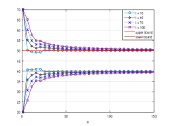
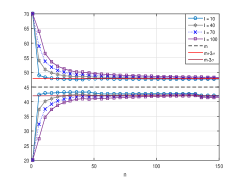
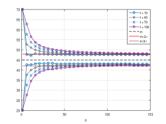
Fig. 1: The simulation result of using the ORE procedure to sequentially estimate the range of the outliers. 4 distributions to generate the outliers are considered, including the Uniform, Gaussian, Student’s t and a two-component Gaussian mixture distribution, corresponding to the top left, top right, bottom left and bottom right panel, respectively. The X-coordinate represents the number of outliers that have been detected and the Y-coordinate the value of the outliers. $m$ and $\sigma$ denote the mean and the standard error of a related distribution, respectively. In the bottom right panel, $m_{1}$ and $m_{2}$ represent the smaller and bigger mean of the two Gaussian components that have the same standard error $\sigma$.

3.2 A summarization of the operations in ILAPF

Starting from $\{x_{k-1}^{i},\omega_{k-1}^{i}\}_{i=1}^{N}$, $\hat{lb}$ and $\hat{ub}$ and the number of outliers that have been found $n$, we present operations in one iteration of the ILAPF algorithm corresponding to time step $k$ as follows.

• Sampling step. Sample $\hat{x}_{k}^{i}$ from the state transition prior by setting $\hat{x}_{k}^{i}=f(x_{k-1}^{i})$, $i=1,\ldots,N$;

• Weighting step. Set $\omega_{m,k}^{i}$ using Eqn.(9), $i=1,\ldots,N$. Compute $\pi(o_{k}=1)$ and $\pi(o_{k}=0)$ using Eqn. (11). Calculate importance weight $\omega_{k}^{i}$ using Eqn. (12), $i=1,\ldots,N$. Then normalize these weights to guarantee that $\sum_{i=1}^{N}\omega_{k}^{i}=1$;

• ORE step. If $\pi(o_{k}=1)>0.5$, declare $y_{k}$ to be an outlier, let $n=n+1$ and update $\hat{lb}$ and $\hat{ub}$ using Eqns. (11) and (12), respectively. Note that $\pi(o_{k}=1)$ is an output of the above weighting step.

• Resampling step. Sample $x_{k}^{i}\sim\sum_{j=1}^{N}\omega_{k}^{j}\delta_{\hat{x}_{k}^{j}}$, set $\omega_{k}^{i}=1/N$, $i=1,\ldots,N$. $\delta_{x}$ denotes the Dirac-delta function located at $x$.

4 Performance Evaluation

We evaluated the validity of ILAPF via illustrative simulations. A recently published heterogeneous mixture model based robust PF (HMM-RPF) [7] was included for performance comparison.

4.1 Simulation Setting

The simulation setting is similar as that in [7]. We design a modified version of the time-series experiment as presented in [17] by replacing some normal measurements with outliers. The time-series is generated as follows

$$x_{k+1}=1+\sin(0.04\pi\times(k+1))+0.5x_{k}+u_{k},1\leq k<60,$$ (15)

with the value of $x_{1}$ set at 1, and $u_{k}$ represented as a Gamma(3,2) random variable modeling the process noise. The measurement model is

$$y_{k}=\left\{\begin{array}[]{ll}0.2x_{k}^{2}+n_{k},\quad\quad\quad k\leq 30\\ 0.2x_{k}-2+n_{k},\quad\,k>30\end{array}\right.$$ (16)

The measurement noise $n_{k}$ is Gaussian distributed by default with mean 0 and variance 0.01. The outliers arrive at time steps $k=7,8,9,20,37,38,39,50$. Each outlier is simulated by replacing the default Gaussian distribution with a uniform distribution $\mathcal{U}(20,30)$ in generating the value of $n_{k}$ in Eqn.(16). The state filtering algorithms to be tested are set to be blind to both the arrival time and the generative distribution of the outliers.

4.2 Results

Based on the above simulation setting, we first simulated a time-series and then ran the ILAPF and HMM-RPF [7] to process the data, respectively. The ILAPF is initialized with $\hat{lb}=0$, $\hat{ub}=70$ and $I=20$. The value range [0, 70] represents a vague initial guess for the real value range [20, 30]. An $I$ value 20 is selected based on the simulation results as shown in Fig. 1. The HMM-RPF algorithm in use is the same as that presented in [7] with the forgetting factor $\alpha$ set at 0.9. For both ILAPF and HMM-RPF, a particle size $N=200$ is used. The state filtering and the posterior model/hypothesis inference results are shown in Figs.2 and 3, respectively.

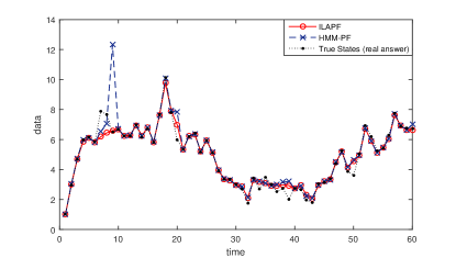
Fig. 2: Filtering result of ILAPF and HMM-RPF [7].

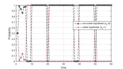
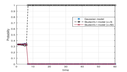
Fig. 3: The top panel shows the ILAPF yielded posterior probabilities of the outlier hypothesis (corresponding to $o_{k}=1$) and the non-outlier hypothesis (corresponding to $o_{k}=0$). The bottom panel shows the HMM-RPF [7] yielded posterior probabilities of the candidate models it employs and v denotes the degree of freedom of a Student’s t model. The real arrival time steps of the outliers are $7,8,9,20,37,38,39,50$.

Table 1: Execution time (in seconds), Mean and variance of the MSE calculated over 30 independent runs of each algorithm.

Algorithm	Time	MSE
		mean	var
ILAPF	3.998	0.365	0.007
HMM-RPF [7]	5.509	0.582	0.109

Table 2: Mean and variance of the MSE calculated over 30 independent runs of ILAPF for 4 consecutive tasks.

	Task 1	Task 2	Task 3	Task 4
Mean of MSE	0.365	0.360	0.333	0.272
Variance of MSE	0.007	0.005	0.004	0.003

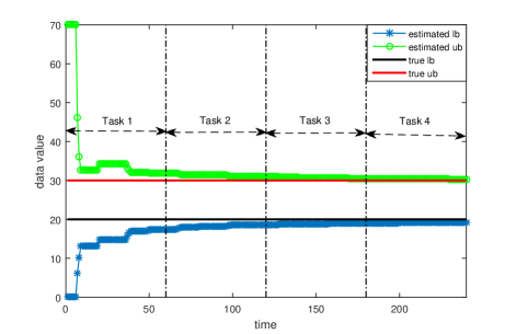
Fig. 4: The estimated lower and upper bounds of the outliers’ value range over 4 consecutive state filtering tasks

We then conducted a Monte Carlo test for the involved algorithms. We did the above experiment 30 times and then calculated the mean of execution time (in seconds), the means and variances of the mean-square-error (MSE) of the state estimates over these experiments for each algorithm. The result is summarized in Table 1.

Finally, we tested whether the incremental learning property of the ILAPF can provide benefits to implement a transfer learning among related state filtering tasks. We simulated 4 consecutive tasks of state filtering in presence of outliers. For each task, the experimental setting is totally the same as presented in Subsection 4.1. The ILAPF is run for each task one by one, and the learned value bounds of the outliers from one task are used to initialize ILAPF for the subsequent task. The estimated bound over these 4 tasks is shown in Fig.4 and a quantitative MSE result corresponding to 30 independent runs of the ILAPF for 4 consecutive tasks is presented in Table 2. We see that, with aid of ILAPF, the learned information on outliers from one task can be transferred to subsequent tasks, resulting in a continuous incremental performance gain, in terms of MSE, over tasks.

5 Conclusions

MMS is a powerful solution to address nonlinear state filtering problems in presence of model uncertainty. The common practice to implement MMS is to specify a set of candidate models beforehand. In this paper, we proposed a novel way to implement MMS in the context of nonlinear state filtering in presence of outliers. Instead of specifying a set of candidate models beforehand, we select to learn a model to approximate the distribution of the outliers in a sequential way. The resulting algorithm, ILAPF, is shown to be more accurate and faster than its competitor algorithm HMM-RPF [7]. Through simulations, we also show that the ILAPF algorithm makes transfer learning among related state filtering tasks possible.

References

- [1] M. S. Arulampalam, S. Maskell, N. Gordon, and T. Clapp, “A tutorial on particle filters for online nonlinear/non-Gaussian Bayesian tracking,” IEEE Trans. on Signal Processing, vol. 50, no. 2, pp. 174–188, 2002.
- [2] J. Carpenter, P. Clifford, and P. Fearnhead, “Improved particle filter for nonlinear problems,” IEE Proceedings-Radar, Sonar and Navigation, vol. 146, no. 1, pp. 2–7, 1999.
- [3] N. J. Gordon, D. J. Salmond, and A. FM Smith, “Novel approach to nonlinear/non-gaussian bayesian state estimation,” IEE Proceedings F (Radar and Signal Processing), vol. 140, no. 2, pp. 107–113, 1993.
- [4] B Liu, C Ji, Y Zhang, C Hao, and K-K Wong, “Multi-target tracking in clutter with sequential Monte Carlo methods,” IET radar, sonar & navigation, vol. 4, no. 5, pp. 662–672, 2010.
- [5] B. Liu and C. Hao, “Sequential bearings-only-tracking initiation with particle filtering method,” The Scientific World Journal, vol. 2013, pp. 1–7, 2013.
- [6] B. Liu, X. Ma, and C. Hou, “A particle filter using SVD based sampling Kalman filter to obtain the proposal distribution,” in Proc. of IEEE Conf. on Cybernetics and Intelligent Systems. IEEE, 2008, pp. 581–584.
- [7] B. Liu, “Robust particle filter by dynamic averaging of multiple noise models,” in Proc. of the 42nd IEEE Int’l Conf. on Acoustics, Speech, and Signal Processing (ICASSP). IEEE, 2017, pp. 4034–4038.
- [8] Y. Dai and B. Liu, “Robust video object tracking via Bayesian model averaging-based feature fusion,” Optical Engineering, vol. 55, no. 8, pp. 083102(1)–083102(11), 2016.
- [9] B. Liu, “Instantaneous frequency tracking under model uncertainty via dynamic model averaging and particle filtering,” IEEE Trans. on Wireless Communications, vol. 10, no. 6, pp. 1810–1819, 2011.
- [10] C. C. Drovandi, J. Mcgree, and A. N. Pettitt, “A Sequential Monte Carlo algorithm to incorporate model uncertainty in Bayesian sequential design,” Journal of Computational and Graphical Statistics, vol. 23, no. 1, pp. 3–24, 2014.
- [11] U. Iñigo, F. B. Mónica, and M. D. Petar, “Sequential Monte Carlo methods under model uncertainty,” in Proc. of IEEE Statistical Signal Processing Workshop (SSP). IEEE, 2016, pp. 1–5.
- [12] A. Doucet, S. Godsill, and C. Andrieu, “On Sequential Monte Carlo sampling methods for Bayesian filtering,” Statistics and Computing, vol. 10, no. 3, pp. 197–208, 2000.
- [13] A. Smith, A. Doucet, N. de Freitas, and N. Gordon, Sequential Monte Carlo methods in practice, Springer Science & Business Media, 2013.
- [14] Randal Douc and Olivier Cappé, “Comparison of resampling schemes for particle filtering,” in Proc. of the 4th Int’l Symp. on Image and Signal Processing and Analysis (ISPA). IEEE, 2005, pp. 64–69.
- [15] T. Li, M. Bolic, and P. M. Djuric, “Resampling methods for particle filtering: classification, implementation, and strategies,” IEEE Signal Processing Magazine, vol. 32, no. 3, pp. 70–86, 2015.
- [16] J. D. Hol, T. B. Schon, and Gustafsson F., “On resampling algorithms for particle filters,” in Proc. of the IEEE Nonlinear Statistical Signal Processing Workshop (NSSPW). IEEE, 2006, pp. 79–82.
- [17] R. Van Der Merwe, A. Doucet, N. De Freitas, and E. Wan, “The unscented particle filter,” in NIPS, 2000, pp. 584–590.