Attention-Based Models for Text-Dependent Speaker Verification

Abstract

Attention-based models have recently shown great performance on a range of tasks, such as speech recognition, machine translation, and image captioning due to their ability to summarize relevant information that expands through the entire length of an input sequence. In this paper, we analyze the usage of attention mechanisms to the problem of sequence summarization in our end-to-end text-dependent speaker recognition system. We explore different topologies and their variants of the attention layer, and compare different pooling methods on the attention weights. Ultimately, we show that attention-based models can improves the Equal Error Rate (EER) of our speaker verification system by relatively 14% compared to our non-attention LSTM baseline model.

Index Terms—  Attention-based model, sequence summarization, speaker recognition, pooling, LSTM

1 Introduction

Speaker verification (SV) is the process of verifying, based on a set of reference enrollment utterances, whether an verification utterance belongs to a known speaker. One subtask of SV is global password text-dependent speaker verification (TD-SV), which refers to the set of problems for which the transcripts of reference enrollment and verification utterances are constrained to a specific phrase. In this study, we focus on “OK Google” and “Hey Google” global passwords, as they relate to the Voice Match feature of Google Home [1, 2].

I-vector [3] based systems in combination with verification back-ends such as Probabilistic Linear Discriminant Analysis (PLDA) [4] have been the dominating paradigm of SV in previous years. More recently, with the rising of deep learning [5] in various machine learning applications, more efforts have been focusing on using neural networks for speaker verification. Currently, the most promising approaches are end-to-end integrated architectures that simulate the enrollment-verification two-stage process during training.

For example, in [6] the authors propose architectures that resemble the components of an i-vector + PLDA system. Such architecture allowed to bootstrap the network parameters from pretrained i-vector and PLDA models for a better performance. However, such initialization stage also constrained the type of network architectures that could be used — only Deep Neural Networks (DNN) can be initialized from classical i-vector and PLDA models. In [7], we have shown that Long Short-Term Memory (LSTM) networks [8] can achieve better performance than DNNs for integrated end-to-end architectures in TD-SV scenarios.

However, one challenge in our architecture introduced in [7] is that, silence and background noise are not being well captured. Though our speaker verification runs on a short 800ms window that is segmented by the keyword detector [9, 10], the phonemes are usually surrounded by frames of silence and background noise. Ideally, the speaker embedding should be built only using the frames corresponding to phonemes. Thus, we propose to use an attention layer [11, 12, 13] as a soft mechanism to emphasize the most relevant elements of the input sequence.

This paper is organized as follows. In Sec. 2, we first briefly review our LSTM-based d-vector baseline approach trained with the end-to-end architecture [7]. In Sec. 3, we introduce how we add the attention mechanism to our baseline architecture, covering different scoring functions, layer variants, and weights pooling methods. In Sec. 4 we setup experiments to compare attention-based models against our baseline model, and present the EER results on our testing set. Conclusions are made in Sec. 5.

2 Baseline Architecture

Our end-to-end training architecture [7] is described in Fig. 1. For each training step, a tuple of one evaluation utterance $\mathbf{x}_{j\sim}$ and $N$ enrollment utterances $\mathbf{x}_{kn}$ (for $n=1,\cdots,N$) is fed into our LSTM network: $\{\mathbf{x}_{j\sim},(\mathbf{x}_{k1},\cdots,\mathbf{x}_{kN})\}$, where $\mathbf{x}$ represents the features (log-mel-filterbank energies) from a fixed-length segment, $j$ and $k$ represent the speakers of the utterances, and $j$ may or may not equal $k$. The tuple includes a single utterance from speaker $j$, and $N$ different utterance from speaker $k$. We call a tuple positive if ${\mathbf{x}}_{j\sim}$ and the $N$ enrollment utterances are from the same speaker, i.e., $j=k$, and negative otherwise. We generate positive and negative tuples alternatively.

For each utterance, let the output of the LSTM’s last layer at frame $t$ be a fixed dimensional vector $\mathbf{h}_{t}$, where $1\leq t\leq T$. We take the last frame output as the d-vector $\boldsymbol{\omega}=\mathbf{h}_{T}$ (Fig. 2a), and build a new tuple: $\{\boldsymbol{\omega}_{j\sim},(\boldsymbol{\omega}_{k1},\cdots,\boldsymbol{\omega}_{kN})\}$. The centroid of tuple $(\boldsymbol{\omega}_{k1},\cdots,\boldsymbol{\omega}_{kN})$ represents the voiceprint built from $N$ utterances, and is defined as follows:

$$\mathbf{c}_{k}=\mathrm{E}_{n}[\boldsymbol{\omega}_{kn}]=\frac{1}{N}\sum_{n=1}^{N}\dfrac{\boldsymbol{\omega}_{kn}}{\mathbin{\|}\boldsymbol{\omega}_{kn}\mathbin{\|}_{2}}.$$ (1)

The similarity is defined using the cosine similarity function:

$$s=w\cdot\cos(\boldsymbol{\omega}_{j\sim},\mathbf{c}_{k})+b,$$ (2)

with learnable $w$ and $b$. The tuple-based end-to-end loss is finally defined as:

$$L_{\mathrm{T}}(\boldsymbol{\omega}_{j\sim},\mathbf{c}_{k})=\delta(j,k)\sigma(s)+\Big{(}1-\delta(j,k)\Big{)}\Big{(}1-\sigma(s)\Big{)}.$$ (3)

Here $\sigma(x)=1/(1+e^{-x})$ is the standard sigmoid function and $\delta(j,k)$ equals $1$ if $j=k$, otherwise equals to $0$. The end-to-end loss function encourages a larger value of $s$ when $k=j$, and a smaller value of $s$ when $k\neq j$. Consider the update for both positive and negative tuples — this loss function is very similar to the triplet loss in FaceNet [14].

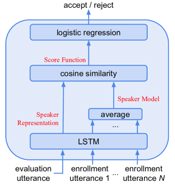
Fig. 1: Our baseline end-to-end training architecture as introduced in [7].

3 Attention-based model

3.1 Basic attention layer

In our baseline end-to-end training, we directly take the last frame output as d-vector $\boldsymbol{\omega}=\mathbf{h}_{T}$. Alternatively, we could learn a scalar score $e_{t}\in\mathbb{R}$ for the LSTM output $\mathbf{h}_{t}$ at each frame $t$:

$$e_{t}=f(\mathbf{h}_{t}),\qquad t=1,\cdots,T.$$ (4)

Then we can compute the normalized weights $\alpha_{t}\in[0,1]$ using these scores:

$$\alpha_{t}=\dfrac{\exp(e_{t})}{\sum_{i=1}^{T}\exp(e_{i})},$$ (5)

such that $\sum_{t=1}^{T}\alpha_{t}=1$. And finally, as shown in Fig. 2b, we form the d-vector $\boldsymbol{\omega}$ as the weighted average of the LSTM outputs at all frames:

$$\boldsymbol{\omega}=\sum_{t=1}^{T}\alpha_{t}\mathbf{h}_{t}.$$ (6)

3.2 Scoring functions

By using different scoring functions $f(\cdot)$ in Eq. (4), we get different attention layers:

• Bias-only attention, where $b_{t}$ is a scalar. Note this attention does not depend on the LSTM output $\mathbf{h}_{t}$.

  $$e_{t}=f_{\mathrm{BO}}(\mathbf{h}_{t})=b_{t}.$$ (7)

• Linear attention, where $\mathbf{w}_{t}$ is an $m$-dimensional vector, and $b_{t}$ is a scalar.

  $$e_{t}=f_{\mathrm{L}}(\mathbf{h}_{t})=\mathbf{w}_{t}^{T}\mathbf{h}_{t}+b_{t}.$$ (8)

• Shared-parameter linear attention, where the $m$-dimensional vector $\mathbf{w}$ and scalar $b$ are the same for all frames.

  $$e_{t}=f_{\mathrm{SL}}(\mathbf{h}_{t})=\mathbf{w}^{T}\mathbf{h}_{t}+b.$$ (9)

• Non-linear attention, where $\mathbf{W}_{t}$ is an $m^{\prime}\times m$ matrix, $\mathbf{b}_{t}$ and $\mathbf{v}_{t}$ are $m^{\prime}$-dimensional vectors. The dimension $m^{\prime}$ can be tuned on a development dataset.

  $$e_{t}=f_{\mathrm{NL}}(\mathbf{h}_{t})=\mathbf{v}_{t}^{T}\tanh(\mathbf{W}_{t}\mathbf{h}_{t}+\mathbf{b}_{t}).$$ (10)

• Shared-parameter non-linear attention, where the same $\mathbf{W}$, $\mathbf{b}$ and $\mathbf{v}$ are used for all frames.

  $$e_{t}=f_{\mathrm{SNL}}(\mathbf{h}_{t})=\mathbf{v}^{T}\tanh(\mathbf{W}\mathbf{h}_{t}+\mathbf{b}).$$ (11)

In all the above scoring functions, all the parameters are trainable within the end-to-end architecture [7].

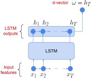
(a)

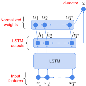
(b)

Fig. 2: (a) LSTM-based d-vector baseline [7]. (b) Basic attention layer.

3.3 Attention layer variants

Apart from the basic attention layer described in Sec. 3.1, here we introduce two variants: cross-layer attention, and divided-layer attention.

For cross-layer attention (Fig. 3a), the scores $e_{t}$ and weights $\alpha_{t}$ are not computed using the outputs of the last LSTM layer $\{\mathbf{h}_{t}\}_{1\leq t\leq T}$, but the outputs of an intermediate LSTM layer $\{\mathbf{h}^{\prime}_{t}\}_{1\leq t\leq T}$, e.g. the second-to-last layer:

$$e_{t}=f(\mathbf{h}^{\prime}_{t}).$$ (12)

However, the d-vector $\boldsymbol{\omega}$ is still the weighted average of the last layer output $\mathbf{h}_{t}$.

For divided-layer attention (Fig. 3b), we double the dimension of the last layer LSTM output $\mathbf{h}_{t}$, and equally divide its dimension into two parts: part-a $\mathbf{h}_{t}^{a}$, and part-b $\mathbf{h}_{t}^{b}$. We use part-a to build the d-vector, while using part-b to learn the scores:

$$e_{t}=f(\mathbf{h}_{t}^{b}),$$ (13)

$$\boldsymbol{\omega}=\sum_{t=1}^{T}\alpha_{t}\mathbf{h}_{t}^{a}.$$ (14)

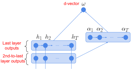
(a)

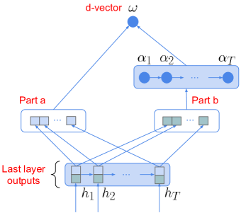
(b)

Fig. 3: Two variants of the attention layer: (a) cross-layer attention; (b) divided-layer attention.

3.4 Weights pooling

Another variation of the basic attention layer is that, instead of directly using the normalized weights $\alpha_{t}$ to average LSTM outputs, we can optionally perform maxpooling on the attention weights. This additional pooling mechanism can potentially make our network more robust to temporal variations of the input signals. We have experimented with two maxpooling methods (Fig. 4):

• Sliding window maxpooling: We run a sliding window on the weights, and for each window, only keep the largest value, and set other values to 0.

• Global top-$K$ maxpooling: Only keep the largest $K$ values in the weights, and set all other values to 0.

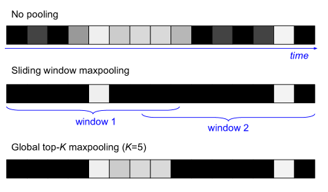
Fig. 4: Different pooling methods on attention weights. The $t$th pixel corresponds to the weight $\alpha_{t}$, and a brighter intensity means a larger value of the weight.

4 Experiments

4.1 Datasets and basic setup

To fairly compare different attention techniques, we use the same training and testing datasets for all our experiments.

Our training dataset is a collection of anonymized user voice queries, which is a mixture of “OK Google” and “Hey Google”. It has around 150M utterances from around 630K speakers. Our testing dataset is a manual collection consisting of 665 speakers. It’s divided into two enrollment sets and two verification sets for each of “OK Google” and “Hey Google”. Each enrollment and evaluation dataset contains respectively, an average of 4.5 and 10 evaluation utterances per speaker.

We report the speaker verification Equal Error Rate (EER) on the four combinations of enrollment set and verification set.

Our baseline model is a 3-layer LSTM, where each layer has dimension 128, with a projection layer [15] of dimension 64. On top of the LSTM is a linear layer of dimension 64. The acoustic parametrization consists of 40-dimensional log-mel-filterbank coefficients computed over a window of 25ms with 15ms of overlap. The same acoustic features are used for both keyword detection [10] and speaker verification.

The keyword spotting system isolates segments of length $T=80$ frames (800ms) that only contain the global password, and these segments form the tuples mentioned above. The two keywords are mixed together using the MultiReader technique introduced in [16].

4.2 Basic attention layer

First, we compare the baseline model with basic attention layer (Sec. 3.1) using different scoring function (Sec. 3.2). The results are shown in Table 1. As we can see, while bias-only and linear attention bring little improvement to the EER, non-linear attention improves the performance significantly, especially with shared parameters.

Table 1: Evaluation EER(%): Non-attention baseline model vs. basic attention layer using different scoring functions.

Test data	Non-attention	Basic attention
Enroll $\rightarrow$ Verify	baseline	$f_{\mathrm{BO}}$	$f_{\mathrm{L}}$	$f_{\mathrm{SL}}$	$f_{\mathrm{NL}}$	$f_{\mathrm{SNL}}$
OK Google $\rightarrow$ OK Google	0.88	0.85	0.81	0.8	0.79	0.78
OK Google $\rightarrow$ Hey Google	2.77	2.97	2.74	2.75	2.69	2.66
Hey Google $\rightarrow$ OK Google	2.19	2.3	2.28	2.23	2.14	2.08
Hey Google $\rightarrow$ Hey Google	1.05	1.04	1.03	1.03	1.00	1.01
Average	1.72	1.79	1.72	1.70	1.66	1.63

4.3 Variants

To compare the basic attention layer with the two variants (Sec. 3.3), we use the same scoring function that performs the best in the previous experiment: the shared-parameter non-linear scoring function $f_{\mathrm{SNL}}$. From the results in Table 2, we can see that divided-layer attention performs slightly better than basic attention and cross-layer attention, at the cost that the dimension of last LSTM layer is doubled.

Table 2: Evaluation EER(%): Basic attention layer vs. variants — all using $f_{\mathrm{SNL}}$ as scoring function.

Test data	Basic $f_{\mathrm{SNL}}$	Cross-layer	Divided-layer
OK $\rightarrow$ OK	0.78	0.81	0.75
OK $\rightarrow$ Hey	2.66	2.61	2.44
Hey $\rightarrow$ OK	2.08	2.03	2.07
Hey $\rightarrow$ Hey	1.01	0.97	0.99
Average	1.63	1.61	1.56

Table 3: Evaluation EER(%): Different pooling methods for attention weights — all using $f_{\mathrm{SNL}}$ and divided-layer.

Test data	No pooling	Sliding window	Top-$K$
OK $\rightarrow$ OK	0.75	0.72	0.72
OK $\rightarrow$ Hey	2.44	2.37	2.63
Hey $\rightarrow$ OK	2.07	1.88	1.99
Hey $\rightarrow$ Hey	0.99	0.95	0.94
Average	1.56	1.48	1.57

4.4 Weights pooling

To compare different pooling methods on the attention weights as introduced in Sec. 3.4, we use the divided-layer attention with shared-parameter non-linear scoring function. For sliding window maxpooling, we experimented with different window sizes and steps, and found that a window size of 10 frames and a step of 5 frames perform the best in our evaluations. Also, for global top-$K$ maxpooling, we found that the performance is the best when $K=5$. The results are shown in Table 3. We can see that sliding window maxpooling further improves the EER.

We also visualize the attention weights of a training batch for different pooling methods in Fig. 5. An interesting observation is that, when there’s no pooling, we can see a clear 4-strand or 3-strand pattern in the batch. This pattern corresponds to the “O-kay-Goo-gle” 4-phoneme or “Hey-Goo-gle” 3-phoneme structure of the keywords.

When we apply sliding window maxpooling or global top-$K$ maxpooling, the attention weights are much larger at the near-end of the utterance, which is easy to understand — the LSTM has accumulated more information at the near-end than at the beginning, thus is more confident to produce the d-vector.

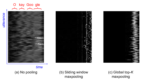
Fig. 5: Visualized attention weights for different pooling methods. In each image, x-axis is time, and y-axis is for different utterances in a training batch. (a) No pooling; (b) Sliding window maxpooling, where window size is 10, and step is 5; (c) Global top-$K$ maxpooling, where $K=5$.

5 Conclusions

In this paper, we experimented with different attention mechanisms for our keyword-based text-dependent speaker verification system [7]. From our experimental results, the best practice is to: (1) Use a shared-parameter non-linear scoring function; (2) Use a divided-layer attention connection to the last layer output of the LSTM; and (3) Apply a sliding window maxpooling on the attention weights. After combining all these best practices, we improved the EER of our baseline LSTM model from 1.72% to 1.48%, which is a 14% relative improvement. The same attention mechanisms, especially the ones using shared-parameter scoring functions, could potentially be used to improve text-independent speaker verification models [16] and speaker diarization systems [17].

References

- [1] Yury Pinsky, “Tomato, tomahto. google home now supports multiple users,” https://www.blog.google/products/assistant/tomato-tomahto-google-home-now-supports-multiple-users, 2017.
- [2] Mihai Matei, “Voice match will allow google home to recognize your voice,” https://www.androidheadlines.com/2017/10/voice-match-will-allow-google-home-to-recognize-your-voice.html, 2017.
- [3] Najim Dehak, Patrick J Kenny, Réda Dehak, Pierre Dumouchel, and Pierre Ouellet, “Front-end factor analysis for speaker verification,” IEEE Transactions on Audio, Speech, and Language Processing, vol. 19, no. 4, pp. 788–798, 2011.
- [4] Daniel Garcia-Romero and Carol Y Espy-Wilson, “Analysis of i-vector length normalization in speaker recognition systems.,” in Interspeech, 2011, pp. 249–252.
- [5] Yann LeCun, Yoshua Bengio, and Geoffrey Hinton, “Deep learning,” Nature, vol. 521, no. 7553, pp. 436–444, 2015.
- [6] Johan Rohdin, Anna Silnova, Mireia Diez, Oldrich Plchot, Pavel Matejka, and Lukas Burget, “End-to-end dnn based speaker recognition inspired by i-vector and plda,” arXiv preprint arXiv:1710.02369, 2017.
- [7] Georg Heigold, Ignacio Moreno, Samy Bengio, and Noam Shazeer, “End-to-end text-dependent speaker verification,” in Acoustics, Speech and Signal Processing (ICASSP), 2016 IEEE International Conference on. IEEE, 2016, pp. 5115–5119.
- [8] Sepp Hochreiter and Jürgen Schmidhuber, “Long short-term memory,” Neural computation, vol. 9, no. 8, pp. 1735–1780, 1997.
- [9] Guoguo Chen, Carolina Parada, and Georg Heigold, “Small-footprint keyword spotting using deep neural networks,” in Acoustics, Speech and Signal Processing (ICASSP), 2014 IEEE International Conference on. IEEE, 2014, pp. 4087–4091.
- [10] Rohit Prabhavalkar, Raziel Alvarez, Carolina Parada, Preetum Nakkiran, and Tara N Sainath, “Automatic gain control and multi-style training for robust small-footprint keyword spotting with deep neural networks,” in Acoustics, Speech and Signal Processing (ICASSP), 2015 IEEE International Conference on. IEEE, 2015, pp. 4704–4708.
- [11] Jan K Chorowski, Dzmitry Bahdanau, Dmitriy Serdyuk, Kyunghyun Cho, and Yoshua Bengio, “Attention-based models for speech recognition,” in Advances in Neural Information Processing Systems, 2015, pp. 577–585.
- [12] Minh-Thang Luong, Hieu Pham, and Christopher D Manning, “Effective approaches to attention-based neural machine translation,” arXiv preprint arXiv:1508.04025, 2015.
- [13] Kelvin Xu, Jimmy Ba, Ryan Kiros, Kyunghyun Cho, Aaron Courville, Ruslan Salakhudinov, Rich Zemel, and Yoshua Bengio, “Show, attend and tell: Neural image caption generation with visual attention,” in International Conference on Machine Learning, 2015, pp. 2048–2057.
- [14] Florian Schroff, Dmitry Kalenichenko, and James Philbin, “Facenet: A unified embedding for face recognition and clustering,” in Proceedings of the IEEE Conference on Computer Vision and Pattern Recognition, 2015, pp. 815–823.
- [15] Haşim Sak, Andrew Senior, and Françoise Beaufays, “Long short-term memory recurrent neural network architectures for large scale acoustic modeling,” in Fifteenth Annual Conference of the International Speech Communication Association, 2014.
- [16] Li Wan, Quan Wang, Alan Papir, and Ignacio Lopez Moreno, “Generalized end-to-end loss for speaker verification,” arXiv preprint arXiv:1710.10467, 2017.
- [17] Quan Wang, Carlton Downey, Li Wan, Philip Mansfield, and Ignacio Lopez Moreno, “Speaker diarization with lstm,” arXiv preprint arXiv:1710.10468, 2017.