Generalized End-to-End Loss for Speaker Verification

Abstract

In this paper, we propose a new loss function called generalized end-to-end (GE2E) loss, which makes the training of speaker verification models more efficient than our previous tuple-based end-to-end (TE2E) loss function. Unlike TE2E, the GE2E loss function updates the network in a way that emphasizes examples that are difficult to verify at each step of the training process. Additionally, the GE2E loss does not require an initial stage of example selection. With these properties, our model with the new loss function decreases speaker verification EER by more than $10\%$, while reducing the training time by $60\%$ at the same time. We also introduce the MultiReader technique, which allows us to do domain adaptation — training a more accurate model that supports multiple keywords (i.e., “OK Google” and “Hey Google”) as well as multiple dialects.

Index Terms—  Speaker verification, end-to-end loss, MultiReader, keyword detection

1 Introduction

1.1 Background

Speaker verification (SV) is the process of verifying whether an utterance belongs to a specific speaker, based on that speaker’s known utterances (i.e., enrollment utterances), with applications such as Voice Match [1, 2].

Depending on the restrictions of the utterances used for enrollment and verification, speaker verification models usually fall into one of two categories: text-dependent speaker verification (TD-SV) and text-independent speaker verification (TI-SV). In TD-SV, the transcript of both enrollment and verification utterances is phonetially constrained, while in TI-SV, there are no lexicon constraints on the transcript of the enrollment or verification utterances, exposing a larger variability of phonemes and utterance durations [3, 4]. In this work, we focus on TI-SV and a particular subtask of TD-SV known as global password TD-SV, where the verification is based on a detected keyword, e.g. “OK Google” [5, 6]

In previous studies, i-vector based systems have been the dominating approach for both TD-SV and TI-SV applications [7]. In recent years, more efforts have been focusing on using neural networks for speaker verification, while the most successful systems use end-to-end training [8, 9, 10, 11, 12]. In such systems, the neural network output vectors are usually referred to as embedding vectors (also known as d-vectors). Similarly to as in the case of i-vectors, such embedding can then be used to represent utterances in a fix dimensional space, in which other, typically simpler, methods can be used to disambiguate among speakers.

1.2 Tuple-Based End-to-End Loss

In our previous work [13], we proposed the tuple-based end-to-end (TE2E) model, which simulates the two-stage process of runtime enrollment and verification during training. In our experiments, the TE2E model combined with LSTM [14] achieved the best performance at the time. For each training step, a tuple of one evaluation utterance $\mathbf{x}_{j\sim}$ and $M$ enrollment utterances $\mathbf{x}_{km}$ (for $m=1,\dots,M$) is fed into our LSTM network: $\{\mathbf{x}_{j\sim},(\mathbf{x}_{k1},\dots,\mathbf{x}_{kM})\}$, where $\mathbf{x}$ represents the features (log-mel-filterbank energies) from a fixed-length segment, $j$ and $k$ represent the speakers of the utterances, and $j$ may or may not equal $k$. The tuple includes a single utterance from speaker $j$ and $M$ different utterance from speaker $k$. We call a tuple positive if ${\mathbf{x}}_{j\sim}$ and the $M$ enrollment utterances are from the same speaker, i.e., $j=k$, and negative otherwise. We generate positive and negative tuples alternatively.

For each input tuple, we compute the L2 normalized response of the LSTM: $\{\mathbf{e}_{j\sim},(\mathbf{e}_{k1},\dots,\mathbf{e}_{kM})\}$. Here each $\mathbf{e}$ is an embedding vector of fixed dimension that results from the sequence-to-vector mapping defined by the LSTM. The centroid of tuple $(\mathbf{e}_{k1},\dots,\mathbf{e}_{kM})$ represents the voiceprint built from $M$ utterances, and is defined as follows:

$$\mathbf{c}_{k}=\mathbb{E}_{m}[\mathbf{e}_{km}]=\frac{1}{M}\sum_{m=1}^{M}\mathbf{e}_{km}.$$ (1)

The similarity is defined using the cosine similarity function:

$$s=w\cdot\cos(\mathbf{e}_{j\sim},\mathbf{c}_{k})+b,$$ (2)

with learnable $w$ and $b$. The TE2E loss is finally defined as:

$$L_{\mathrm{T}}(\mathbf{e}_{j\sim},\mathbf{c}_{k})=\delta(j,k)\Big{(}1-\sigma(s)\Big{)}+\Big{(}1-\delta(j,k)\Big{)}\sigma(s).$$ (3)

Here $\sigma(x)=1/(1+e^{-x})$ is the standard sigmoid function and $\delta(j,k)$ equals $1$ if $j=k$, otherwise equals to $0$. The TE2E loss function encourages a larger value of $s$ when $k=j$, and a smaller value of $s$ when $k\neq j$. Consider the update for both positive and negative tuples — this loss function is very similar to the triplet loss in FaceNet [15].

1.3 Overview

In this paper, we introduce a generalization of our TE2E architecture. This new architecture constructs tuples from input sequences of various lengths in a more efficient way, leading to a significant boost of performance and training speed for both TD-SV and TI-SV. This paper is organized as follows: In Sec. 2.1 we give the definition of the GE2E loss; Sec. 2.2 is the theoretical justification for why GE2E updates the model parameters more effectively; Sec. 2.3 introduces a technique called “MultiReader”, which enables us to train a single model that supports multiple keywords and languages; Finally, we present our experimental results in Sec. 3.

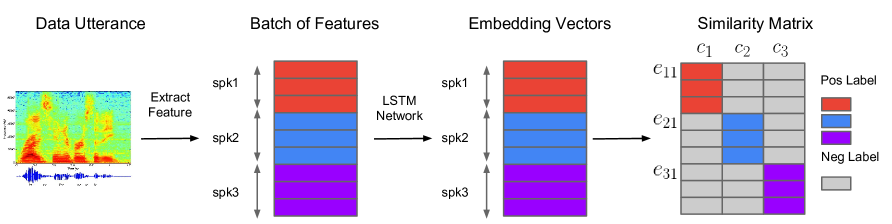
Fig. 1: System overview. Different colors indicate utterances/embeddings from different speakers.

2 Generalized End-to-End Model

Generalized end-to-end (GE2E) training is based on processing a large number of utterances at once, in the form of a batch that contains $N$ speakers, and $M$ utterances from each speaker in average, as is depicted in Figure 1.

2.1 Training Method

We fetch $N\times M$ utterances to build a batch. These utterances are from $N$ different speakers, and each speaker has $M$ utterances. Each feature vector $\mathbf{x}_{ji}$ ($1\leq j\leq N$ and $1\leq i\leq M$) represents the features extracted from speaker $j$ utterance $i$.

Similar to our previous work [13], we feed the features extracted from each utterance $\mathbf{x}_{ji}$ into an LSTM network. A linear layer is connected to the last LSTM layer as an additional transformation of the last frame response of the network. We denote the output of the entire neural network as $f(\mathbf{x}_{ji};\mathbf{w})$ where $\mathbf{w}$ represents all parameters of the neural network (including both, LSTM layers and the linear layer). The embedding vector (d-vector) is defined as the L2 normalization of the network output:

$$\mathbf{e}_{ji}=\frac{f(\mathbf{x}_{ji};\mathbf{w})}{||f(\mathbf{x}_{ji};\mathbf{w})||_{2}}.$$ (4)

Here $\mathbf{e}_{ji}$ represents the embedding vector of the $j$th speaker’s $i$th utterance. The centroid of the embedding vectors from the $j$th speaker $[\mathbf{e}_{j1},\dots,\mathbf{e}_{jM}]$ is defined as $\mathbf{c}_{j}$ via Equation 1.

The similarity matrix $\mathbf{S}_{ji,k}$ is defined as the scaled cosine similarities between each embedding vector $\mathbf{e}_{ji}$ to all centroids $\mathbf{c}_{k}$ ($1\leq j,k\leq N$, and $1\leq i\leq M$):

$$\mathbf{S}_{ji,k}=w\cdot\cos(\mathbf{e}_{ji},\mathbf{c}_{k})+b,$$ (5)

where $w$ and $b$ are learnable parameters. We constrain the weight to be positive $w>0$, because we want the similarity to be larger when cosine similarity is larger. The major difference between TE2E and GE2E is as follows:

• TE2E’s similarity (Equation 2) is a scalar value that defines the similarity between embedding vector $\mathbf{e}_{j\sim}$ and a single tuple centroid $\mathbf{c}_{k}$.

• GE2E builds a similarity matrix (Equation 5) that defines the similarities between each $\mathbf{e}_{ji}$ and all centroids $\mathbf{c}_{k}$.

Figure 1 illustrates the whole process with features, embedding vectors, and similarity scores from different speakers, represented by different colors.

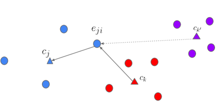
Fig. 2: GE2E loss pushes the embedding towards the centroid of the true speaker, and away from the centroid of the most similar different speaker.

During the training, we want the embedding of each utterance to be similar to the centroid of all that speaker’s embeddings, while at the same time, far from other speakers’ centroids. As shown in the similarity matrix in Figure 1, we want the similarity values of colored areas to be large, and the values of gray areas to be small. Figure 2 illustrates the same concept in a different way: we want the blue embedding vector to be close to its own speaker’s centroid (blue triangle), and far from the others centroids (red and purple triangles), especially the closest one (red triangle). Given an embedding vector $\mathbf{e}_{ji}$, all centroids $\mathbf{c}_{k}$, and the corresponding similarity matrix $\mathbf{S}_{ji,k}$, there are two ways to implement this concept:

Softmax We put a softmax on $\mathbf{S}_{ji,k}$ for $k=1,\dots,N$ that makes the output equal to $1$ iff $k=j$, otherwise makes the output equal to $0$. Thus, the loss on each embedding vector $\mathbf{e}_{ji}$ could be defined as:

$$L(\mathbf{e}_{ji})=-\mathbf{S}_{ji,j}+\log\sum_{k=1}^{N}\exp(\mathbf{S}_{ji,k}).$$ (6)

This loss function means that we push each embedding vector close to its centroid and pull it away from all other centroids.

Contrast The contrast loss is defined on positive pairs and most aggressive negative pairs, as:

$$L(\mathbf{e}_{ji})=1-\sigma(\mathbf{S}_{ji,j})+\max_{\begin{subarray}{c}1\leq k\leq N\\ k\neq j\end{subarray}}\sigma(\mathbf{S}_{ji,k}),$$ (7)

where $\sigma(x)=1/(1+e^{-x})$ is the sigmoid function. For every utterance, exactly two components are added to the loss: (1) A positive component, which is associated with a positive match between the embedding vector and its true speaker’s voiceprint (centroid). (2) A hard negative component, which is associated with a negative match between the embedding vector and the voiceprint (centroid) with the highest similarity among all false speakers.

In Figure 2, the positive term corresponds to pushing $\mathbf{e}_{ji}$ (blue circle) towards $\mathbf{c}_{j}$ (blue triangle). The negative term corresponds to pulling $\mathbf{e}_{ji}$ (blue circle) away from $\mathbf{c}_{k}$ (red triangle), because $\mathbf{c}_{k}$ is more similar to $\mathbf{e}_{ji}$ compared with $\mathbf{c}_{k^{\prime}}$. Thus, contrast loss allows us to focus on difficult pairs of embedding vector and negative centroid.

In our experiments, we find both implementations of GE2E loss are useful: contrast loss performs better for TD-SV, while softmax loss performs slightly better for TI-SV.

In addition, we observed that removing $\mathbf{e}_{ji}$ when computing the centroid of the true speaker makes training stable and helps avoid trivial solutions. So, while we still use Equation 1 when calculating negative similarity (i.e., $k\neq j$), we instead use Equation 8 when $k=j$:

$$\mathbf{c}_{j}^{(-i)} = \frac{1}{M-1}\sum_{\begin{subarray}{c}m=1\\ m\neq i\end{subarray}}^{M}\mathbf{e}_{jm},$$ (8)

$$\mathbf{S}_{ji,k} = \begin{cases}w\cdot\cos(\mathbf{e}_{ji},\mathbf{c}_{j}^{(-i)})+b&\text{if}\quad k=j;\\ w\cdot\cos(\mathbf{e}_{ji},\mathbf{c}_{k})+b&\text{otherwise}.\end{cases}$$ (9)

Combining Equations 4, 6, 7 and 9, the final GE2E loss $L_{G}$ is the sum of all losses over the similarity matrix ($1\leq j\leq N$, and $1\leq i\leq M$):

$$L_{G}(\mathbf{x};\mathbf{w})=L_{G}(\mathbf{S})=\sum_{j,i}L(\mathbf{e}_{ji}).$$ (10)

2.2 Comparison between TE2E and GE2E

Consider a single batch in GE2E loss update: we have $N$ speakers, each with $M$ utterances. Each single step update will push all $N\times M$ embedding vectors toward their own centroids, and pull them away the other centroids.

This mirrors what happens with all possible tuples in the TE2E loss function [13] for each $\mathbf{x}_{ji}$. Assume we randomly choose $P$ utterances from speaker $j$ when comparing speakers:

1. Positive tuples: $\{\mathbf{x}_{ji},(\mathbf{x}_{j,i_{1}},\dots,\mathbf{x}_{j,i_{P}})\}$ for $1\leq i_{p}\leq M$ and $p=1,\dots,P$. There are $\binom{M}{P}$ such positive tuples.

2. Negative tuples: $\{\mathbf{x}_{ji},(\mathbf{x}_{k,i_{1}},\dots,\mathbf{x}_{k,i_{P}})\}$ for $k\neq j$ and $1\leq i_{p}\leq M$ for $p=1,\ldots,P$. For each $\mathbf{x}_{ji}$, we have to compare with all other $N-1$ centroids, where each set of those $N-1$ comparisons contains $\binom{M}{P}$ tuples.

Each positive tuple is balanced with a negative tuple, thus the total number is the maximum number of positive and negative tuples times 2. So, the total number of tuples in TE2E loss is:

$$2\times\max\Big{(}\binom{M}{P},(N-1)\binom{M}{P}\Big{)}\geq 2(N-1).$$ (11)

The lower bound of Equation 11 occurs when $P=M$. Thus, each update for $\mathbf{x}_{ji}$ in our GE2E loss is identical to at least $2(N-1)$ steps in our TE2E loss. The above analysis shows why GE2E updates models more efficiently than TE2E, which is consistent with our empirical observations: GE2E converges to a better model in shorter time (See Sec. 3 for details).

2.3 Training with MultiReader

Consider the following case: we care about the model application in a domain with a small dataset $D_{1}$. At the same time, we have a larger dataset $D_{2}$ in a similar, but not identical domain. We want to train a single model that performs well on dataset $D_{1}$, with the help from $D_{2}$:

$$L(D_{1},D_{2};\mathbf{w})=\mathbb{E}_{x\in D_{1}}[L(\mathbf{x};\mathbf{w})]+\alpha\mathbb{E}_{x\in D_{2}}[L(\mathbf{x};\mathbf{w})].$$ (12)

This is similar to the regularization technique: in normal regularization, we use $\alpha||\mathbf{w}||_{2}^{2}$ to regularize the model. But here, we use $\mathbb{E}_{x\in D_{2}}[L(\mathbf{x};\mathbf{w})]$ for regularization. When dataset $D_{1}$ does not have sufficient data, training the network on $D_{1}$ can lead to overfitting. Requiring the network to also perform reasonably well on $D_{2}$ helps to regularize the network.

This can be generalized to combine $K$ different, possibly extremely unbalanced, data sources: $D_{1},\dots,D_{K}$. We assign a weight $\alpha_{k}$ to each data source, indicating the importance of that data source. During training, in each step we fetch one batch/tuple of utterances from each data source, and compute the combined loss as: $L(D_{1},\cdots,D_{K})=\sum_{k=1}^{K}\alpha_{k}\mathbb{E}_{\mathbf{x}_{k}\in D_{k}}[L(\mathbf{x}_{k};\mathbf{w})]$, where each $L(\mathbf{x}_{k};w)$ is the loss defined in Equation 10.

3 Experiments

In our experiments, the feature extraction process is the same as [6]. The audio signals are first transformed into frames of width 25ms and step 10ms. Then we extract 40-dimension log-mel-filterbank energies as the features for each frame. For TD-SV applications, the same features are used for both keyword detection and speaker verification. The keyword detection system will only pass the frames containing the keyword into the speaker verification system. These frames form a fixed-length (usually 800ms) segment. For TI-SV applications, we usually extract random fixed-length segments after Voice Activity Detection (VAD), and use a sliding window approach for inference (discussed in Sec. 3.2) .

Our production system uses a 3-layer LSTM with projection [16]. The embedding vector (d-vector) size is the same as the LSTM projection size. For TD-SV, we use $128$ hidden nodes and the projection size is $64$. For TI-SV, we use $768$ hidden nodes with projection size $256$. When training the GE2E model, each batch contains $N=64$ speakers and $M=10$ utterances per speaker. We train the network with SGD using initial learning rate $0.01$, and decrease it by half every 30M steps. The L2-norm of gradient is clipped at $3$ [17], and the gradient scale for projection node in LSTM is set to $0.5$. Regarding the scaling factor $(w,b)$ in loss function, we also observed that a good initial value is $(w,b)=(10,-5)$, and the smaller gradient scale of $0.01$ on them helped to smooth convergence.

3.1 Text-Dependent Speaker Verification

Though existing voice assistants usually only support a single keyword, studies show that users prefer that multiple keywords are supported at the same time. For multi-user on Google Home, two keywords are supported simultaneously: “OK Google” and “Hey Google”.

Enabling speaker verification on multiple keywords falls between TD-SV and TI-SV, since the transcript is neither constrained to a single phrase, nor completely unconstrained. We solve this problem using the MultiReader technique (Sec. 2.3). MultiReader has a great advantage compared to simpler approaches, e.g. directly mixing multiple data sources together: It handles the case when different data sources are unbalanced in size. In our case, we have two data sources for training: 1) An “OK Google” training set from anonymized user queries with $\sim 150$ M utterances and $\sim 630$ K speakers; 2) A mixed “OK/Hey Google” training set that is manually collected with $\sim 1.2$ M utterances and $\sim 18$ K speakers. The first dataset is larger than the second by a factor of 125 in the number of utterances and 35 in the number of speakers.

For evaluation, we report the Equal Error Rate (EER) on four cases: enroll with either keyword, and verify on either keyword. All evaluation datasets are manually collected from 665 speakers with an average of $4.5$ enrollment utterances and $10$ evaluation utterances per speaker. The results are shown in Table 1. As we can see, MultiReader brings around 30% relative improvement on all four cases.

Table 1: MultiReader vs. directly mixing multiple data sources.

Test data	Mixed data	MultiReader
(Enroll $\rightarrow$ Verify)	EER (%)	EER (%)
OK Google $\rightarrow$ OK Google	1.16	0.82
OK Google $\rightarrow$ Hey Google	4.47	2.99
Hey Google $\rightarrow$ OK Google	3.30	2.30
Hey Google $\rightarrow$ Hey Google	1.69	1.15

We also performed more comprehensive evaluations in a larger dataset collected from $\sim 83$ K different speakers and environmental conditions, from both anonymized logs and manual collections. We use an average of $7.3$ enrollment utterances and $5$ evaluation utterances per speaker. Table 2 summarizes average EER for different loss functions trained with and without MultiReader setup. The baseline model is a single layer LSTM with $512$ nodes and an embedding vector size of $128$ [13]. The second and third rows’ model architecture is 3-layer LSTM. Comparing the 2nd and 3rd rows, we see that GE2E is about $10\%$ better than TE2E. Similar to Table 1, here we also see that the model performs significantly better with MultiReader. While not shown in the table, it is also worth noting that the GE2E model took about $60\%$ less training time than TE2E.

Table 2: Text-dependent speaker verification EER.

Model	Embed	Loss	Multi	Average
Architecture	Size		Reader	EER (%)
$(512,)$ [13]	$128$	TE2E	No	3.30
			Yes	2.78
$(128,64)\times 3$	$64$	TE2E	No	3.55
			Yes	2.67
$(128,64)\times 3$	$64$	GE2E	No	3.10
			Yes	2.38

3.2 Text-Independent Speaker Verification

For TI-SV training, we divide training utterances into smaller segments, which we refer to as partial utterances. While we don’t require all partial utterances to be of the same length, all partial utterances in the same batch must be of the same length. Thus, for each batch of data, we randomly choose a time length $t$ within $[lb,ub]=[140,180]$ frames, and enforce that all partial utterances in that batch are of length $t$ (as shown in Figure 3).

During inference time, for every utterance we apply a sliding window of fixed size $(lb+ub)/2=160$ frames with $50\%$ overlap. We compute the d-vector for each window. The final utterance-wise d-vector is generated by L2 normalizing the window-wise d-vectors, then taking the element-wise averge (as shown in Figure 4).

Our TI-SV models are trained on around 36M utterances from 18K speakers, which are extracted from anonymized logs. For evaluation, we use an additional 1000 speakers with in average 6.3 enrollment utterances and 7.2 evaluation utterances per speaker. Table 3 shows the performance comparison between different training loss functions. The first column is a softmax that predicts the speaker label for all speakers in the training data. The second column is a model trained with TE2E loss. The third column is a model trained with GE2E loss. As shown in the table, GE2E performs better than both softmax and TE2E. The EER performance improvement is larger than $10\%$. In addition, we also observed that GE2E training was about $3\times$ faster than the other loss functions.

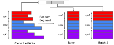
Fig. 3: Batch construction process for training TI-SV models.

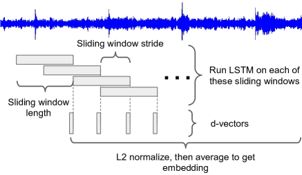
Fig. 4: Sliding window used for TI-SV.

Table 3: Text-independent speaker verification EER (%).

Softmax	TE2E [13]	GE2E
4.06	4.13	3.55

4 Conclusions

In this paper, we proposed the generalized end-to-end (GE2E) loss function to train speaker verification models more efficiently. Both theoretical and experimental results verified the advantage of this novel loss function. We also introduced the MultiReader technique to combine different data sources, enabling our models to support multiple keywords and multiple languages. By combining these two techniques, we produced more accurate speaker verification models.

References

- [1] Yury Pinsky, “Tomato, tomahto. Google Home now supports multiple users,” https://www.blog.google/products/assistant/tomato-tomahto-google-home-now-supports-multiple-users, 2017.
- [2] Mihai Matei, “Voice match will allow Google Home to recognize your voice,” https://www.androidheadlines.com/2017/10/voice-match-will-allow-google-home-to-recognize-your-voice.html, 2017.
- [3] Tomi Kinnunen and Haizhou Li, “An overview of text-independent speaker recognition: From features to supervectors,” Speech communication, vol. 52, no. 1, pp. 12–40, 2010.
- [4] Frédéric Bimbot, Jean-François Bonastre, Corinne Fredouille, Guillaume Gravier, Ivan Magrin-Chagnolleau, Sylvain Meignier, Teva Merlin, Javier Ortega-García, Dijana Petrovska-Delacrétaz, and Douglas A Reynolds, “A tutorial on text-independent speaker verification,” EURASIP journal on applied signal processing, vol. 2004, pp. 430–451, 2004.
- [5] Guoguo Chen, Carolina Parada, and Georg Heigold, “Small-footprint keyword spotting using deep neural networks,” in Acoustics, Speech and Signal Processing (ICASSP), 2014 IEEE International Conference on. IEEE, 2014, pp. 4087–4091.
- [6] Rohit Prabhavalkar, Raziel Alvarez, Carolina Parada, Preetum Nakkiran, and Tara N Sainath, “Automatic gain control and multi-style training for robust small-footprint keyword spotting with deep neural networks,” in Acoustics, Speech and Signal Processing (ICASSP), 2015 IEEE International Conference on. IEEE, 2015, pp. 4704–4708.
- [7] Najim Dehak, Patrick J Kenny, Réda Dehak, Pierre Dumouchel, and Pierre Ouellet, “Front-end factor analysis for speaker verification,” IEEE Transactions on Audio, Speech, and Language Processing, vol. 19, no. 4, pp. 788–798, 2011.
- [8] Ehsan Variani, Xin Lei, Erik McDermott, Ignacio Lopez Moreno, and Javier Gonzalez-Dominguez, “Deep neural networks for small footprint text-dependent speaker verification,” in Acoustics, Speech and Signal Processing (ICASSP), 2014 IEEE International Conference on. IEEE, 2014, pp. 4052–4056.
- [9] Yu-hsin Chen, Ignacio Lopez-Moreno, Tara N Sainath, Mirkó Visontai, Raziel Alvarez, and Carolina Parada, “Locally-connected and convolutional neural networks for small footprint speaker recognition,” in Sixteenth Annual Conference of the International Speech Communication Association, 2015.
- [10] Chao Li, Xiaokong Ma, Bing Jiang, Xiangang Li, Xuewei Zhang, Xiao Liu, Ying Cao, Ajay Kannan, and Zhenyao Zhu, “Deep speaker: an end-to-end neural speaker embedding system,” CoRR, vol. abs/1705.02304, 2017.
- [11] Shi-Xiong Zhang, Zhuo Chen, Yong Zhao, Jinyu Li, and Yifan Gong, “End-to-end attention based text-dependent speaker verification,” CoRR, vol. abs/1701.00562, 2017.
- [12] Seyed Omid Sadjadi, Sriram Ganapathy, and Jason W. Pelecanos, “The IBM 2016 speaker recognition system,” CoRR, vol. abs/1602.07291, 2016.
- [13] Georg Heigold, Ignacio Moreno, Samy Bengio, and Noam Shazeer, “End-to-end text-dependent speaker verification,” in Acoustics, Speech and Signal Processing (ICASSP), 2016 IEEE International Conference on. IEEE, 2016, pp. 5115–5119.
- [14] Sepp Hochreiter and Jürgen Schmidhuber, “Long short-term memory,” Neural computation, vol. 9, no. 8, pp. 1735–1780, 1997.
- [15] Florian Schroff, Dmitry Kalenichenko, and James Philbin, “Facenet: A unified embedding for face recognition and clustering,” in Proceedings of the IEEE Conference on Computer Vision and Pattern Recognition, 2015, pp. 815–823.
- [16] Haşim Sak, Andrew Senior, and Françoise Beaufays, “Long short-term memory recurrent neural network architectures for large scale acoustic modeling,” in Fifteenth Annual Conference of the International Speech Communication Association, 2014.
- [17] Razvan Pascanu, Tomas Mikolov, and Yoshua Bengio, “Understanding the exploding gradient problem,” CoRR, vol. abs/1211.5063, 2012.