Criticality and hidden criticality in multi-species Bose-Einstein condensates

Abstract

A general approach is proposed to solve the coupled Gross-Pitaevskii equations (CGP) for K-species Bose-Einstein condensates (BEC). Analytical solutions have been obtained under the Thomas-Fermi approximation. We aim at finding out the common features of the K-species BEC. In particular, two types of phase-transitions, full-state-transition and partial-state transition, are found. In the former all species are involved in the transition, while in the latter only a few specified species are essentially involved. This leads to the criticality and the hidden criticality (previously found in multi-band superconductivity). We further found that the former originates from the singularity of the whole matrix of the CGP, while the latter originates from the singularity of a specified sub-matrix (which is contributed by only a few specified species). It is emphasized that the singularity is not a by-product of the TFA, but is inherent in the CGP.

I Introduction

The Bose-Einstein condensates (BEC) are artificial and controllable many-body systems. In principle, their behavior can be designed. Therefore, these systems are very valuable in both academic and practical senses. The research into the 2-species BEC was initiated in 1996. Since then, an increasing effort is paid in both the experimental aspect myat97 ; ande05 ; ni08 ; pilc09 ; nemi09 ; wack15 ; mgr and theoretical aspectho96 ; esry97 ; pu98 ; chui99 ; tripp00 ; ribo02 ; chui03 ; luo07 ; luo08 ; nott15 ; scha15 ; inde15 ; kuop15 ; polo15 ; jsy ; mpe ; rci ; jpb . During the progress a noticeable point is the relation between the BEC and other many-body systems. Recently, the similarity on the criticality and the hidden criticality between the multi-species BEC and the multi-band superconductivity was primary found sr ; sup1 ; sup2 ; sup3 ; sup4 . It is believed that new and rich physical phenomena would emerge from multi-species BEC. Some of them and those found in other many-body systems might have the same physical background. Thus the knowledge extracted from the multi-species BEC would be in general helpful for understanding the behavior of other many-body systems. Moreover, multi-species BEC is experimentally realizable. Thus, the study of this topic is meaningful and practical. In fact, the study on 3-species BEC has already been initiated cal ; man ; orl ; v2 .

This paper is one along this line. it is a generalization of our two previous paper jpa ; sr from three-species BEC to K-species, and from adopting a spherical-symmetric trap to a more general trap (spherical- and axial-symmetric traps are considered as special cases). The aim is to find out the common features existing in various multi-species BEC. The emphasis is placed on the qualitative aspect and on the critical phenomena. For this purpose, we have to solve the coupled Gross-Pitaevskii equations (CGP) to obtain the solution for the ground states. It is assumed that the particle numbers are huge so that the Thomas-Fermi approximation (TFA) is reasonable and therefore can be adopted. Under the TFA, an approach is proposed so that the solutions are obtained with an analytical form. The analytical formalism facilitate greatly the related analysis so that the inherent physics can be better understood.

II Coupled Gross-pitaevskii equations and the formal solutions

There are $N_{I}$ I-th-atoms, each has mass $m_{I}$ and they are interacting via $V_{I}=c_{I,I}\underset{1\leq i<i^{\prime}\leq N_{I}}{\Sigma}\delta(\mathbf{r}_{i}-\mathbf{r}_{i^{\prime}})$, where $I$ is from 1 to $K(\geq 2)$. All the particle numbers $N_{I}$ are assumed to be huge (say, $\geq$10000). The interspecies interactions are $V_{IJ}=c_{I,J}\underset{1\leq i\leq N_{I}}{\Sigma}\cdot\underset{1\leq j\leq N_{J}}{\Sigma}\delta(\mathbf{r}_{i}-\mathbf{r}_{j})$. These atoms are confined by 3-D harmonic traps $\frac{1}{2}m_{I}(\omega_{Ix}^{2}x^{2}+\omega_{Iy}^{2}y^{2}+\omega_{Iz}^{2}z^{2})$. We introduce a mass $m$ and a frequency $\omega$. Then, $\hbar\omega$ and $\lambda\equiv\sqrt{\hbar/(m\omega)}$ are used as units for energy and length. The spin degrees of freedom are considered as being frozen. The total Hamiltonian is

$$H = \underset{1\leq I\leq K}{\Sigma}H_{I}+\underset{1\leq I<J\leq K}{\Sigma}V_{IJ}$$

$$H_{I} = \sum_{i=1}^{N_{I}}[-\frac{m}{2m_{I}}\nabla_{i}^{2}+\frac{1}{2}(\gamma_{Ix}x_{i}^{2}+\gamma_{Iy}y_{i}^{2}+\gamma_{Iz}z_{i}^{2})]$$ (2)

$$+V_{I}$$

where $\gamma_{Il}=(m_{I}/m)(\omega_{Il}/\omega)^{2}$, $l=x$, $y$, or $z$ (the same in the follows).

We are interested in the g.s. where no spatial excitations are involved, and each kind of atoms are fully condensed into a state which is most advantageous for binding. Accordingly, the total many-body wave function of the g.s. can be written as

$$\Psi=\prod_{i_{1}=1}^{N_{1}}\phi_{1}(\mathbf{r}_{i_{1}})\cdot\cdot\cdot\cdot\prod_{i_{K}=1}^{N_{K}}\phi_{K}(\mathbf{r}_{i_{K}})$$ (3)

where $\phi_{I}(\mathbf{r})$ is the normalized single particle wave function. The associated CGP is a set of K coupled equations. The I-th of them is

$$[-\frac{m}{2m_{I}}\nabla^{2}+\frac{1}{2}\Sigma_{l}\gamma_{Il}l^{2}+\underset{1\leq J\leq K}{\Sigma}\alpha_{IJ}\phi_{J}^{2}-\varepsilon_{I}]\phi_{I}=0$$ (4)

where the summation of $l$ covers $x$, $y$, and $z$. $\alpha_{IJ}\equiv N_{J}c_{I,J}$ and is called the weighted strength (W-strength). $\varepsilon_{I}$ is the chemical potential. It is emphasized that the normalization ${\int\phi_{l}^{2}d\mathbf{r}=1}$ is required.

Since the total kinetic energy is proportional to the total particle numbers $N$ while the total interaction energy is $\propto N^{2}$, the relative importance of the former becomes very small when $N$ becomes very large. In this case, TFA (neglect the kinetic energies) can be adopted. The applicability of this approximation has been evaluated via a numerical approach given in yzhe ; polo15 . Under the TFA and in a specific spatial domain where all the $\phi_{I}$ ($I$ from 1 to $K$) are nonzero, the CGP can be written in a matrix form as

$$\mathfrak{[\alpha}_{IJ}\mathfrak{]}\left(\begin{array}[]{c}\phi_{1}^{2}\\ \cdot\\ \cdot\\ \phi_{K}^{2}\end{array}\right)=\left(\begin{array}[]{c}\varepsilon_{1}-\frac{1}{2}\Sigma_{l}\gamma_{1l}l^{2}\\ \cdot\\ \cdot\\ \varepsilon_{K}-\frac{1}{2}\Sigma_{l}\gamma_{Kl}l^{2}\end{array}\right)$$ (5)

where $[\alpha_{IJ}]$ denotes a K-rank matrix with elements $\alpha_{IJ}$. When $[\alpha_{IJ}]$ is nonsingular, its reverse $[\alpha_{IJ}]^{-1}$ exists. Then we have a formal solution for $\{\phi\}$ as

$$\phi_{I}^{2}=X_{I}-\Sigma_{l}Y_{I,l}l^{2}$$ (6)

where $I$ is from 1 to $K$,

$$X_{I}=D_{X_{I}}/D$$ (7)

$D$ is the determinant of $[\alpha_{IJ}]$. $D_{X_{I}}$ is a determinant obtained by changing the $I-th$ column of $D$ from $(\alpha_{1I},\cdot\cdot\cdot\alpha_{KI})$ to $(\varepsilon_{1},\cdot\cdot\cdot\varepsilon_{K})$.

$$Y_{I,l}=D_{Y_{Il}}/D$$ (8)

$D_{Y_{Il}}$ is also a determinant obtained by changing the $I-th$ column of $D$ to $(\frac{1}{2}\gamma_{1l},\cdot\cdot\cdot\frac{1}{2}\gamma_{Kl})$. The set of $K$ wave functions given by eq.(6) is denoted as $\{\phi\}$ and is called a formal solution in Form K. From the reverse of eq.(7), we have a useful relation as

$$\varepsilon_{J}=\Sigma_{I}\alpha_{JI}X_{I}$$ (9)

If in a specific spatial domain only $K^{\prime}$ $(<K)$ wave functions are nonzero, then we define a subset $\sigma^{\prime}$ of the indexes so that all $\phi_{I^{\prime}}\geq 0$ ($I^{\prime}\in\sigma^{\prime}$) and all $\phi_{J^{\prime}}=0$ ($J^{\prime}\notin\sigma^{\prime}$). For the subset $\sigma^{\prime}$ with the species number $K^{\prime}$, the associated CGP can be written as

$$\mathfrak{[\alpha}_{I^{\prime}I"}\mathfrak{]}\left(\begin{array}[]{c}\phi_{1^{\prime}}^{2}\\ \cdot\\ \cdot\\ \phi_{K^{\prime}}^{2}\end{array}\right)=\left(\begin{array}[]{c}\varepsilon_{1^{\prime}}-\frac{1}{2}\Sigma_{l}\gamma_{1^{\prime}l}l^{2}\\ \cdot\\ \cdot\\ \varepsilon_{K^{\prime}}-\frac{1}{2}\Sigma_{l}\gamma_{K^{\prime}l}l^{2}\end{array}\right)$$ (10)

where $[\mathfrak{\alpha}_{I^{\prime}I"}]$ denotes a $K^{\prime}$-rank matrix with elements $\alpha_{I^{\prime}I"}$ (both $I^{\prime}$ and $I"\in\sigma^{\prime}$ ), and $1^{\prime}$ to $K^{\prime}$ denote the indexes in $\sigma^{\prime}$. When $[\mathfrak{\alpha}_{I^{\prime}I"}]$ is nonsingular, we have a formal solution as

$$(\phi_{I^{\prime}}^{\sigma^{\prime}})^{2}=X_{I^{\prime}}^{\sigma^{\prime}}-\Sigma_{l}Y_{I^{\prime}l}^{\sigma^{\prime}}l^{2}(\phi_{J^{\prime}}^{\sigma^{\prime}})^{2} = 0$$ (11)

$$(\phi_{J^{\prime}}^{\sigma^{\prime}})^{2} = 0$$ (12)

where

$$X_{I^{\prime}}^{\sigma^{\prime}}=D_{\sigma^{\prime},X_{I^{\prime}}}/D_{\sigma^{\prime}}$$ (13)

$D_{\sigma^{\prime}}$ is the determinant of $[\mathfrak{\alpha}_{I^{\prime}I"}]$. $D_{\sigma^{\prime},X_{I^{\prime}}}$ is a determinant obtained by changing the $I^{\prime}-th$ column of $D_{\sigma^{\prime}}$ from $(\alpha_{1^{\prime}I^{\prime}},\cdot\cdot\cdot\alpha_{K^{\prime}I^{\prime}})$ to $(\varepsilon_{1^{\prime}},\cdot\cdot\cdot\varepsilon_{K^{\prime}})$.

$$Y_{I^{\prime}l}^{\sigma^{\prime}}=D_{\sigma^{\prime},Y_{I^{\prime}l}}/D_{\sigma^{\prime}}$$ (14)

$D_{\sigma^{\prime},Y_{I^{\prime}l}}$ is also a determinant obtained by changing the $I^{\prime}-th$ column of $D_{\sigma^{\prime}}$ to $(\frac{1}{2}\gamma_{1^{\prime}l},\cdot\cdot\cdot\frac{1}{2}\gamma_{K^{\prime}l})$. The set of $K$ wave functions given by eq.(11) are denoted as $\{\phi^{\sigma^{\prime}}\}$, and is called a formal solution in Form $\sigma^{\prime}$.

From eq.(13) we obtain a useful formula

$$\varepsilon_{J^{\prime}}=\Sigma_{I^{\prime}}\alpha_{J^{\prime}I^{\prime}}X_{I^{\prime}}^{\sigma^{\prime}}$$ (15)

where $I^{\prime}\in\sigma^{\prime}$ and $J^{\prime}\in\sigma^{\prime}$.

Note that all the coefficients $Y_{I^{\prime}l}^{\sigma^{\prime}}$ involved in the formal solutions are completely determined by the parameters $\gamma_{I^{\prime}l}$ and $\alpha_{I^{\prime}J^{\prime}}$. When $Y_{I^{\prime}l}^{\sigma^{\prime}}$ is positive (negative), $\phi_{I^{\prime}}^{\sigma^{\prime}}$ must descend (rise up) when $l$ increases. Thus their signs are crucial to the behavior of the wave functions.

If in a domain only one wave function, say, $\phi_{I^{\prime\prime}}$, is nonzero, then, from eq.(4) (with the kinetic term removed), it is straight forward to obtain

$$\phi_{I^{{}^{\prime\prime}}}^{2}=\frac{1}{\alpha_{I^{\prime\prime}I^{\prime\prime}}}(\varepsilon_{I^{\prime\prime}}-\frac{1}{2}\Sigma_{l}\gamma_{I^{\prime\prime}l}l^{2})$$ (16)

while all the other wave functions are zero. This solution is called a formal solution in Form $1(I^{\prime\prime})$.

In what follows we shall see that these formal solutions, each hold in a specific domain, will act as building blocks and will link up to form an entire solution of the CGP.

III Two features of the formal solutions

There are two features important to the linking of the formal solutions

Feature I: Continuity in the linking

Let $P$ denotes a spatial point (or a group of points, say, a curve). Let us introduce the notation $\{\phi^{\sigma^{\prime}}\}_{P}$ which implies that the set of $K$ wave functions are all evaluated at $P$. Let $\{\sigma^{\prime}+J^{\prime}\}$ denotes an enlarged set including all the indexes in $\sigma^{\prime}$ together with an extra index $J^{\prime}\notin\sigma^{\prime}$. Then, for the point(s) $P$ where $\phi_{J^{\prime}}^{\{\sigma^{\prime}+J^{\prime}\}}=0$, we can prove that $\{\phi^{\{\sigma^{\prime}+J^{\prime}\}}\}_{P}=\{\phi^{\sigma^{\prime}}\}_{P}$ (namely, for any index $I$ (from 1 to $K$), $\phi_{I}^{\{\sigma^{\prime}+J^{\prime}\}}|_{P}=\phi_{I}^{\sigma^{\prime}}|_{P}$ holds ,i.e., the two sets of wave functions are one-by-one equal at $P$). This is because the two sets of equations for $\{\phi^{\{\sigma^{\prime}+J^{\prime}\}}\}$ and $\{\phi^{\sigma^{\prime}}\}$, respectively, will become the same at $P$ (refer to eq.(10)). Thus, when the Form $\sigma^{\prime}$ is transformed to $\{\sigma^{\prime}+J^{\prime}\}$ at $P$, all the wave functions remain to be continuous.

Feature II: When the coordinate moves along a direction, at least one of the nonzero wave functions are descending

This common feature holds when all the interactions are repulsive. The proof is as follows.

From eq.(10) we know that the Form $\sigma^{\prime}$ could exist only if the matrix $[\alpha_{I^{\prime}J^{\prime}}]$ is nonsingular. Therefore, when each of its column is considered as a vector, the column vectors are linearly independent. Thus, the vector $(\gamma_{1^{\prime}l},\cdot\cdot\cdot\gamma_{K^{\prime}l})$ can be in general expanded as

$$\left(\begin{array}[]{c}\gamma_{1^{\prime}l}\\ \cdot\\ \cdot\\ \gamma_{K^{\prime}l}\end{array}\right)=\underset{J^{\prime}}{\Sigma}\eta_{J^{\prime}}^{(l)}\left(\begin{array}[]{c}\alpha_{1^{\prime}J^{\prime}}\\ \cdot\\ \cdot\\ \alpha_{K^{\prime}J^{\prime}}\end{array}\right)$$ (17)

In Insert this equation into $D_{\sigma^{\prime},Y_{I^{\prime}l}}$, then we have $Y_{I^{\prime}l}=\eta_{I^{\prime}}^{(l)}/2$. When all the interactions are repulsive, all the matrix elements $\{\alpha_{I^{\prime}J^{\prime}}\}$ are positive. Furthermore, all the $\gamma_{I^{\prime}l}$ are also positive due to their definitions. Thus, when all the $\eta_{I^{\prime}}^{(l)}$ were negative, eq.(17) would lead to a contradiction. Thus, for any $\sigma^{\prime}$ and $l$, $Y_{I^{\prime}l}^{\sigma^{\prime}}$ ($I^{\prime}\in\sigma^{\prime}$) can not all be negative. It implies that at least one of them is positive. Accordingly, at least one of the wave functions are descending when $l$ increases, thus this feature is proved.

The Feature II has profound influence on the behavior of the solutions of the CGP. For any formal solution at least one of the nonzero wave functions will descend along a given direction, and therefore will eventually become zero. Thus the form-transformation is inevitable as explained in the next section. Furthermore, no wave functions can emerge from an empty domain. This is because, if some of them (say, the $K^{\prime}$ wave functions $\phi_{I^{\prime}}^{\sigma^{\prime}}$ ($I^{\prime}$ from 1 to $K^{\prime}$) emerge together, all the related $Y_{I^{\prime}l}^{\sigma^{\prime}}$ must be negative to ensure the uprising. This violates the above feature. If one wave function emerged singly, it would violate the form given in eq.(16) (this form prohibits also the uprising).

IV The domain that supports a specific formal solution and its boundary

Note that, when all the parameters ($\gamma_{Il}$ and $\alpha_{IJ}$) are given and all the $\varepsilon_{I}$ have been presumed, all the quantities involved in the formal solution are known. Let the spatial domain that supports the Form $\sigma^{\prime}$ be denoted as $\Theta_{\sigma^{\prime}}$. In $\Theta_{\sigma^{\prime}}$ (it is called the inherent domain of $\sigma^{\prime}$) all the $K^{\prime}$ inequalities $X_{I^{\prime}}^{\sigma^{\prime}}-\Sigma_{l}Y_{I^{\prime}l}^{\sigma^{\prime}}l^{2}\geq 0$ are fulfilled to ensure that all the $\phi_{I^{\prime}}^{\sigma^{\prime}}\geq 0$ ($I^{\prime}\in\sigma^{\prime}$), while all the $\phi_{J^{\prime}}^{\sigma^{\prime}}=0$ ($J^{\prime}\notin\sigma^{\prime}$) are given as zero. Obviously, $\Theta_{\sigma^{\prime}}$ is bounded by a number of surfaces each is specified by an equation $X_{I^{\prime}}^{\sigma^{\prime}}-\Sigma_{l}Y_{I^{\prime}l}^{\sigma^{\prime}}l^{2}=0$. Among these $K^{\prime}$ surfaces, only the inmost segments of surfaces are effective, and they constitute the whole boundary for $\Theta_{\sigma^{\prime}}$, thereby the domain of $\Theta_{\sigma^{\prime}}$ is well defined. Each segment is called an inherent segment. Note that $\phi_{I^{\prime}}^{\sigma^{\prime}}$ becomes zero at the segment specified by $X_{I^{\prime}}^{\sigma^{\prime}}-\Sigma_{l}Y_{I^{\prime}l}^{\sigma^{\prime}}l^{2}=0$, therefore the neighboring domain does not contain the $I^{\prime}$-species and is therefore denoted as $\Theta_{\{\sigma^{\prime}-I^{\prime}\}}$. Thus, the crossing over the boundary causes a form-transformation. In this way the Form $\sigma^{\prime}$ transforms to Form $\{\sigma^{\prime}-I^{\prime}\}$ and they are linked up continuously.

However, in an entire solution of the CGP, the actual domain with the Form $\sigma^{\prime}$ (denoted as $\Omega_{\sigma^{\prime}}$) is not necessary to fill up $\Theta_{\sigma^{\prime}}$. For any $J^{\prime}\notin\sigma^{\prime}$, when $\Theta_{\{\sigma^{\prime}+J^{\prime}\}}$ contains an inherent segment specified by $\phi_{J^{\prime}}^{\{\sigma^{\prime}+J^{\prime}\}}=X_{J^{\prime}}^{\{\sigma^{\prime}+J^{\prime}\}}-\Sigma_{l}Y_{J^{\prime}l}^{\{\sigma^{\prime}+J^{\prime}\}}l^{2}=0$, then, for any point $P$ at the segment, $\{\phi^{\{\sigma^{\prime}+J^{\prime}\}}\}_{P}=\{\phi^{\sigma^{\prime}}\}_{P}$ holds (refer to Feature I). It implies that this segment of $\Theta_{\{\sigma^{\prime}+J^{\prime}\}}$ is embedded in $\Theta_{\sigma^{\prime}}$. This embedded segment can be optionally adopted (or not adopted, see below) as a part of the boundary for $\Omega_{\sigma^{\prime}}$. If it is adopted, $\Omega_{\sigma^{\prime}}$ will be smaller than $\Theta_{\sigma^{\prime}}$ and the neighboring domain by the embedded segment will be $\Omega_{\{\sigma^{\prime}+J^{\prime}\}}$. In general, in addition to the inherent segments, a few embedded segments can be optionally adopted as a part of the boundary for $\Omega_{\sigma^{\prime}}$. In other words, the actual domain for the Form $\sigma^{\prime}$ can be partially designed.

V Linking of the formal solutions

When two formal solutions are linked up via a common boundary, a necessary requirement is the continuity. This requirement is ensured due to Feature I. When two segments (each is a part of a surface) intersect at a curve, attention should be paid to the neighborhood of the curve.

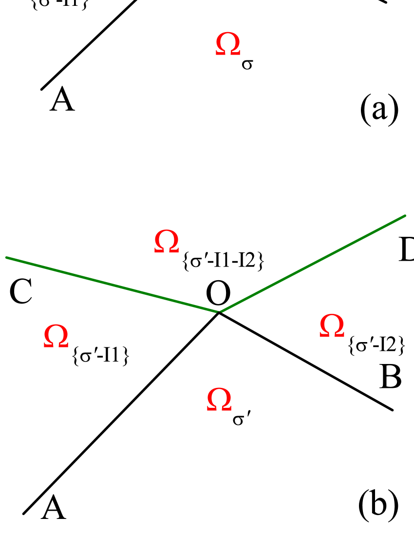
Figure 1: A draft to demonstrate the possible neighboring domains of $\Omega_{\sigma^{\prime}}$ plotted in the r-z plane.

(1) When two inherent segments of $\Omega_{\sigma^{\prime}}$ (specified by $\phi_{I_{1}}^{\sigma^{\prime}}=0$ and $\phi_{I_{2}}^{\sigma^{\prime}}=0$) intersect at a curve $C_{I_{1}I_{2}}$, we introduce a draft shown in Fig.1a, which is plotted in the X-Z plane while $y$ is fixed. Where, the two inherent segments are marked as $\overset{\_\_}{AOA^{\prime}}$ and $\overset{\_\_}{BOB^{\prime}}$, the curve $C_{I_{1}I_{2}}$ is marked as a point $O$, and the domain $\Omega_{\sigma^{\prime}}$ is bound by $\overset{\_\_}{AOB}$. The domain by the other side of $\overset{\_\_}{AO}$ is $\Omega_{\{\sigma^{\prime}-I_{1}\}}$. We assume that, for an index $I_{x}\in\{\sigma^{\prime}-I_{1}\}$, the inherent segment of $\Omega_{\{\sigma^{\prime}-I_{1}\}}$ specified by $\phi_{I_{x}}^{\{\sigma^{\prime}-I_{1}\}}=0$ intersects $\overset{\_\_}{AO}$ at $O^{\prime}$. Let this segment be marked by $\overset{\_\_}{O^{\prime}C}$ as shown in 1a, thus we have

$$\phi_{I_{x}}^{\{\sigma^{\prime}-I_{1}\}}|_{\overset{\_\_}{O^{\prime}C}}=0$$ (18)

On the other hand, recall that $\overset{\_\_}{AO}$ is an inherent segment of $\Omega_{\sigma^{\prime}}$ at which $\phi_{I_{1}}^{\sigma^{\prime}}=0$ but $\phi_{I_{x}}^{\sigma^{\prime}}\neq 0$. Thus we have

$$\phi_{I_{x}}^{\sigma^{\prime}}|_{\overset{\_\_}{AO}}\neq 0$$ (19)

Since $O^{\prime}$ is a point at $\overset{\_\_}{O^{\prime}C}$ and also at $\overset{\_\_}{AO}$, from eqs.(18,19) we have

$\phi_{I_{x}}^{\{\sigma^{\prime}-I_{1}\}}|_{O^{\prime}}\neq\phi_{I_{x}}^{\sigma^{\prime}}|_{O^{\prime}}$. This is in contradiction with the Feature I unless $I_{x}=I_{2}$ and $O^{\prime}=O$ (in this case the inequality eq.(19) becomes an equality at $O$). In fact, the inherent segment (specified by $\phi_{I_{2}}^{\{\sigma^{\prime}-I_{1}\}}=0$) must intersect $\overset{\_\_}{AO}$ at $O$, because $O$ is the only point at $\overset{\_\_}{AO}$ where $\phi_{I_{2}}^{\{\sigma^{\prime}-I_{1}\}}$ could be zero. Thus, we have proved that the part of boundary of $\Omega_{\{\sigma^{\prime}-I_{1}\}}$ will be connected as $\overset{\_\_}{AOC}$ as shown in Fig.1b. Obviously, the domain by the other side of $\overset{\_\_}{OC}$ is $\Omega_{\{\sigma^{\prime}-I_{1}-I_{2}\}}$.

Incidentally, if one can tune the parameters so that the segment $\phi_{J}^{\{\sigma^{\prime}-I_{1}+J\}}=0$ ($J\notin\sigma^{\prime}$) can intersect $\overset{\_\_}{AO}$ exactly at $O$, this segment may be optionally introduced as an embedded segment to replace the inherent segment $\overset{\_\_}{OC}$. But this phenomenon is very improbable to occur (i.e., it occurs only if the parameters are given at a particular point in the parameter-space).

With a similar argument we can deduce that the other neighbor of $\Omega_{\sigma^{\prime}}$ is $\Omega_{\{\sigma^{\prime}-I_{2}\}}$, and the inherent segment of $\Omega_{\{\sigma^{\prime}-I_{2}\}}$ that connects $O$ is the one specified by $\phi_{I_{1}}^{\{\sigma^{\prime}-I_{2}\}}=0$ (marked by $\overset{\_\_}{OD}$ as shown in 1b). The domain bounded by $\overset{\_\_}{COD}$ should be $\Omega_{\{\sigma^{\prime}-I_{1}-I_{2}\}}$. Thus, the neighborhood of $C_{I_{1}I_{2}}$ is characterized by having four surfaces converging at $C_{I_{1}I_{2}}$. During the extension by crossing over $\overset{\_\_}{OA}$ and $\overset{\_\_}{OC}$ (or $\overset{\_\_}{OB}$ and $\overset{\_\_}{OD}$), the species number $K^{\prime}$ decreases by two.

(2) When an embedded segment of $\Omega_{\sigma^{\prime}}$ (specified by $\phi_{J_{1}}^{\{\sigma^{\prime}+J_{1}\}}=0$ and marked by $\overset{\_\_}{AO}$ in Fig.1c) and another embedded segment (by $\phi_{J_{2}}^{\{\sigma^{\prime}+J_{2}\}}=0$ and by $\overset{\_\_}{BO}$) intersect at a curve $C_{J_{1}J_{2}}$ (marked by $O$), the neighboring domains will be $\Omega_{\{\sigma^{\prime}+J_{1}\}}$ and $\Omega_{\{\sigma^{\prime}+J_{2}\}}$, respectively. Let us first consider the boundary of $\Omega_{\{\sigma^{\prime}+J_{1}\}}$. We assume that an inherent segment specified by $\phi_{I}^{\{\sigma^{\prime}+J_{1}\}}=0$ ($I\in\sigma^{\prime}$) intersects $\overset{\_\_}{AO}$ at $O^{\prime}$. Note that $\phi_{I}^{\{\sigma^{\prime}+J_{1}\}}|_{\overset{\_\_}{AO}}=\phi_{I}^{\sigma^{\prime}}|_{\overset{\_\_}{AO}}$ (due to Feature I) while the latter $\phi_{I}^{\sigma^{\prime}}|_{\overset{\_\_}{AO}}\neq 0$ (because $\overset{\_\_}{AO}$ is embedded in the interior of $\Theta_{\sigma^{\prime}}$). Therefore, $O^{\prime}$ can not lie at $\overset{\_\_}{AO}$. It implies that any inherent segments of $\Omega_{\{\sigma^{\prime}+J_{1}\}}$ can not touch $\overset{\_\_}{AO}$, and therefore the part of boundary extending from $\overset{\_\_}{AO}$ can only be an embedded segment.

We assume that an embedded segment $\phi_{J_{2}}^{\{\sigma^{\prime}+J_{1}+J_{2}\}}=0$ intersects $\overset{\_\_}{AO}$ at $O"$ as shown in 1c. Then we have

$$\phi_{J_{2}}^{\{\sigma^{\prime}+J_{1}+J_{2}\}}|_{O"}=0.$$ (20)

Recall that the other segment of $\Omega_{\sigma^{\prime}}$ is marked by $\overset{\_\_}{BO}$ at which $\phi_{J_{2}}^{\{\sigma^{\prime}+J_{2}\}}=0$. Since $O"$ is lower than $O$ as shown in 1c, we have

$$\phi_{J_{2}}^{\{\sigma^{\prime}+J_{2}\}}|_{O"}<0$$ (21)

However, due to the continuity of the wave function of the $J_{1}-$species at $\overset{\_\_}{O"C}$, we have

$\phi_{J_{1}}^{\{\sigma^{\prime}+J_{1}+J_{2}\}}|_{\overset{\_\_}{O"C}}=\phi_{J_{1}}^{\{\sigma^{\prime}+J_{1}\}}|_{\overset{\_\_}{O"C}}$. When the coordinates tend to $O"$, the latter tends to zero. Thus we have $\phi_{J_{1}}^{\{\sigma^{\prime}+J_{1}+J_{2}\}}|_{O"}=0$. Since the wave function of the $J_{1}-$species is zero at $O"$, the two sets $\{\phi^{\{\sigma^{\prime}+J_{1}+J_{2}\}}\}$ and $\{\phi^{\{\sigma^{\prime}+J_{2}\}}\}$ should be one-by-one equal at $O"$ (due to Feature I). In particular, we have

$$\phi_{J_{2}}^{\{\sigma^{\prime}+J_{1}+J_{2}\}}|_{O"}=\phi_{J_{2}}^{\{\sigma^{\prime}+J_{2}\}}|_{O"}.$$ (22)

The above three equations eqs.(20,21,22) lead to a contradiction, unless $O"$ and $O$ overlap. Thus we have proved that the extension of $\overset{\_\_}{AO}$ is the embedded segment $\overset{\_\_}{OC}$ (specified by $\phi_{J_{2}}^{\{\sigma^{\prime}+J_{1}+J_{2}\}}=0$), and the part of boundary of $\Omega_{\{\sigma^{\prime}+J_{1}\}}$ is $\overset{\_\_}{AOC}$ as shown in 1c. During the crossing over $\overset{\_\_}{AO}$ and $\overset{\_\_}{OC}$, $\Omega_{\sigma^{\prime}}\rightarrow\Omega_{\{\sigma^{\prime}+J_{1}\}}\rightarrow\Omega_{\{\sigma^{\prime}+J_{1}+J_{2}\}}$. As before, one can tune the parameters so that the segment $\phi_{J_{3}}^{\{\sigma^{\prime}+J_{1}+J_{3}\}}=0$ ($J_{3}\neq J_{2}$) intersects $\overset{\_\_}{AO}$ also at $O$. This phenomenon is omitted due to the very small probability (i.e., the parameters are given at a particular set of values).

With a similar argument, for $\Omega_{\{\sigma^{\prime}+J_{2}\}}$, the extension of $\overset{\_\_}{BO}$ is also an embedded segment specified by $\phi_{J_{1}}^{\{\sigma^{\prime}+J_{1}+J_{2}\}}=0$ (marked by $\overset{\_\_}{OD}$). The domain by the other side of $\overset{\_\_}{OD}$ is also $\Omega_{\{\sigma^{\prime}+J_{1}+J_{2}\}}$. The domains in the neighborhood of the intersection $C_{J_{1}J_{2}}$ is shown in Fig.1c. Note that, by defining $\sigma"=\sigma^{\prime}+J_{1}+J_{2}$, 1c becomes 1b with $\sigma^{\prime}$ being replaced by $\sigma"$. Similarly, by defining $\sigma^{\prime\prime\prime}=\sigma^{\prime}-I_{1}$, 1b can be re-plotted as 1d where an inherent segment and an embedded segment of $\Omega_{\sigma^{\prime}}$ intersect.

Fig.1 demonstrates qualitatively how the formal solutions will link up together so that the entire solution can extends outward from a specific domain $\Omega_{\sigma^{\prime}}$. Recall that there are options in the extension to be decided in advance. When the boundary of $\Omega_{\sigma^{\prime}}$ contains only a single inherent segment $\phi_{I_{o}}^{\sigma^{\prime}}=0$, the outer domain is just $\Omega_{\{\sigma^{\prime}-I_{o}\}}$, and $\Omega_{\sigma^{\prime}}$ as a whole is embraced by $\Omega_{\{\sigma^{\prime}-I_{o}\}}$.

VI An approach to obtain an entire solution

Based on the linking of the formal solutions, we propose the following approach to obtain the entire solutions for the CGP. Firstly we prescribe the form of the inmost domain where the origin is included. Due to the symmetry of the trap, we can consider only the first octant (i.e., $l\geq 0$). Secondly, when all the parameters $\gamma_{Il}$ and $\alpha_{IJ}$ are given, we presume all the values of $\varepsilon_{I}$. Then, all the coefficients involved in the formal solutions can be known. Thirdly, it is reminded that, during the extension from the inmost domain outward, we have the options to adopt embedded segments. It implies that we have the options to choose the neighbors with the choices shown in Fig.1. Where, when two domains are connected via a surface, the species numbers of the two differ by one. Whereas when two domains are connected only via a curve (say, $\Omega_{\sigma^{\prime}}$ and $\Omega_{\{\sigma^{\prime}-I_{1}-I_{2}\}}$ in Fig.1b), the species numbers differ by two. Nevertheless, we have to make all the options in advance. In this way we have prescribed (designed) a specific way to link up the formal solutions continuously to form a candidate of the entire solution. Of course, every kind of species must be included in the design. Note that, for an inherent segment of a domain with Form 1, the outer side of the segment is empty. According to Feature II no wave functions can emerge from an empty domain. Thus this inherent segment is the boundary of the whole condensate and the extension ends.

With a well defined design it turns out that the inputs (the parameters and the set $\{\varepsilon_{I}\}$) are seriously limited. For an example, if the inmost domain has been prescribed to have the Form $\sigma^{\prime}$, then all the $K^{\prime}$ coefficients $X_{I^{\prime}}^{\sigma^{\prime}}$ are required to be $>0$. Accordingly, constraints are imposed via the $K^{\prime}$ inequalities. In general, for each reasonable design, the inputs are constrained by a number of inequalities so that the parameters together with $\{\varepsilon_{I}\}$ are limited within a non-null specific scope (examples are given below). The last step is to introduce the $K$ equations of normalization. For a given set of parameters inside the scope, these equations are sufficient to determine the $K$ presumed values of $\{\varepsilon_{I}\}$. If the $\{\varepsilon_{I}\}$ so determined turn out to lie also inside the scope, then a realistic entire solution is thereby obtained (i.e., all the normalized wave functions together with $\{\varepsilon_{I}\}$ are known, and all the constraints are fulfilled). Otherwise or the scope itself is null, the design is unreasonable and should be revised. Examples with $K=4$ is given in the next section.

VII Examples with K=4

To demonstrate the realization of the above approach, two examples with $K=4$ are given below. For convenience, we assume that the trap is axial-symmetric with respect to the Z-axis, and we introduce $r^{2}=x^{2}+y^{2}$. As mentioned, the values of $\{\gamma_{Il}\}$, $\{\alpha_{IJ}\}$, and $\{\varepsilon_{I}\}$ have been presumed so that all formal solutions are well defined.

(1) Example 1.

Let the four kinds of atoms are denoted by I, II, III, and IV. Let $\sigma_{4}$ denote the set containing I to IV, $\sigma_{3}$ denote the set containing I to III, $\sigma_{2}$ denote the set containing I and II, while $\sigma_{1}$ denote the set containing I only. The design for a miscible state is shown in Fig.2 where the domains for the formal solutions are plotted in the first quadrant of the $r-z$ plane.

For this miscible state analytical solution can be obtained (refer to jpa for $K=3$). However, analytical expressions for $K=4$ are very complicated and will not be given here. Instead, we will list all the inequalities for constraining the parameters, and we will present the numerical result with respect to a given set of parameters.

According to the design, the inmost domain (denoted as $\Omega_{\sigma_{4}}$) contain four kinds of atoms. Therefore it is required

(i) $X_{J}^{\sigma_{4}}>0$, $J=I$ to $IV$.

(ii) The outer boundary of $\Omega_{\sigma_{4}}$ is denoted by $S_{4}$, which is an inherent segment specified by $\phi_{IV}^{\sigma_{4}}|_{S_{4}}=X_{IV}^{\sigma_{4}}-Y_{IV,x}^{\sigma_{4}}r^{2}-Y_{IV,z}^{\sigma_{4}}z^{2}=0$. At $S_{4}$, $\phi_{I}^{\sigma_{4}}|_{S_{4}}>0$, $\phi_{II}^{\sigma_{4}}|_{S_{4}}>0$, and $\phi_{III}^{\sigma_{4}}|_{S_{4}}>0$ are required.

(iii) The outer boundary of $\Omega_{\sigma_{3}}$ is denoted by $S_{3}$ specified by $\phi_{III}^{\sigma_{3}}|_{S_{3}}=X_{III}^{\sigma_{3}}-Y_{III,x}^{\sigma_{3}}r^{2}-Y_{III,z}^{\sigma_{3}}z^{2}=0$. At this surface $\phi_{I}^{\sigma_{3}}|_{S_{3}}>0$ and $\phi_{II}^{\sigma_{3}}|_{S_{3}}>0$ are required

(iv) The outer boundary of $\Omega_{\sigma_{2}}$ is denoted by $S_{2}$ specified by $\phi_{II}^{\sigma_{2}}|_{S_{2}}=X_{II}^{\sigma_{2}}-Y_{II,x}^{\sigma_{2}}r^{2}-Y_{II,z}^{\sigma_{2}}z^{2}=0$. At this surface $\phi_{I}^{\sigma_{2}}|_{S_{2}}>0$ is required

(v) The outer boundary of $\Omega_{\sigma_{1}}$ is denoted by $S_{1}$ specified by $2\varepsilon_{1}-\gamma_{I,x}r^{2}-\gamma_{I,z}z^{2}=0$. $S_{1}$ is also the boundary of the whole system.

(vi) Furthermore, since $S_{4}$, $S_{3}$, and $S_{2}$ are assumed to be an ellipsoid, it is required

$Y_{IV,x}^{\sigma_{4}}>0$ and $Y_{IV,z}^{\sigma_{4}}>0$; $Y_{III,x}^{\sigma_{3}}>0$ and $Y_{III,z}^{\sigma_{3}}>0$; and $Y_{II,x}^{\sigma_{2}}>0$ and $Y_{II,z}^{\sigma_{2}}>0$.

(vii) Finally, the four equations of normalization

$1=\int\phi_{J}^{2}d\Omega$

are required, where $\phi_{J}=\phi_{J}^{\sigma_{L}}$ if $d\Omega$ is in $\Omega_{\sigma_{L}}$, $J$ and $L$ are from $I$ to $IV$.

The parameters are given as: $N_{I}=55000$, $N_{II}=37500$, $N_{III}=25000$, $N_{IV}=12500$. The intra-species interactions in the unit $\hbar\omega\lambda^{3}$ are $c_{I}=c_{II}=c_{III}=c_{IV}=10^{-3}$. All the inter-species interactions in $\hbar\omega\lambda^{3}$ are $c_{JJ^{\prime}}=3\times 10^{-4}$. $\gamma_{Jx}=\gamma_{Jy}=1$ and $\gamma_{Jz}=1.5$ (where $J=I$ to $IV$). Then, the corresponding solution of the CGP has the chemical potentials (in $\hbar\omega$) $\varepsilon_{I}=4.56$, $\varepsilon_{II}=4.25$, $\varepsilon_{III}=3.98$, $\varepsilon_{IV}=3.64$. Fig.2 demonstrates not only the design but also the exact locations of the domains. The wave functions $\phi_{J}$ ($J=$I to IV) are shown in Fig.3.

Figure 2: The distribution of the species in Example 1. The space are divided into domains each supports a type of formal solution (plotted in the upper r-z plane). The labels of the domains are marked. The unit for distance is $\lambda\equiv\sqrt{\hbar/(m\omega)}$ (the same in the following figures).

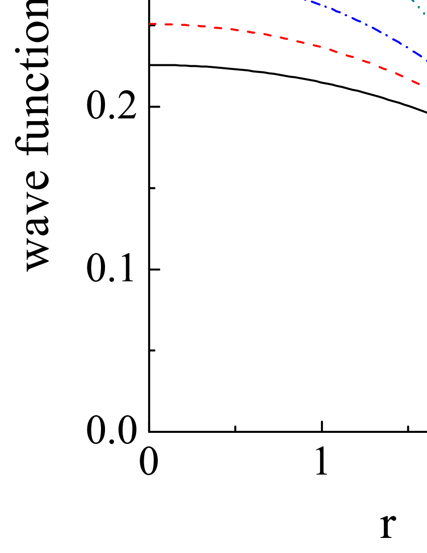
Figure 3: The wave functions in Example 1 plotted versus $r$ when $z=0$ (a), and versus $z$ when $r=0$ (b). $\phi_{I},\phi_{II},\phi_{III}$, and $\phi_{IV}$ are given in solid, dashed, dash-dot, and dash-dot-dot lines, respectively

(2) Example 2.

The design is shown in Fig.4. There are two intersecting inherent segments (as in Fig.1b), denoted as $S_{4}$ (the upper boundary of $\Omega_{\sigma_{4}}$) and $S_{4}^{\prime}$ (the right boundary of $\Omega_{\sigma_{4}}$), contained in the inmost domain. In addition to $\sigma_{3}$, the set $\sigma_{3}^{\prime}$ is introduced which contains I, II, and IV. The corresponding domains are $\Omega_{\sigma_{3}}$ and $\Omega_{\sigma_{3}^{\prime}}$, their right boundaries are denoted as $S_{3}$ and $S_{3}^{\prime}$, respectively

The constraints imposing upon the parameters and $\{\varepsilon_{I}\}$ are as follows

(i) The four inequalities $X_{J}^{\sigma_{4}}>0$ hold as in Example 1.

(iia) At the segment $S_{4}$, $\phi_{I}^{\sigma_{4}}|_{S_{4}}>0$, $\phi_{II}^{\sigma_{4}}|_{S_{4}}>0$, $\phi_{III}^{\sigma_{4}}|_{S_{4}}>0$, and $\phi_{IV}^{\sigma_{4}}|_{S_{4}}=0$.

(iib) At the segment $S_{4}^{\prime}$, $\phi_{I}^{\sigma_{4}}|_{S_{4}^{\prime}}>0$, $\phi_{II}^{\sigma_{4}}|_{S_{4}^{\prime}}>0$, $\phi_{IV}^{\sigma_{4}}|_{S_{4}^{\prime}}>0$, and $\phi_{III}^{\sigma_{4}}|_{S_{4}^{\prime}}=0$.

(iiia) At the segment $S_{3}$, $\phi_{I}^{\sigma_{3}}|_{S_{3}}>0$, $\phi_{II}^{\sigma_{3}}|_{S_{3}}>0$, and $\phi_{III}^{\sigma_{3}}|_{S_{3}}=0$.

(iiib) At the segment $S_{3}^{\prime}$, $\phi_{I}^{\sigma_{3}^{\prime}}|_{S_{3}^{\prime}}>0$, $\phi_{II}^{\sigma_{3}^{\prime}}|_{S_{3}^{\prime}}>0$, and $\phi_{IV}^{\sigma_{3}^{\prime}}|_{S_{3}^{\prime}}=0$ .

Furthermore, the points (iv), (v), (vi), and (vii) of Example 1 hold also in Example 2. In addition, $Y_{III,x}^{\sigma_{4}}>0$, $Y_{III,z}^{\sigma_{4}}>0$, $Y_{IV,x}^{\sigma_{3}^{\prime}}>0$ and $Y_{IV,z}^{\sigma_{3}^{\prime}}>0$ are required.

The parameters are adopted as:

$N_{I}=62500$, $N_{II}=45000$, $N_{III}=25000$, $N_{IV}=25000$. $\gamma_{Ix}=\gamma_{IIx}=0.8$, $\gamma_{Iz}=\gamma_{IIz}=0.7$,$\ \gamma_{IIIx}=1.2$ and $\gamma_{IIIz}=0.8$, while $\gamma_{IVx}=0.8$ and $\gamma_{IVz}=1.2$. For the interactions, $c_{I}=c_{II}=c_{III}=c_{IV}=10^{-3}$ and $c_{JJ^{\prime}}=3\times 10^{-4}$ as in Example 1. Note that the III-atoms (IV-atoms) are prescribed to be looser (tighter) bound along z-axis, thus they can be distributed more extensive (compact) along z-axis. Then, the corresponding solution of the CGP has $\varepsilon_{I}=4.00$, $\varepsilon_{II}=3.78$, $\varepsilon_{III}=4.04$, $\varepsilon_{IV}=3.75$. In Fig.4, not only the design but also the exact locations of the domains are demonstrated. The wave functions $\phi_{J}$ ($J=$I to IV) are shown in Fig.5.

Figure 4: The same as Fig.2 but for Example 2.

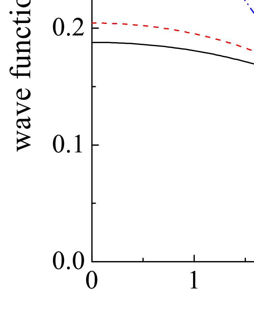
Figure 5: The same as Fig.3 but for Example 2.

VIII  Common features of $K-$species condensates and the inherent state-transition

We have proposed an approach to solve the CGP of the $K-$species condensates under the TFA. The traps for all the atoms have a common center. The common features of these systems are as follows:

(i) The entire solution is composed of the formal solutions, each hold in a specific domain and each contains specific kinds of atoms.

(ii) The domain that supports a specific formal solution can not extend along a direction infinitively (Feature II). Therefore, form-transformation is inevitable and the formal solutions are thereby linked up. During the linking of the formal solutions the wave function of every species remains continuous (Feature I).

(iii) No wave functions can emerge from an empty domain (due to Feature II). Thus the atoms can not be distributed in disconnected regions. Furthermore, the center of the traps can not be empty. In particular, the inherent segment of a domain with Form 1 is the outmost boundary of the whole system. This is because the domain next to the segment is empty.

(iv) Usually, the species numbers of two neighboring domains differ by one. However, for $K\geq 3$, the condensate may contain a special structure in which four domains with the Form $\sigma^{\prime}$, $\{\sigma^{\prime}-I_{1}\}$, $\{\sigma^{\prime}-I_{2}\}$, and $\{\sigma^{\prime}-I_{1}-I_{2}\}$, respectively, are neighboring to each other, and their boundaries converge at a curve at which $\phi_{I_{1}}=0$ and $\phi_{I_{2}}=0$. The convergence is shown in Fig.1 (where the set $\{\sigma^{\prime}-I_{1}-I_{2}\}$ might be null). It arises because the four sets of wave functions in the above four forms, respectively, will satisfy the same matrix-equation at the curve. Thus they are one-to-one equal at the curve, and therefore they converge. The convergence will be a popular phenomenon (but not of necessity) in K-species BEC.

(v) There are critical phenomena inherent in the multi-species BEC. When the strengths of interaction are tuned so that the matrix $[\alpha_{IJ}]$ tends to be singular (i.e., its determinant $D\rightarrow 0$), the wave functions in Form K will become extremely steep because $Y_{I,l}\rightarrow\pm\infty$ (refer to eq.(6,8)). When an entire solution of the CGP contains a Form K, during the crossing over the singular point of $[\alpha_{IJ}]$, $Y_{I,l}$ (for all $I$ and $l$) suddenly changes its sign and jumps from $+\infty$ to $-\infty$, or vice versa. Accordingly, the whole set of steeply down-falling wave functions suddenly become uprising, or vice versa. This causes a great change in the composition of the state, i.e., a state-transition. Accompanying the transition, the total energy increases remarkably as shown in the references jpb ; sr . Since all the K species are involved in this transition, it is called a full-state-transition. Obviously, the coupling among all the species contributes to this critical phenomenon. Therefore, when more and more species take part in the coupling, the critical point (i.e., the singular point of the matrix) will shift. The shift has been confirmed in a previous paper on 3- species BEC sr .

Furthermore, when an entire solution contains a Form $\sigma^{\prime}$ with $K^{\prime}$ species, the singular point of the $K^{\prime}-$rank matrix $[\alpha_{I^{\prime}J^{\prime}}]$ is also a critical point (where $D_{\sigma^{\prime}}=0$). The crossing over this point will lead also to a state-transition. However, during the transition, only the nonzero wave functions of the $K^{\prime}-$species are essentially involved (refer to eqs.(LABEL:fip,fils)), while the other are only slightly influenced (refer to sr ). Therefore, it is called a partial-state-transition. In this case, the transition is strongly affected by the interactions among the $K^{\prime}$ species but only weakly affected by the inter-species interaction imposed by the other $K-K^{\prime}$ species. In particular, the critical point of the partial-state-transition of the $K$-BEC is exactly the same as the full-state-transition of the $K^{\prime}$-BEC. When an entire solution contains a Form $\sigma^{\prime}$, the associated partial-state-transition might occur.

Note that the equation $D_{\sigma^{\prime}}=0$ specifies a surface in the parameter-space $\Sigma_{P}$. Therefore, each of the above critical point is in fact a critical surface in $\Sigma_{P}$. Thus, $\Sigma_{P}$ is divided into zones by a number of surfaces, one is related to the full-state-transition while the others are related to partial-state-transition. Each zone supports a specific phase. These zones might be further divided to give a more detailed classification on the composition. The division of $\Sigma_{P}$ into zones would lead to the phase-diagram.

Similar to the importance of the inter-species coupling in multi-species BEC, the inter-band coupling in multi-band superconductivity are found to be also important to the critical phenomena sup1 ; sup2 ; sup3 ; sup4 . Due to the coupling the critical points are therefore shifted. Moreover, the occurrence of the partial-state-transition can be regarded as a kind of hidden criticality, namely, the criticality of a sub-system (with a specific critical point) is hidden in the whole system and would emerge under certain conditions. This is more or less similar to the hidden criticality found in multi-band superconductivity sup2 .

Recall that, in the earliest study of the 2-species BEC, it has already been pointed out that the singular point of the two-rank matrix of the CGP induces instability ho96 . Obviously, the singularity of the matrix is an inherent feature of the CGP irrelevant to the TFA (refer to the last section of the ref. sr ). Therefore, the above state-transition is not a by-product of the TFA but an inherent physical phenomenon common to all $K-$BEC.

- (1) Myatt,C.J.,Burt,E.A.,Ghrist,R.W.,Cornell,E.A. and Wieman,C.E. Production of two overlapping Bose-Einstein condensate by sympathetic cooling, Phys. Rev. Lett. 78, 586-589 (1997).
- (2) Anderlini,M. et al. Sympathetic cooling and collisional properties of a Rb-Cs mixture, Phys. Rev. A 71 ,061401(R) (2005).
- (3) Ni,K.-K., et al. A high phase-space-density gas of polar molecules, Science 322, 231-235 (2008).
- (4) Pilch,K. et al. Observation of interspecies Feshbach resonances in an ultracold Rb-Cs mixture Phys. Rev. A 79, 042718 (2009)
- (5) Nemitz,N.,Baumer,F.,Münchow,F.,Tassy,S. and Görlitz,A. Production of heteronuclear molecules in an electronically excited state by photoassociation in a mixture of ultracold Yb and Rb, Phys. Rev. A 79, 061403 (2009) .
- (6) Wacker,L., et al. Tunable dual-species Bose-Einstein condensates of 39K and 87Rb, Phys. Rev. A 92, 053602 (2015).
- (7) Groebner,M., et al., A new quantum gas apparatus for ultracold mixtures of K and Cs and KCs ground-state molecules J. Modern Optics 63, 1829-1839 (2016)
- (8) Ho,T.L. and Shenoy,V.B. Binary mixtures of Bose condensates of alkali atoms. Phys. Rev. Lett. 77, 3276-3279 (1996).
- (9) Esry,B.D.,Greene,C.H.,Burke,J.P. and Bohn,J.L. Hartree-Fock theory for double condensates.Phys. Rev. Lett. 78, 3594-3597 (1997).
- (10) Pu,H. and Bigelow,N.P. Properties of two-species Bose condensates. Phys. Rev. Lett. 80, 1130-1133 (1998).
- (11) Chui,S.T. and Ao,P. Broken cylindrical symmetry in binary mixtures of Bose-Einstein condensates. Phys. Rev. A 59, 1473-1476 (1999).
- (12) Trippenbach,M.,Goral,K.,Rzazewski,K.,Malomed,B. and Band,Y. B. Structure of binary Bose-Einstein condebsates. J.Phys.B:At.Mol.Phys. 33, 4017-4031 (2000)
- (13) Riboli,F. and Modugno,M. Topology of the ground state of two interacting Bose-Einstein condensates. Phys. Rev. A 65, 063614 (2002).
- (14) Svidzinsky,A.A. and Chui,S.T. Symmetric-asymmetric transition in mixtures of Bose-Einstein condensates. Phys. Rev. A 67, 053608 (2003).
- (15) Luo,M.,Li,Z.B. and Bao,C.G. Bose-Einstein condensate of a mixture of two species of spin-1 atoms. Phys. Rev. A 75, 043609 (2007).
- (16) Luo,M.,Bao,C.G. and Li,Z.B. Spin evolution of a mixture of Rb and Na Bose–Einstein condensates: an exact approach under the single-mode approximation. Phys. B: At. Mol. Opt. Phys. 41, 245301(2008).
- (17) Galteland,P.N.,Babaev,E. and Sudbø,A. Thermal remixing of phase-separated states in two-component bosonic condensates. New J. Phys. 17, 103040 (2015).
- (18) VanSchaeybroeck,B. and Indekeu,J.O. Critical wetting, first order wetting, prewetting phase transitions in binary mixtures of Bose-Einstein condensates. Phys. Rev. A 91, 013626 (2015).
- (19) Indekeu,J.O.,Lin,C.Y.,Thu,N.V.Schaeybroeck,B.V., and Phat,T.H. Static interfacial properties of Bose-Einstein-condensate mixtures. Phys. Rev. A 91, 033615 (2015).
- (20) Kuopanportti,P., Orlova,T.V. and Milošević,M.V. Ground-state multiquantum vortices in rotating two-species superfluids, Phys. Rev. A 91, 043605 (2015).
- (21) Polo.J., et al., Analysis beyond the Thomas-Fermi approximation of the density profiles of a miscible two-component Bose-Einstein condensate. Phys. Rev. A 91, 053626 (2015).
- (22) You,J.S.,Liu,I.K. and Wang,D.W. Unconventional Bose-Einstein condensation in a system with two species of bosons in the p-orbital bands in an optical lattice. Phys. Rev. A 93, 053623 (2016).
- (23) Mujal,P.,Julia-Diaz,B. and Popps,A. Quantum properties of a binary bosonic mixture in a double well. Phys. Rev. A 93, 043619 (2016).
- (24) Cipolatti,R.,Villegas-Lelovsky,L.,Chung,M.C. and Trallero-Giner,C. Two-species Bose-Einstein condensates in an optical lattice: analytical approximate formulae. J.Phys. A 49, 145201 (2016).
- (25) Li,Z.B.,Liu,Y.M.,Yao,D.X., and Bao,C.G., Two types of phase-diaframs for two-species Bose-Einstein condensates and the combined effect of the parameters. J. Phys. B: At. Mol. Opt. Phys., 50 135301 (2017)
- (26) Liu,Y.M.,He,Y.Z.,Bao,C.G., Singularity in the matrix of the coupled Gross-Pitaevskii equations and the related state-transitions in three-species condensates. Scientific Reports, 7, 6585 (2017)
- (27) Suhl, H., Matthias, B. T. & Walker, L. R. Bardeen-Cooper-Schrieffer theory of superconductivity in the case of overlapping bands. Phys. Rev. Lett. 3, 552–554 (1959).
- (28) Komendova, L., Chen, Yajiang, Shanenko, A. A., Milosevic, M. V. & Peeters, F. M. Two-band superconductors: hidden criticality deep in the superconducting state. Phys. Rev. Lett. 108, 207002 (2012).
- (29) Stanev, V. & Tesanovic, Z. Three-band superconductivity and the order parameter that breaks time-reversal symmetry. Phys. Rev. B 81, 134522 (2010).
- (30) Silaev,M. & Babaev,E. Microscopic theory of type-1.5 superconductivity in multiband systems, Phys. Rev. B 84, 094515 (2011)
- (31) Caliari,M. and Squassina,M. Electronic Journal of Differential Equations, No.79 (2008)
- (32) Manikandan,K.,Muruganandam,P.,Senthilvelan,M., and Lakshmanan, M. Manipulating localized matter waves in multicomponent Bose-Einstein condensates. Phys. Rev. E 93, 032212 (2016)
- (33) Orlova,N.V.,Kuopanportti,P. and Milošević,M.V. Skyrmionic vortex lattices in coherently coupled three-component Bose-Einstein condensates. Phys. Rev. A 94, 023617 (2016).
- (34) Cipriani,M. and Nitta,M. Vortex lattices in three-component Bose-Einstein condensates under rotation: Simulating colorful vortex lattices in a color superconductor. Phys. Rev. A 88, 013634 (2013)
- (35) Liu,Y.M.,He,Y.Z.,Bao,C.G., Analytical solutions of the coupled Gross-Pitaevskii equations for three-species Bose-Einstein condensates. J. Phys. A: Math. Theor. 50 275301 (2017).
- (36) He,Y.Z.,Liu,Y.M. and Bao,C.G. Generalized Gross-Pitaevskii equation adapted to the U(5)-SO(5)-SO(3) symmetry for spin-2 condensates. Phys. Rev. A 91, 033620 (2015).