Compressive Time-of-Flight 3D Imaging Using Block-Structured Sensing Matrices

Abstract

Spatially and temporally highly resolved depth information enables numerous applications including human-machine interaction in gaming or safety functions in the automotive industry. In this paper, we address this issue using Time-of-flight (ToF) 3D cameras which are compact devices providing highly resolved depth information. Practical restrictions often require to reduce the amount of data to be read-out and transmitted. Using standard ToF cameras, this can only be achieved by lowering the spatial or temporal resolution. To overcome such a limitation, we propose a compressive ToF camera design using block-structured sensing matrices that allows to reduce the amount of data while keeping high spatial and temporal resolution. We propose the use of efficient reconstruction algorithms based on $\ell_{1}$-minimization and TV-regularization. The reconstruction methods are applied to data captured by a real ToF camera system and evaluated in terms of reconstruction quality and computational effort. For both, $\ell_{1}$-minimization and TV-regularization, we use a local as well as a global reconstruction strategy. For all considered instances, global TV-regularization turns out to clearly perform best in terms of evaluation metrics including the PSNR.

Keywords: Compressed sensing, Time-of-Flight Imaging, 3D Imaging, sparse recovery, total variation, image reconstruction.

1 Introduction

Time-of-Flight (ToF) camera systems rely on the time of flight (or travel time) of an emitted and reflected light beam to create a depth image of a scenery. They offer many advantages over traditional systems (e.g. lidar) such as compact design, registered depth and intensity images at a high frame rate, and low power consumption [14]. This makes them ideal for mobile usage, for example, on a mobile phone. On such devices, the computational resources for the required image reconstruction algorithms are limited. While there are several technologies allowing 3D imaging, in this paper we will focus on cameras that use a modulated light source to calculate the phase shift (encoding the depth image) between the emitted and received signal [18].

High spatial and temporal resolution requires a large amount of data to be read-out and transferred from ToF cameras. In order to determine a depth image, typically four different phase images per frame have to be collected with the ToF camera. However, even from four phase images, the depth image is unique only up to a certain maximal distance from the camera. To measure larger distances one needs additional phase images that have to be read-out and transferred. Also in multi-camera systems, where the depth image is calculated outside the camera, the amount of data can be very high. If the data rate or the read-out process is a limiting factor, either the spatial or the temporal resolution has to be reduced in a conventional ToF camera.

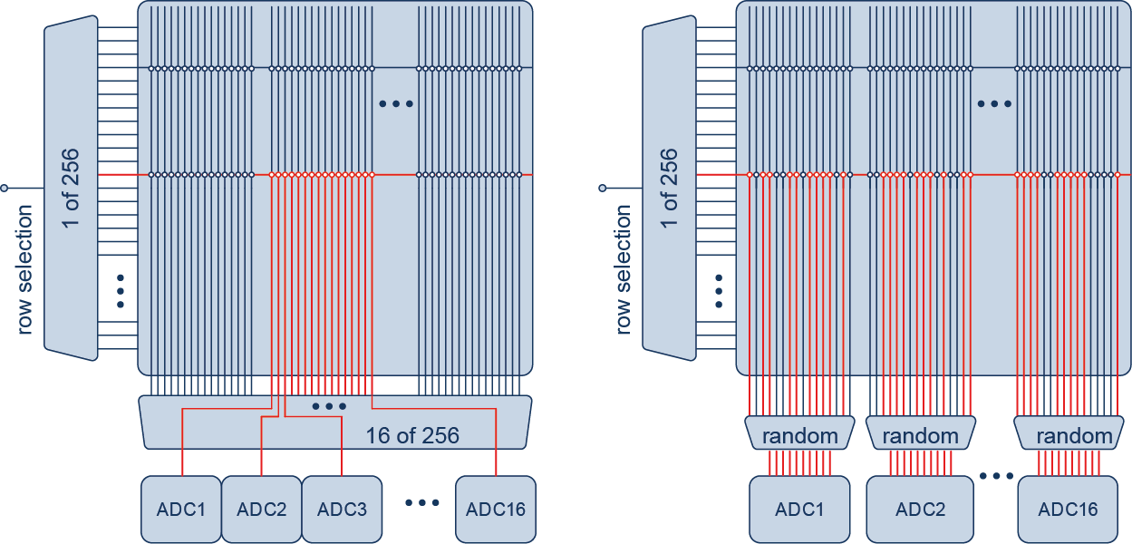
Figure 1.1: Standard read-out versus compressive read-out. Left: Standard sequential read-out using 16 ADCs used by our ToF camera. Right: Proposed compressive read-out. In each row, instead of 16 sequential read-outs per ADC, $m/K$ combinations of pixel values are read-out. Note that compared to the standard camera design, the main difference is the used multiplexer that combines the read-outs within a single block according the used measurement matrix.

Proposed compressive ToF imaging approach

To address the issues mentioned above, in this article we propose a compressive ToF camera that allows a reduced amount of data to be read-out and transferred while preserving high spatial and temporal resolution. Instead of individual pixels of the phase images, the compressive ToF camera reads out combinations of pixel values that are transferred to an external processor. As shown in Figure 1.1, the only additional element that has to be added to the existing camera design is multiplexer per block, which combines the pixels read-out according to the used measurement design. Note that multiplexers are standard element in CMOS (complementary metal-oxide-semiconductor) sensors [37]. Therefore, the proposed camera design only requires small modification of the existing camera design shown in Figure 1.1, left. As in the existing used ToF camera we only use combinations of elements in the same row which yields to block-structured sensing matrices. The actual manufacturing of such a compressive camera design is beyond the scope of this paper. Note that by using modern multi-layer circuit routing technology [23], one could also use combinations from different overlapping routing paths. We restrict our ourselves to the block-structured sensing matrices because they are compatible with the existing ToF camera design.

In order to reconstruct the original phase and depth images we use techniques from sparse recovery using $\ell_{1}$-minimization and total variation (TV)-regularization. For both methods we implemented a block based local approach as well as global approach. In all instances the global TV-regularization turns out tot outperform the other tested reconstruction methods in terms of RMAE (relative mean absolute error), PSNR (peak signal to noise ratio) as well as visual inspection. For example, using a compression ratio of 4.7, global TV-regularization yields a PSNR of 31.5 for the recovered depth image of a typical scenery, opposed to a PSNR of 26.4, 28.0 and 27.3 for block $\ell^{1}$-minimization, global $\ell^{1}$-minimization and block TV-regularization. We address this to the following issue. Depth images and phase will typically be piecewise homogeneous. Hence the depth images have sparse gradients which exactly is what TV-regularization tries to recover.

We point out that the proposed compressed sensing framework aims to accelerate the camera read-out and not to reduce the number of sensing pixels itself, which would be another interesting line of research. Different compressive ToF camera designs have been proposed in [24, 12, 22, 19]. The compressive designs in [24, 19] use a spatial light modulator and multiple pulses, whereas [22] uses coded aperture to gather multiple measurements. In [12], compressed sensing ToF imaging has been studied in the spatial and temporal domain. All these works use unstructured sensing matrices. In contrast to that, we use block-structured sensing matrices which are easier to implement in existing ToF camera designs. Additionally, the reduction of read-outs allows high spatial and temporal resolution.

Some results of this paper have been presented at the International Conference on Sampling Theory and Applications (SampTA) 2017 in Tallinn [3]. The present paper extends the theoretical recovery results stated in [3] from the standard basis to a general sparsifying basis. Additionally, all numerical studies presented in this paper are new and extended significantly compared to [3]. In particular, the TV-regularization studies for the proposed ToF compressed sensing scheme are completely new.

Outline

In Section 2 we give a short introduction the ToF imaging. In Section 3 we present the type of measurements that we propose for compressive ToF imaging. We thereby start with details on the classical (non-compressive) and the new (compressive) designs. Additionally, we prove that the used matrices fulfill the RIP under suitable conditions. Moreover, in Section 3 we also introduce the proposed block based image reconstruction approach using $\ell^{1}$-minimization and total variation. In the special cases of single blocks, we obtain the global counterparts. In Section 4 we give details on the numerical algorithm and present extensive studies of our two-step reconstruction approach of recovering the depth image from the compressed measurements. We compare the block-based as well as global version for $\ell^{1}$-minimization and TV-regularization. The results are evaluated in terms of RMAE and PSNR. Visually as well as in terms of these quality measures global TV-regularization outperforms the other methods in all instances.

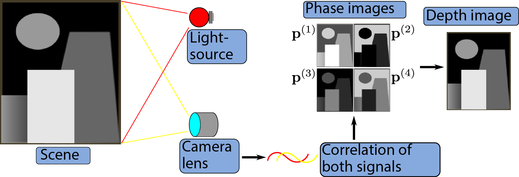
Figure 1.2: Basic principles of a ToF camera. Phase images are collected by sampling the cross-correlation of the emitted with the reflected light pulse. From these phase images one computes a depth image mapping the distance from the scene to the camera.

2 Basics of 3D imaging using ToF cameras

A ToF camera measures the distance of a scenery to the camera. By sending out a diffuse light pulse and measuring the reflected signal, the camera is able to record depth information of the entire scenery at once. To acquire depth information, the sent out light is modulated and can be generated by an LED. The scenery reflects the light which is recorded by the camera as depicted in Figure 1.2. The emitted pulse can be modeled as a time-dependent function $g(t)=C\cos(\omega t)$, where $C$ is the amplitude, $\omega$ the modulation frequency (or carrier frequency), and $t$ the time variable. The signal is reflected, and the camera receives, for any individual pixel $i\in\{1,\ldots,n\}$, a phase and amplitude shifted signal

$$f_{i}(t)=B_{i}+A_{i}\cos(\omega t-\varphi_{i})\,.$$

Here $\varphi_{i}$ is the phase shift depending on the distance $d_{i}$ between the camera and the scene mapped at pixel $i$, $A_{i}$ the amplitude depending on the reflectivity, and $B_{i}$ an offset. The phase shift is related to the distance $d_{i}$ via the relation $d_{i}=\varphi_{i}\;c/(2\omega)$.

At each pixel of the ToF camera, the cross-correlation between the reference and the reflected signal is measured, where the cross-correlation between two signals $f\colon\mathds{R}\to\mathds{R}$ and $g\colon\mathds{R}\to\mathds{R}$ is given by

$$c_{f,g}(s)=\lim_{T\to\infty}\frac{1}{2T}\int_{-T}^{T}\!{f(t)g(t+s)}\,\mathrm{d}{t}\,.$$ (2.1)

In our case, $c_{f,g}(\cdot)$ can be calculated analytically [1, 29, 18] which yields

$$c_{f_{i},g}(s)=\frac{A_{i}C}{2}\cos(\omega s+\varphi_{i})+K_{i}\,.$$ (2.2)

Here $K_{i}$ incorporates constants accounting for noise and the background image generated by ambient light. By sampling the cross-correlation function at the sampling points $s\in\{0,\pi/(2\omega),\pi/\omega,3\pi/(2\omega)\}$ we get four so-called phase images

$$\mathbf{p}^{(1)} =\phantom{-}\frac{\mathbf{A}C}{2}\cos(\boldsymbol{\varphi})+\mathbf{K}$$

$$\mathbf{p}^{(2)} =-\frac{\mathbf{A}C}{2}\sin(\boldsymbol{\varphi})+\mathbf{K}$$

$$\mathbf{p}^{(3)} =-\frac{\mathbf{A}C}{2}\cos(\boldsymbol{\varphi})+\mathbf{K}$$

$$\mathbf{p}^{(4)} =\phantom{-}\frac{\mathbf{A}C}{2}\sin(\boldsymbol{\varphi})+\mathbf{K}\,.$$

Here we have set $\boldsymbol{\varphi}\triangleq(\varphi_{j})_{j=1}^{n}\in\mathds{R}^{n}$, $\mathbf{K}\triangleq(K_{j})_{j=1}^{n}$ and $\mathbf{A}\triangleq(A_{j})_{j=1}^{n}\in\mathds{R}^{n}$, and all operations are taken point-wise. Under the common assumption that $K_{i}$ is independent of the pixel location we can estimate the phase shifts $\boldsymbol{\varphi}$ by

$$\hat{\boldsymbol{\varphi}}=\operatorname{\arg}\left(\mathbf{p}^{(1)}-\mathbf{p}^{(3)}+i\bigl{(}\mathbf{p}^{(4)}-\mathbf{p}^{(2)}\bigr{)}\right)\,.$$ (2.3)

Here $\alpha=\operatorname{\arg}(z)\in[0,2\pi)$ denotes the argument of the complex number $z$ defined by $z\triangleq re^{i\alpha}$. In particular, the depth image is given by $\hat{\mathbf{d}}=\hat{\boldsymbol{\varphi}}\;c/(2\omega)$.

Since the phase shifts are contained in $[0,2\pi)$, the maximal distance that can be found by (2.3) is $d_{\max}=(c/\omega)\pi$. Larger distances are falsely identified, taking values in the interval $[0,d_{\max})$. To overcome this ambiguity, several methods have been proposed in the literature (see, for example,  [18, 13]). One such approach consists in capturing two sets of phase images with different modulation frequencies $\omega_{1}\neq\omega_{2}$, and then comparing the two depth images. In this paper, we will not address the ambiguity problem further. The compressive ToF camera that we propose below can be extended to multiple modulation frequencies in a straightforward manner. Sparse recovery can be applied to any of the phase images, even if they are affected by phase wrapping. Further research, however, is needed to thoroughly investigate such extensions, in particular, to investigate sparsity issues, accuracy and noise stability.

3 Compressive ToF sensing and image reconstruction

In this section we present the proposed compressive ToF 3D sensing design compatible with existing ToF cameras. Additionally, we describe an efficient block-wise reconstruction procedure based on sparse recovery.

3.1 Compressive ToF sensing

As mentioned in the introduction, in a conventional ToF camera, all pixel values of all phase images have to be read-out and large amounts of data have to be transferred. To reduce the amount of data, in this paper, we propose a compressive ToF camera, which reads out and transmits linear combinations instead of individual pixel values of the phase image. Our proposed compressive ToF camera design is based on the existing non-compressive ToF camera design, which should allow to engineer and build the new camera with low effort. The only difference between the two designs is in the way the pixels of the sensors are read-out. For the compressive ToF camera, we propose to read-out linear combinations of neighboring pixels.

The data collected by the compressive ToF camera can be written in the form

$$\forall i\in\{1,2,3,4\}\colon\quad\mathbf{y}^{(i)}=\mathbf{M}\mathbf{p}^{(i)}\,.$$

Here $\mathbf{M}\in\mathds{R}^{m\times n}$ is the measurement matrix, $\mathbf{p}^{(i)}\in\mathds{R}^{n}$ are the phase images and $\mathbf{y}^{(i)}\in\mathds{R}^{m}$ the read-out data with $m\ll n$. To reconstruct the depth image from the compressed read-outs we propose the following two-step procedure: First, we estimate the differences $\mathbf{p}^{(1)}-\mathbf{p}^{(3)}$ and $\mathbf{p}^{(4)}-\mathbf{p}^{(2)}$ from

$$\mathbf{y}^{(1)}-\mathbf{y}^{(3)} =\mathbf{M}\left(\mathbf{p}^{(1)}-\mathbf{p}^{(3)}\right)\,,$$ (3.1)

$$\mathbf{y}^{(4)}-\mathbf{y}^{(2)} =\mathbf{M}\left(\mathbf{p}^{(4)}-\mathbf{p}^{(2)}\right)\,,$$ (3.2)

using sparse recovery. In a second step we recover the depth image by applying (2.3) to the estimated differences.

Any of the equations (3.1), (3.2) is an underdetermined system of the form $\mathbf{y}=\mathbf{M}\mathbf{x}$, for which in general no unique solution exists. To obtain solution uniqueness, the vector $\mathbf{x}\in\mathds{R}^{n}$ needs to satisfy certain additional requirements. In recent years, sparsity turned out to be a powerful property for this purpose. Recall that $\mathbf{x}$ is called $s$-sparse, if it has at most $s$ nonzero entries. Assuming sparsity, the vector $\mathbf{x}$ can, for example, be recovered by solving the $\ell_{1}$-minimization problem

$$\operatorname*{minimize}_{\mathbf{z}\in\mathds{R}^{n}}\lVert\mathbf{z}\rVert_{1}\quad\text{subject to }\mathbf{M}\mathbf{z}=\mathbf{y}\,.$$ (3.3)

In order for (3.3) to uniquely recover $\mathbf{x}$, the matrix $\mathbf{M}$ needs to fulfill certain properties. One sufficient condition is the restricted isometry property (RIP). The matrix $\mathbf{M}$ is said to satisfy the $s$-RIP with constant $\delta>0$, if

$$(1-\delta)\lVert\mathbf{z}\rVert_{2}^{2}\leq\lVert\mathbf{M}\mathbf{z}\rVert_{2}^{2}\leq(1+\delta)\lVert\mathbf{z}\rVert_{2}^{2}$$

holds for all $s$-sparse $\mathbf{z}\in\mathds{R}^{n}$. If the $s$-RIP constant is sufficiently small, then (3.3) uniquely recovers any sufficiently sparse vector (see, for example,  [10, 15, 7]).

Although some results for deterministic RIP matrices exist [20, 6], matrices satisfying the RIP are commonly constructed in some random manner. Realizations of Gaussian or Rademacher random matrices are known to satisfy the RIP with high probability [15]. Rademacher random variables take the values -1 and 1 with equal probability. It has been shown [8] that if $m\geq C\delta^{-2}s\log(n/s)$, then $\delta_{s}\leq\delta$ with high probability for both types of matrices. Note that up to the logarithmic factor, this bound scales linearly in the sparsity level $s$. In this sense, the bound is optimal in the sparsity level, because $m\geq 2s$ is the minimal requirement for any measurement matrix to be able to recover all $s$-sparse vectors [15]. More generally, all matrices with independent sub-Gaussian entries satisfy the RIP with high probability. A sub-Gaussian random variable $X$ is defined by the property

$$\mathds{P}(\lvert X\rvert\geq t)\leq\beta\mathrm{e}^{-\kappa t^{2}}\quad\text{for all }t>0$$ (3.4)

with constants $\beta,\kappa>0$. It is easy to show that Rademacher and Gaussian random variables are sub-Gaussian. Sub-Gaussian matrices $\mathbf{M}$ are also universal [15] which means that for any unitary matrix $\boldsymbol{\Psi}\in\mathds{C}^{n\times n}$ the matrix $\mathbf{M}\boldsymbol{\Psi}$ also satisfies the RIP. Thus one can also recover signals that are not sparse in the standard basis but for which $\boldsymbol{\Psi}^{\ast}\mathbf{x}$ is sparse, where $\boldsymbol{\Psi}^{\ast}$ is the conjugate transpose. This property is very useful in applications since many natural signals have sparse representations in certain bases different from the standard basis. In general, if the restricted isometry constant of $\mathbf{M}\boldsymbol{\Psi}$ is small, then we can recover the signal by solving (3.3) with $\mathbf{M}\boldsymbol{\Psi}$ instead of $\mathbf{M}$ and, in the noisy case, by

$$\operatorname*{minimize\,}_{\mathbf{z}\in\mathds{C}^{n}}\lVert\boldsymbol{\Psi}^{\ast}\mathbf{z}\rVert_{1}\quad\text{such that }\lVert\mathbf{M}\mathbf{z}-\mathbf{y}\rVert_{2}\leq\eta\,.$$ (3.5)

Here $\eta$ equals the noise level of the measurements. Similar results hold if $\boldsymbol{\Psi}$ is a frame (see [9, 17, 27, 34]).

In practical applications, such unstructured matrices cannot always be used. Either there are restrictions on the matrix preventing us from using a random matrix with i.i.d. entries or the storage space is limited, such that storing a full matrix would be too expensive. There are different methods for constructing structured compressed sensing matrices that satisfy the RIP. For example, such matrices can be constructed by random subsampling of an orthonormal matrix [15, Chapter 12] or deterministic convolution followed by random subsampling [30] or using a random convolution followed by deterministic subsampling [33]. In the next section we will examine the latter type since its application to ToF imaging and the existing camera designs they have beneficial properties. More specifically, such measurement matrices can be constructed to only use entries form a small set, such as $\{-1,0,1\}$, can efficiently be implemented by using Fourier transform techniques, and require litte information to be stored.

3.2 Compressive 3D Sensing Using Block Partial Circulant Matrices

The hardware requirements in our case prevent us from using arbitrary matrices since for the analog-to-digital converters (ADC) the weights 0 and $\pm a$ for some fixed constant $a\in\mathds{R}$ should be used. Further, any individual ADC can only be wired with a limited number of pixels (compare Figure 1.1) which imposes a particular block-structure of the measurement matrix. Thus, the measurement matrices that we use in our approach take the block-diagonal form

$$\mathbf{M}=\mathbf{M}_{1}\otimes\cdots\otimes\mathbf{M}_{K}\triangleq\begin{pmatrix}\mathbf{M}_{1}&\mathbf{0}&\cdots&\mathbf{0}\\ \mathbf{0}&\mathbf{M}_{2}&\cdots&\mathbf{0}\\ \vdots&&\ddots&\vdots\\ \mathbf{0}&\cdots&&\mathbf{M}_{K}\end{pmatrix}\,.$$ (3.6)

Here, each sub-matrix $\mathbf{M}_{k}\in\mathds{R}^{m_{k}\times n_{k}}$ operates on a certain subset $\Omega_{k}\subsetneq\{1,\ldots,n\}$ with $n_{k}=\lvert\Omega_{k}\rvert$ elements coming from a single row in the image. For simplicity we consider the case that $n_{k}=n/K$ and $m_{k}=m/K$ for each $k$. The particular measurements in each row block are constructed in a certain random manner satisfying the requirements above.

A particularly useful class of such row-wise measurements in the compressive ToF camera can be modeled by partial circulant matrices. A circulant matrix $\mathbf{C}_{\mathbf{v}}\in\mathds{R}^{n\times n}$ associated with $\mathbf{v}=(v_{1},\ldots,v_{n})\in\mathds{R}^{n}$ is defined by

$$\forall i,j\in\{1,\dots,n\}\colon\quad(\mathbf{C}_{\mathbf{v}})_{i,j}=v_{i\ominus j}\,,$$

where $j\ominus i\triangleq(j-i)\mod n$ is the cyclic subtraction. In particular, for all $\mathbf{v},\mathbf{w}\in\mathds{R}^{n}$, we have $\mathbf{C}_{\mathbf{v}}\mathbf{w}=\mathbf{v}\ast\mathbf{w}$, where $(\mathbf{v}\ast\mathbf{w})_{j}\triangleq\sum_{i=1}^{n}v_{j\ominus i}w_{i}$ is the circular convolution. For any subset $\Omega\subseteq\{1,\ldots,n\}$, the projection matrix $\mathbf{R}_{\Omega}\in\mathds{R}^{|\Omega|\times n}$ is defined by $\mathbf{R}_{\Omega}\mathbf{v}\triangleq(\mathbf{v}_{i})_{i\in\Omega}$.

Definition 3.1.

The partial circulant matrix associated to $\mathbf{v}\in\mathds{R}^{n}$ and $\Omega\subseteq\{1,\ldots,n\}$ is defined by $\frac{1}{\sqrt{\lvert\Omega\rvert}}\mathbf{R}_{\Omega}\mathbf{C}_{\mathbf{v}}$.

Further, recall that a random vector $\mathbf{v}$ with values in $\{\pm 1\}^{n}$ is called a Rademacher vector if it has independent entries taking the values $\pm 1$ with equal probability. Partial circulant matrices satisfy the RIP. Such results have been obtained first in [33] and have later been refined in [26, Theorem 1.1] using the theory of suprema of chaos processes. These results have been formulated for sparsity in the standard basis. For our purpose, we formulate such a result for the general orthonormal bases.

Theorem 3.2.

Consider the partial circulant matrix $\mathbf{M}=\frac{1}{\sqrt{m}}\mathbf{R}_{\Omega}\mathbf{C}_{\mathbf{v}}$ associated to a vector $\mathbf{v}$ with iid sub-Gaussian entries and a subset $\Omega\subseteq\{1,\ldots,n\}$ containing $m$ elements. If, for some $s\leq n$ and $\delta\in(0,1)$, we have

$$m\geq C\delta^{-2}\mu^{2}s(\log s)^{2}(\log n)^{2}\,,$$

then, with probability at least $1-n^{-\log n\log^{2}s}$, the $s$-RIP constant of $\mathbf{M}\boldsymbol{\Psi}$ is at most $\delta$, where the constant $\mu$ is given by $\mu=\max_{i,j}\lvert\langle\mathbf{F}_{j-},\boldsymbol{\Psi}_{i-}\rangle\rvert$. Here $\mathbf{F}$ is the discrete Fourier matrix and $\boldsymbol{\Psi}\in\mathds{C}^{n\times n}$ is any unitary matrix.

Proof.

For the case that $\boldsymbol{\Psi}$ is the identity matrix the result is derived in the original paper [26]. The generalization to arbitrary $\boldsymbol{\Psi}$ can be shown analogously to the original results. Such a proof is worked out in [2, 4]. ∎

Theorem 3.2 shows that random partial circulant matrices yield stable recovery of sparse vectors using (3.3). Recall that the proposed compressive ToF camera read-out uses block diagonal measurement matrices of the form (3.6). Taking each block as a random partial circulant matrix and applying Theorem 3.2 yields the following result.

Theorem 3.3.

Let $\mathbf{M}\in\mathds{R}^{m\times n}$ be of the form (3.6), where each block on the diagonal is a partial circulant matrix $\mathbf{M}_{k}=\frac{1}{\sqrt{m_{k}}}\mathbf{R}_{\Omega_{k}}\mathbf{C}_{\mathbf{v}_{k}}$ associated with independent Rademacher vectors $\mathbf{v}_{k}$ and subsets $\Omega_{k}\subseteq\{1,\ldots,n/K\}$ having $m_{k}=m/K$ elements that are selected independently and uniformly at random. If, for some $s\in\mathds{N}$ and $\delta\in(0,1)$, we have

$$m\geq KC\delta^{-2}\mu^{2}s(\log s)^{2}(\log(n/K))^{2}\,,$$

then, with probability at least $(1-(n/K)^{-\log(n/K)\log^{2}s})^{K}$, $\mathbf{M}_{k}\boldsymbol{\Psi}$ has the $s$-RIP constant of at most $\delta$ for all $k=1,\ldots,K$. Here the constant $\mu$ is given by $\mu=\max_{i,j}\lvert\langle\mathbf{F}_{j-},\boldsymbol{\Psi}_{i-}\rangle\rvert$ and $\boldsymbol{\Psi}\in\mathds{C}^{(n/K)\times(n/K)}$ is any unitary matrix.

Proof.

As $m/K\geq C\delta^{-2}s(\log s)^{2}(\log(n/K))^{2}$, we can apply Theorem 3.2 with $n$ and $m$ replaced by $n/K$ and $m/K$ to each block. Thus the restricted isometry constant of each block is at most $\delta$ with probability at least $1-(n/K)^{-\log(n/K)\log^{2}s}$. As the generating Rademacher vectors for each block are independent, the $s$-RIP constants of all blocks are uniformly bounded by $\delta$ with probability at least $(1-(n/K)^{-\log(n/K)\log^{2}s})^{K}$. ∎

Theorem 3.3 yields stable recovery via (3.5) if the vector $\mathbf{x}$ is $\boldsymbol{\Psi}$-block sparse, meaning that $\mathbf{x}=\left[\mathbf{x}_{1},\ldots,\mathbf{x}_{K}\right]$ with $\boldsymbol{\Psi}^{\ast}\mathbf{x}_{k}\in\mathds{R}^{n/K}$ being $s$ sparse for all $k=1,\ldots,K$.

Note that a different compressive CMOS sensor design using partial circulant matrices has been proposed in [21]. Our design uses multiple ADCs (actually, the existing camera design suggests 16 ADCs) each of them operates on a small number of pixels. Thus our design uses parallel read-out which should yield to a faster imaging image acquisition speed. However, at the same time, the structured read-out matrices require an increased number of measurement. Investigations on the good choices of block sizes and comparison with other CMOS sensor design is interesting line of future research.

3.3 Image reconstruction by $\ell_{1}$-minimization

As presented in Section 3.1, the depth image is recovered from compressed read-outs by first estimating the differences $\mathbf{p}^{(1)}-\mathbf{p}^{(3)}$ and $\mathbf{p}^{(4)}-\mathbf{p}^{(2)}$ from (3.1) and (3.2), which are underdetermined systems of equations of the form $\mathbf{y}=\mathbf{M}\mathbf{x}$, and then applying (2.3) to the estimated differences. In this subsection we present how to efficiently solve these underdetermined systems using block-wise $\ell_{1}$-minimization.

Suppose that the measurement matrix $\mathbf{M}\in\mathds{R}^{m\times n}$ has a block diagonal form (3.6), with diagonal blocks $\mathbf{M}_{k}\in\mathds{R}^{(m/K)\times(n/K)}$ operating on a subset of pixels from individual lines. This type of measurement matrices reflects the current ToF camera architecture illustrated in Figure 1.1. Assuming the sparsifying basis $\boldsymbol{\Psi}$ to be block diagonal with diagonal blocks $\boldsymbol{\Psi}_{k}\in\mathds{R}^{(n/K)\times(n/K)}$, the full $\ell_{1}$-minimization problem (3.5) can be decomposed into $K$ smaller $\ell_{1}$-minimization problems of the form

$$\operatorname*{minimize}_{\mathbf{z}\in\mathds{R}^{n/K}}\lVert\boldsymbol{\Psi}_{k}^{*}\mathbf{z}\rVert_{1}\quad\text{subject to }\lVert\mathbf{M}_{k}\mathbf{z}_{k}-\mathbf{y}_{k}\rVert_{2}\leq\eta/K\,.$$ (3.7)

Here $\mathbf{y}_{k}\in\mathds{R}^{m/K}$ are the data from a single block. If all $\mathbf{M}_{k}$ satisfy the $\boldsymbol{\Psi}$-RIP (i.e. $\mathbf{M}_{k}\boldsymbol{\Psi}_{k}$ satisfies the RIP), then (3.7) stably and robustly recovers any $\boldsymbol{\Psi}-$block-sparse vector $\mathbf{x}=\left[\mathbf{x}_{1},\ldots,\mathbf{x}_{K}\right]$ with $\mathbf{y}=\mathbf{M}\mathbf{x}$. Theorem 3.3 shows that this, for example, is the case if $\mathbf{M}_{k}$ are realized as random partial circulant matrices.

By solving (3.7) we exploit sparsity within a single row-block. While one can expect some row-sparsity, (3.7) does not fully exploit the level of sparsity present in two-dimensional images. As shown in [36], using row-sparsity yields artifacts in the reconstructed image. In this work, we therefore follow a different approach that is described next. For that purpose, we consider an additional partition of all pixels

$$\{1,\ldots,n\}=\bigcup_{\ell=1,\dots,n/b^{2}}B_{\ell}\,,$$ (3.8)

where $B_{\ell}$ corresponds to all indices in squared blocks of size $b\times b$ with $b\triangleq n/K$. Then the measurement matrix can be written in the form $\mathbf{M}=\mathbf{B}_{1}\otimes\cdots\otimes\mathbf{B}_{n/b^{2}}$ with diagonal blocks

$$\mathbf{B}_{\ell}\triangleq\begin{pmatrix}\mathbf{M}_{\ell}&\mathbf{0}&\ldots&\mathbf{0}\\ \mathbf{0}&\mathbf{M}_{\ell+b}&\ldots&\mathbf{0}\\ \vdots&&\ddots&\vdots\\ \mathbf{0}&\ldots&&\mathbf{M}_{\ell+(b-1)b}\end{pmatrix}\in\mathds{R}^{b^{2}\times b^{2}}$$ (3.9)

for $\ell=1,\ldots,n/b^{2}$. We further assume that the sparsifying basis $\boldsymbol{\Psi}=\boldsymbol{\Psi}_{1}\otimes\cdots\otimes\boldsymbol{\Psi}_{n/b^{2}}$ is block diagonal with $\boldsymbol{\Psi}_{k}\in\mathds{R}^{b^{2}\times b^{2}}$. In such a situation, (3.3) can be decomposed into $n/b^{2}$ smaller $\ell_{1}$-minimization problems,

$$\operatorname*{minimize}_{\mathbf{z}_{\ell}\in\mathds{R}^{b^{2}}}\lVert\boldsymbol{\Psi}_{\ell}^{*}\mathbf{z}_{\ell}\rVert_{1}\quad\text{subject to }\lVert\mathbf{B}_{\ell}\mathbf{z}_{\ell}-\mathbf{y}_{\ell}\rVert_{2}\leq\varepsilon\,.$$ (3.10)

The advantage of (3.10) over (3.7) is that $\boldsymbol{\Psi}_{\ell}$ can now be chosen as a two-dimensional wavelet or cosine transform instead of their one-dimensional analogous. Two-dimensional wavelet or cosine transform are well known to provide sparse representations of images. In particular, the sparsity level relative to the number of number of measurements is larger than in the one-dimensional case. A similar argumentation applies when a TV is applied as sparsifying transform.

On the other hand, (3.5) is still decomposed into smaller subproblems which enables efficient numerical implementations. The optimization problems (3.10) can be solved in parallel which further decreases computation times. Using a global sparsifying transformation might be better in terms of sparsity, but the resulting problem is less efficient to solve.

For the actual numerical implementation we use $\ell_{1}$-Tikhonov-regularization

$$\operatorname*{minimize\,}_{\mathbf{z}_{\ell}\in\mathds{R}^{b^{2}}}\lambda\lVert\mathbf{z}_{\ell}\rVert_{1}+\lVert\tilde{\mathbf{B}}_{\ell}\mathbf{z}_{\ell}-\mathbf{y}_{\ell}\rVert_{2}^{2}$$ (3.11)

where $\tilde{\mathbf{B}}_{\ell}=\mathbf{B}_{\ell}\boldsymbol{\Psi}_{l}$ can be calculated by ${({\boldsymbol{\Psi}}^{\intercal}_{\ell}{\mathbf{B}}^{\intercal}_{\ell})}^{\intercal}$. The two problems (3.10), (3.11) are equivalent [16] in the sense that every solution of (3.10) is also a solution of (3.11) for $\lambda$ depending on $\varepsilon$ and vice versa. For minimizing the unconstrained $\ell_{1}$-problem (3.11) we use the fast iterative soft thresholding algorithm (FISTA) introduced in [5], a very efficient splitting algorithm for $\ell_{1}$-type minimization problems. For the numerical results, we also consider global $\ell_{1}$-minimization, where we apply (3.11) to the complete phase difference images.

3.4 TV-regularization

In many imaging applications, total variation (TV)-regularization [35] has been shown to outperform wavelet based $\ell^{1}$-minimization for compressed sensing [28, 32, 25]. Therefore, as an alternative approach for reconstructing the blocks $\mathbf{x}_{\ell}$ of the phase difference images, we implemented TV-regularization

$$\operatorname*{minimize\,}_{\mathbf{z}_{\ell}\in\mathds{R}^{b^{2}}}\mu\lVert\mathbf{D}\mathbf{z}_{\ell}\rVert_{1}+\lVert\mathbf{B}_{\ell}\mathbf{z}_{\ell}-\mathbf{y}_{\ell}\rVert_{2}^{2}\,.$$ (3.12)

Here $\mathbf{D}\colon\mathds{R}^{b^{2}}\to(\mathds{R}^{b^{2}})^{2}$ denotes the discrete gradient operator and $\mu$ is the -regularization parameter. For the numerical results we also considered global TV-regularization, where we use (3.12) without partitioning into individual blocks.

In order to numerically solve (3.12), we use the primal dual algorithm of Chambolle and Pock [11]. While the above theoretical results cannot be applied for (3.12), similar to other applications, we found TV to empirically yield better results than $\ell^{1}$-minimization for ToF imaging.

Figure 3.1: Original phase difference images (of books scenery). The four phase images are captured by the real existing ToF camera and the two difference image are subsequently computed according to (3.1), (3.2).

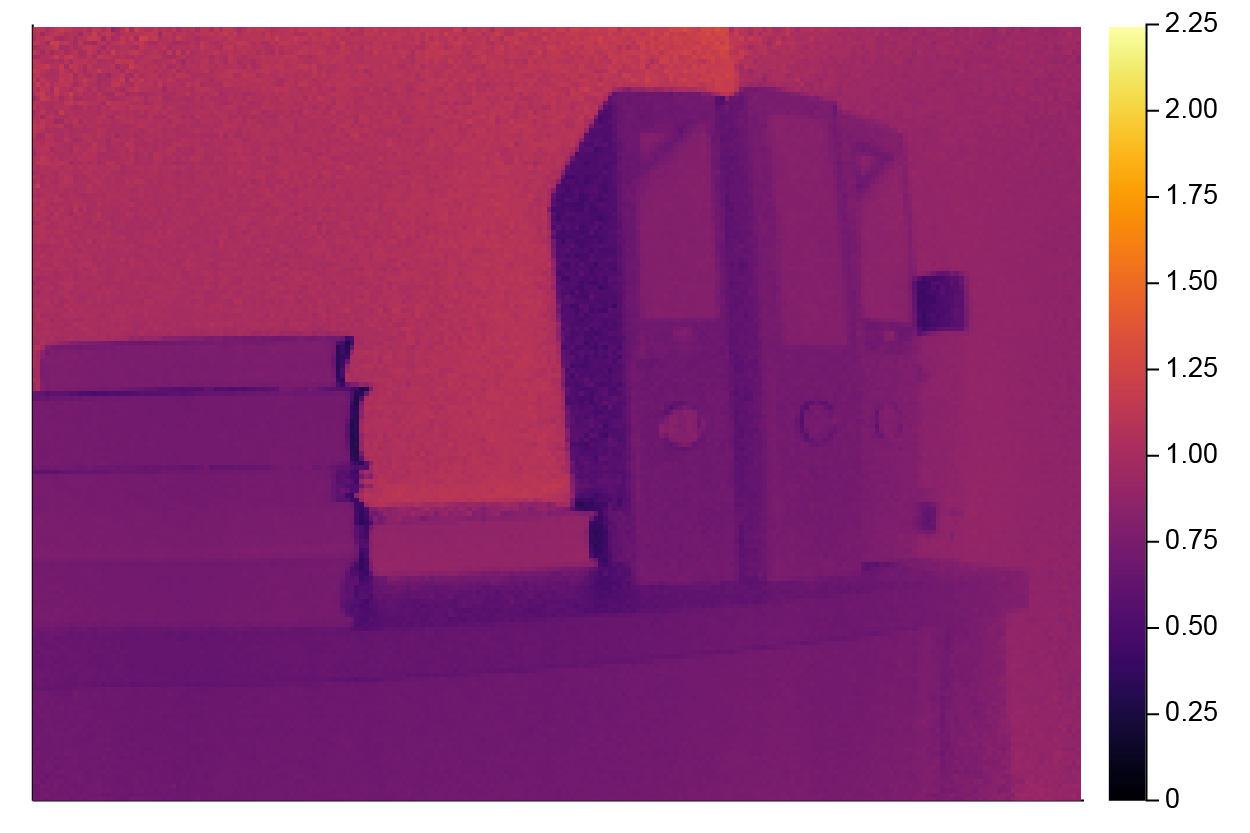
Figure 3.2: Depth images. The depth image is calculated from the two phase difference images shown in Figure 3.1.

4 Experimental Results

In this section, we present some experimental results using raw data captured by an existing standard ToF camera. An example of such data (phase difference images of books scenery) is shown in Figure 3.1; the depth image computed from the difference images via (2.3) is shown in Figure 3.2. From the raw data of the standard ToF camera, we generate the compressive sensing measurements synthetically. For image reconstruction from compressed sensing data we use the block-wise and global $\ell_{1}$-minimization (3.11) as well as block-wise and global TV-regularization(3.12).

4.1 Compressed ToF sensing

For compressive ToF sensing, we initialized the measurement matrices $\mathbf{M}$ (the block circulant matrices; see Section 3.2) randomly with the entries of a random vector generating the partial circulant blocks taking values in $\{-1,1,0\}$ with equal probability. The blocks have size $m\times 14$ which implies that the compression ratio is $14/m$. In the experiments we observed that usually not all blocks of our measurement matrix yield adequate reconstruction properties. This indicates that the size of the single blocks is not large enough to guarantee recovery in each block with high probability. Using bigger blocks would overcome this issue (according to Theorem 3.3), but this is not possible with our camera design. We therefore propose the following alternative strategy. We start with a set of several candidates for the blocks of the measurement matrix from which we choose the ones with the lowest reconstruction error on a set of test images.

For the following results we have chosen the parameters in the FISTA for $\ell_{1}$-minimization and the TV algorithm by hand and did not perform extensive parameter optimization. On most images the parameter choice had a moderate influence on the reconstruction error. Thus we used $\lambda=0.05$ and $\mu=0.1$ for all presented results. For the basis $\boldsymbol{\Psi}$ we use the 2D-Haar wavelet transform and, as described in Section 3.3, we executed the reconstruction block wise with a block size of $28\times 28$. Additionally, for $\ell_{1}$-minimization as well as TV-regularization we performed global reconstruction corresponding to a single block. We use 300 iterations for the block wise $\ell_{1}$-minimization, 1000 for the global $\ell_{1}$-minimization, 100 for block wise TV, and 300 for global TV.

To measure the error between the uncompressed depth image $\mathbf{d}\in\mathds{R}^{n_{1}\times n_{2}}=\mathds{R}^{168\times 224}$ and the reconstructed depth image $\mathbf{d}_{\rm rec}\in\mathds{R}^{168\times 224}$ we use the relative mean absolute error (RMAE) and the peak signal to noise ratio (PSNR) defined by

$$\text{MAE}(\mathbf{d},\mathbf{d}_{\rm rec}) \triangleq\frac{1}{n_{1}n_{2}}\sum_{i=1}^{n_{1}}\sum_{j=1}^{n_{2}}\lvert d_{i,j}-(d_{\rm rec})_{i,j}\rvert$$

$$\text{RMAE}(\mathbf{d},\mathbf{d}_{\rm rec}) \triangleq\frac{\text{MAE}(\mathbf{d},\mathbf{d}_{\rm rec})}{\max_{i,j}\lvert d_{i,j}\rvert}\,$100\text{\,}\mathrm{\char 37\relax}$$$

$$\text{PSNR}(\mathbf{d},\mathbf{d}_{\rm rec}) \triangleq 10\log\left(n_{1}n_{2}\frac{\max_{i,j}(d_{i,j}^{2})}{\sum_{i,j}(d_{i,j}-(d_{\rm rec})_{i,j})^{2}}\right)$\text{\,}\mathrm{dB}$\,.$$

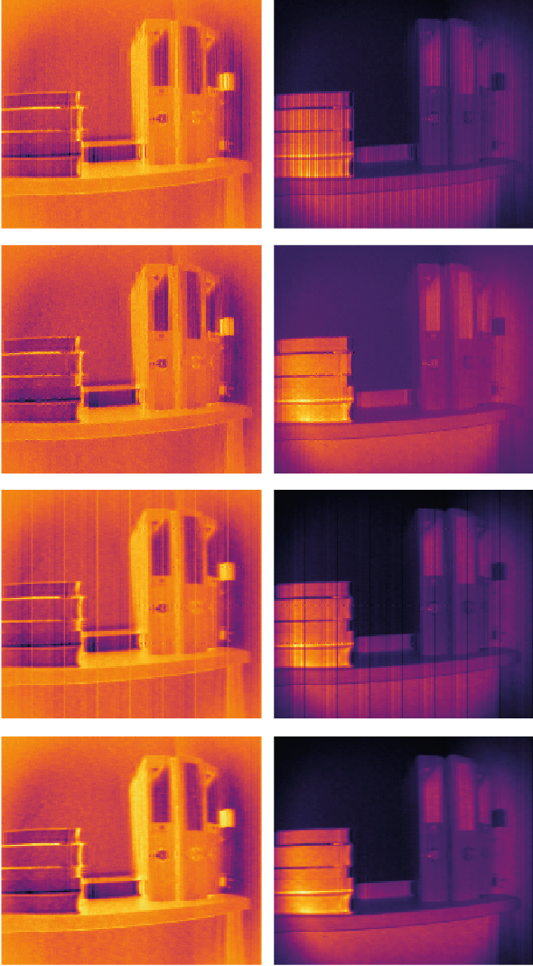
Figure 4.1: Reconstructed phase differences with a compression ratio of $2$. First row: Block-wise $\ell_{1}$-minimization. Second row: Global $\ell_{1}$-minimization. Third row: Block-wise TV-regularization. Fourth row: Global TV-regularization. The original phase differences are shown in Figure 3.1.

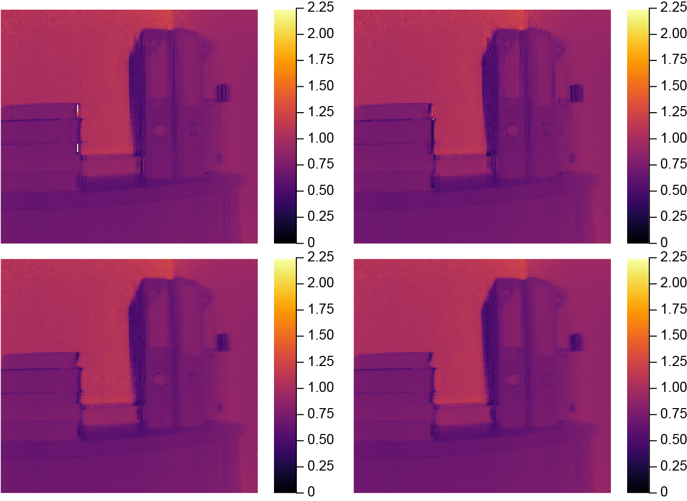
Figure 4.2: Reconstructed depth images with a compression ratio of $2$. Top left: Block-wise $\ell_{1}$-minimization. Top right: Global $\ell_{1}$-minimization. Bottom left: Block-wise TV-regularization. Bottom right: Global TV-regularization. The original depth image is shown in Figure 3.2.

4.2 Numerical results

For the first set of experiments, we consider phase difference images of a scenery with a couple of books and folders shown in Figure 3.1, which is less than 1.2 meters away from the camera (see Figure 3.2). The measured phase images have been calibrated by subtracting a reference image of constant distance (see [12] for additional calibration techniques). Figure 4.1 shows the reconstructed phase difference images from compressed sensing data using a compression ratio of $2$ using block-wise and global $\ell_{1}$-minimization (3.11) and block-wise and global TV-regularization (3.12). The corresponding depth reconstructions are shown in Figure 4.2.

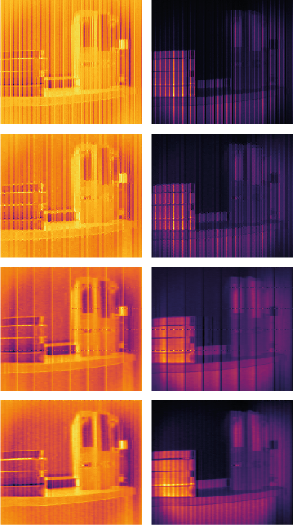
Figure 4.3: Reconstructed phase differences with a compression ratio of $4.7$. First row: Block-wise $\ell_{1}$-minimization. Second row: Global $\ell_{1}$-minimization. Third row: Block-wise TV-regularization. Fourth row: Global TV-regularization. The original phases are shown in Figure 3.1

Figure 4.4: Reconstructed depth images with a compression ratio of $4.7$. Top left: Block-wise $\ell_{1}$-minimization. Top right: Global $\ell_{1}$-minimization. Bottom left: Block-wise TV-regularization. Bottom right: Global TV-regularization. The original depth image is shown in Figure 3.2.

To investigate the reconstruction quality when only using a very small amount of data, we generated a measurement matrix with $m=3$. This results in a compression ratio $14/3$ of around $4.7$. In this example, we also increased the probability for zeros to $2/3$ and the resulting matrix had around $57\text{\,}\mathrm{\char 37\relax}$ zeros. This means that the images can be captured very quickly since zero entries in the measurement matrix imply that the camera can skip the corresponding pixel. The reconstructed phase difference images using block-wise and global $\ell_{1}$-minimization and block-wise and global TV-regularization (3.12) are shown in Figure 4.3 and the corresponding depth reconstructions are shown in Figure 4.4.

4.3 Discussion

Inspection of Figures 4.1 and 4.2 shows that for a compression ratio of $2$ all reconstruction methods perform well. Opposed to that, for the compression ratio $4.7$, global TV-regularization clearly performs best. In a more quantitative way, this is demonstrated in Table 1, where the RMAE and PSNR are shown for depth image reconstructed with the various reconstruction methods. From that table, we see that global TV-regularization in any case yields the smallest RMAE and largest PSNR. For example, for the compression ratio of 4.7, global TV-regularization yields a PSNR of 31.5, opposed to a PSNR of 26.4, 28.0 and 27.3 for block wise $\ell^{1}$-minimization, global $\ell^{1}$-minimization and block wise TV-regularization.

To investigate the dependence of the reconstruction error on the compression ratio more closely, we perform a series of compressed sensing measurements and reconstructions using a set of 24 test images for various compression ratios. The sceneries consist of the books-image and other similar sceneries captured with the ToF camera in an office and an apartment. In Figure 4.5, we show the resulting average RMAE and PSNR using block-wise and global $\ell_{1}$-minimization and block-wise and global TV-regularization. For all test images we use the same FISTA and TV parameters as above. In any case, global TV-regularization clearly outperforms the other reconstruction methods. This is especially prominent in the case of a small number of measurements. Summarizing these findings we can clearly recommend global TV-regularization among the tested sparse recovery algorithms for recovering the depth image from the proposed ToF camera design. Using tools such as dictionary learning or deep learning to find optimal sparsifying transforms is an interesting line of future research.

The reconstruction times for all method are comparable: On a laptop with CPU Intel i5-3427U @ 1.80GHz, performing 100 iterations took about $0.27\text{\,}\mathrm{s}$ for block-wise $\ell_{1}$, $0.42\text{\,}\mathrm{s}$ for global $\ell_{1}$, $0.25\text{\,}\mathrm{s}$ for block-wise TV, and $0.33\text{\,}\mathrm{s}$ for global TV. Finally, note that we also tested to separately recover the four phase images, which we found to yield similar results as for the difference images. Since the latter requires only half of the numerical computations we suggest using sparse recovery of the difference images when computational resources are limited.

Method	RMAE $($\text{\,}\mathrm{\char 37\relax}$)$	PSNR ($\text{\,}\mathrm{dB}$)	CR
FISTA block	1.3	29.8	2
FISTA global	1.2	32.9	2
TV block	1.0	34.4	2
TV global	0.9	34.9	2
FISTA block	2.7	26.4	4.7
FISTA global	2.3	28.0	4.7
TV block	1.8	27.3	4.7
TV global	1.4	31.5	4.7

Table 1: Reconstruction errors and signal to noise ratios for reconstructing the book depth image with compression ratio of $2$ and $4.7$, respectively.

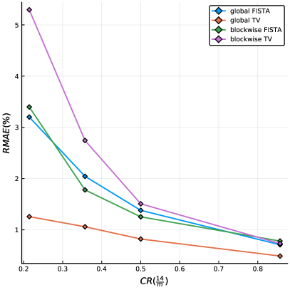
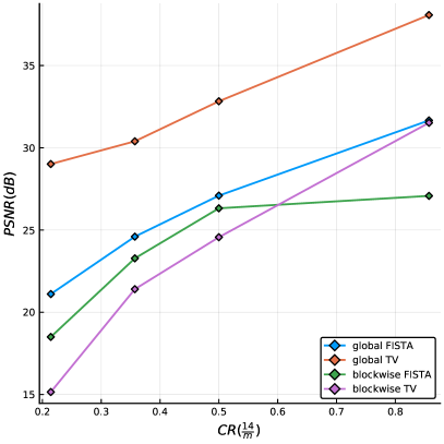
Figure 4.5: Average error analysis. Left: Relative MAE error of the reconstructed depth images depending on the compression ratio $16/m$. Right: Same as on left, but now using the PSNR for evaluating the reconstruction quality.

5 Conclusion

In this paper, we proposed a compressive ToF camera design that reduces the required amount of data to be read-out and transferred. The proposed compressed ToF camera uses measurements within rows of the image which yields a block-diagonal measurement matrix. Random partial circulant matrices as diagonal blocks have been shown to be compatible with current camera architecture. Their asymptotic recovery guarantees do not directly apply in small block sizes. One can increase the block size, which is not really practical for the ToF camera. To overcome this issue, we proposed and implemented strategy to increase the compressed sensing ability of the random partial circulant matrices. Our experimental results clearly demonstrate that it is possible to recover the original images from small measurement blocks.

For image reconstruction we used either blocks-wise or global reconstruction, that both allow to exploit the sparsity of the phase images in the two dimensional wavelet basis ($\ell_{1}$-minimization), or sparsity of the two dimensional gradient (TV-regularization). We empirically found TV-regularization to outperform the wavelet-based $\ell_{1}$-reconstruction which a comparable numerical effort. Future work will be done to further improve the image quality and to increase the reconstruction speed. Among others, for that purpose, we will investigate the use of machine learning in compressed sensing [31].

References

- [1] M. Albrecht. Untersuchung von Photogate-PMD-Sensoren hinsichtlich qualifizierender Charakterisierungsparameter und -methoden. PhD thesis, University of Siegen, 2007.
- [2] S. Antholzer. Nonlinear compressive time-of-flight 3D imaging. Master’s thesis, University of Innsbruck, 2017.
- [3] S. Antholzer, C. Wolf, M. Sandbichler, M. Dielacher, and M. Haltmeier. Compressive time-of-flight imaging. In Sampling Theory and Applications (SampTA), 2017 International Conference on, pages 556–560. IEEE, 2017.
- [4] D. Aschenbrücker. Sparse recovery with random convolutions. Master’s thesis, University of Bonn, 2015.
- [5] A. Beck and M. Teboulle. A fast iterative shrinkage-thresholding algorithm for linear inverse problems. SIAM J. Imaging Sci., 2(1):183–202, 2009.
- [6] J. Bourgain, S. Dilworth, K. Ford, S. Konyagin, and D. Kutzarova. Explicit constructions of RIP matrices and related problems. Duke Math. J., 159(1):145–185, 2011.
- [7] T. Cai and A. Zhang. Sparse representation of a polytope and recovery of sparse signals and low-rank matrices. IEEE Trans. Inf. Theory, 60:122 – 132, 2014.
- [8] E. Candes and T. Tao. Near-optimal signal recovery from random projections: Universal encoding strategies? IEEE Trans. Inf. Theory, 52(12):5406–5425, 2006.
- [9] E. J. Candès, Y. C. Eldar, D. Needell, and P. Randall. Compressed sensing with coherent and redundant dictionaries. Appl. Comput. Harmon. Anal., 31(1):59–73, 2011.
- [10] E. J. Candès, J. K. Romberg, and T. Tao. Stable signal recovery from incomplete and inaccurate measurements. Comm. Pure Appl. Math., 59(8):1207–1223, 2006.
- [11] A. Chambolle and T. Pock. A first-order primal-dual algorithm for convex problems with applications to imaging. J. Math. Imaging Vision, 40(1):120–145, 2011.
- [12] M. H. Conde. Compressive Sensing for the Photonic Mixer Device: Fundamentals, Methods and Results. Springer Vieweg, 2017.
- [13] D. Droeschel, D. Holz, and S. Behnke. Multi-frequency phase unwrapping for time-of-flight cameras. In 2010 IEEE/RSJ International Conference on Intelligent Robots and Systems, pages 1463–1469, 2010.
- [14] S. Foix, G. Alenya, and C. Torras. Lock-in time-of-flight (tof) cameras: A survey. IEEE Sensors Journal, 11(9):1917–1926, 2011.
- [15] S. Foucart and H. Rauhut. A mathematical introduction to compressive sensing. Applied and Numerical Harmonic Analysis. Birkhäuser/Springer, New York, 2013.
- [16] M. Grasmair, M. Haltmeier, and O. Scherzer. Necessary and sufficient conditions for linear convergence of -regularization. Comm. Pure Appl. Math., 64(2):161–182, 2011.
- [17] M. Haltmeier. Stable signal reconstruction via -minimization in redundant, non-tight frames. IEEE Trans. Signal Process., 61(2):420–426, 2013.
- [18] M. E. Hansard, S. Lee, O. Choi, and R. Horaud. Time-of-Flight Cameras – Principles, Methods and Applications. Springer Briefs in Computer Science. Springer, 2013.
- [19] G. A. Howland, P. Zerom, R. W. Boyd, and J. C. Howell. Compressive sensing lidar for 3D imaging. In CLEO: 2011 - Laser Science to Photonic Applications, pages 1–2, May 2011.
- [20] M. A. Iwen. Simple deterministically constructible rip matrices with sublinear Fourier sampling requirements. In 2009 43rd Annual Conference on Information Sciences and Systems, pages 870–875, 2009.
- [21] L. Jacques, P. Vandergheynst, A. Bibet, V. Majidzadeh, A. Schmid, and Y. Leblebici. Cmos compressed imaging by random convolution. In Acoustics, Speech and Signal Processing, 2009 International Conference on, pages 1113–1116. IEEE, 2009.
- [22] A. Kadambi and P. T. Boufounos. Coded aperture compressive 3-d lidar. In 2015 IEEE International Conference on Acoustics, Speech and Signal Processing (ICASSP), pages 1166–1170, April 2015.
- [23] N. Katic, M. H. Kamal, A. Schmid, P. Vandergheynst, and Y. Leblebici. Compressive image acquisition in modern CMOS IC design. Int. J. Circ. Theor. and App., 43(6):722–741, 2015.
- [24] A. Kirmani, A. Colaço, F. N. C. Wong, and V. K. Goyal. Codac: A compressive depth acquisition camera framework. In 2012 IEEE International Conference on Acoustics, Speech and Signal Processing (ICASSP), pages 5425–5428, 2012.
- [25] F. Krahmer, C. Kruschel, and M. Sandbichler. Total variation minimization in compressed sensing. arXiv preprint arXiv:1704.92195, 2017.
- [26] F. Krahmer, S. Mendelson, and H. Rauhut. Suprema of chaos processes and the restricted isometry property. Comm. Pure Appl. Math., 67(11):1877–1904, 2014.
- [27] F. Krahmer, D. Needell, and R. Ward. Compressive sensing with redundant dictionaries and structured measurements. SIAM J. Math. Anal., 47(6):4606–4629, 2015.
- [28] F. Krahmer and R. Ward. Stable and robust sampling strategies for compressive imaging. IEEE Trans. Image Process., 23(2):612–622, 2014.
- [29] R. Lange. 3D Time-of-Flight Distance Measurement with Custom Solid-State Image Sensors in CMOS/CCD-Technology. PhD thesis, University of Siegen, 2000.
- [30] K. Li, L. Gan, and C. Ling. Convolutional compressed sensing using deterministic sequences. IEEE Trans. Signal Process., 61(3):740–752, 2013.
- [31] A. Mousavi and R. G. Baraniuk. Learning to invert: Signal recovery via deep convolutional networks. arXiv:1701.03891, 2017.
- [32] C. Poon. On the role of total variation in compressed sensing. SIAM J. Imaging Sci., 8(1):682–720, 2015.
- [33] H. Rauhut, J. Romberg, and J. A. Tropp. Restricted isometries for partial random circulant matrices. Appl. Comput. Harmon. Anal., 32(2):242–254, 2012.
- [34] H. Rauhut, K. Schnass, and P. Vandergheynst. Compressed sensing and redundant dictionaries. IEEE Trans. Inf. Theory, 54(5):2210 –2219, 2008.
- [35] O. Scherzer, M. Grasmair, H. Grossauer, M. Haltmeier, and F. Lenzen. Variational methods in imaging, volume 167 of Applied Mathematical Sciences. Springer, New York, 2009.
- [36] C. Wolf. Framework for compressed sensing in time-of-flight based 3D imaging. Master’s thesis, University of Innsbruck, 2016.
- [37] R. Zimmermann and W. Fichtner. Low-power logic styles: Cmos versus pass-transistor logic. IEEE J. Solid-State Circuits, 32(7):1079–1090, 1997.