Jointly Tracking and Separating Speech Sources Using Multiple Features and the generalized labeled multi-Bernoulli Framework

Abstract

This paper proposes a novel joint multi-speaker tracking-and-separation method based on the generalized labeled multi-Bernoulli (GLMB) multi-target tracking filter, using sound mixtures recorded by microphones. Standard multi-speaker tracking algorithms usually only track speaker locations, and ambiguity occurs when speakers are spatially close. The proposed multi-feature GLMB tracking filter treats the set of vectors of associated speaker features (location, pitch and sound) as the multi-target multi-feature observation, characterizes transitioning features with corresponding transition models and overall likelihood function, thus jointly tracks and separates each multi-feature speaker, and addresses the spatial ambiguity problem. Numerical evaluation verifies that the proposed method can correctly track locations of multiple speakers and meanwhile separate speech signals.

Index Terms—  multi-speaker tracking, multi-feature extraction, speech separation, microphone array processing, GLMB filter.

1 Introduction

Multi-speaker tracking using microphones is an important task in smart environments such as automatic camera steering in video conferencing. Numerous acoustic multi-speaker tracking algorithms can be found in the literature [1, 2, 3, 4], using various techniques such as mutual information or cross-correlation for spatial localization, and particle filtering for speaker tracking. Generic multi-target tracking filters [5, 6, 7, 8] can also be implemented to track multiple speakers online when provided with speaker location estimates as multi-target observations. These existing implementations of multi-speaker tracking methods however, usually track only spatial locations of respective speakers. Moreover, spatial tracking has the ambiguity problem when speakers are spatially close to each other, because by relying on the location information alone, the tracking filters would take them as a single speaker, hence unable to correctly identify and separate the sound sources in the mixture.

Separating original source signals from the mixtures recorded by microphones has also a wide range of applications such as automatic meeting transcription and speaker recognition. Many blind source separation (BSS) methods have been developed [9, 10, 11, 12], based on the independent component analysis (ICA) or time-frequency masking (TFM) techniques. However, it can be challenging for some BSS methods to continuously separate moving sources. Thus the location-based source separation methods, e.g. the wideband beamforming methods [13, 14], are often employed as an additional source separation step after obtaining the location tracking results.

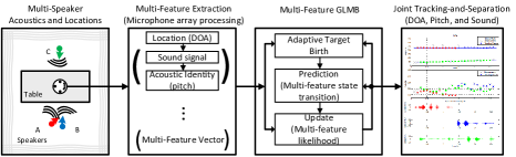
Fig. 1: System overview.

In this paper, we propose a systematic multi-feature tracking-and-separation framework based on the generalized labeled multi-Bernoulli (GLMB) filter [6, 7, 8]. As shown in Fig. 1, we first obtain multiple speaker features from sound mixtures by detecting locations of all candidate speakers, extracting their corresponding speech signals and estimating the related acoustic identities (pitches). Each extracted vector of associated speaker features of a candidate speaker, i.e. the location, pitch and the corresponding speech signals, can be treated as an integral multi-feature target observation. The set of multi-feature vectors forms the multi-target multi-feature observations, which are then tracked in the proposed multi-feature GLMB. Moreover, since the standard implementations of the GLMB framework [6, 7, 8] track only one feature, necessary adaptations are required to support multi-feature tracking. We categorize the location and pitch as “transitioning” features, while the non-stationary sound signal as a “non-transitioning” feature. In the multi-feature GLMB recursion, transitioning features have their own first-order Markov transition models and are directly used for track confirmation in the update step, while the non-transitioning feature is zeroed in the prediction step and assigned with associated extracted sound in the update step. We also propose new state transition function and measurement likelihood function for multiple transitioning features. The multi-feature GLMB tracking filter produces labeled tracks for respective speakers, the corresponding pitch estimates, as well as the separated sound signals. Furthermore, it also addresses the ambiguity problem because when speakers locate closely, their pitch information can be used to separate them in the multi-feature GLMB tracking algorithm, and vice versa.

2 Speaker Feature Extraction

2.1 Speaker Localization

We use a circular microphone array in this paper. Denote the sound signals captured by the microphone array as $x_{j}(t)$ and locations of microphones as $\vec{m}_{j}$, where $t\in\mathbb{R},~{}j=1,...,M$, integer $M$ is the number of microphones. We formulate a multi-channel implementation of the generalized cross-correlation - phase transform (GCC-PHAT) method [15], which we refer to as the MCC-PHAT:

$$\xi^{\mathrm{mcc-phat}}(k,\varsigma)\triangleq\prod\limits_{(i,j)\in P}\xi_{ij}^{\mathrm{gcc-phat}}(k,\tau_{ij}(\varsigma)),$$ (1)

where

$$\xi_{ij}^{\mathrm{gcc-phat}}(k,\tau_{ij}(\varsigma))=\int_{-\infty}^{+\infty}\Xi_{ij}^{\mathrm{gcc-phat}}(k,f)\cdot e^{\mathrm{i}2\pi f\tau_{ij}(\varsigma)}df,$$ (2)

and

$$\Xi_{ij}^{\mathrm{gcc-phat}}(k,f)=\frac{X_{i}(k,f)\cdot X_{j}^{\star}(k,f)}{|X_{i}(k,f)\cdot X_{j}^{\star}(k,f)|}.$$ (3)

Here $\mathrm{i}=\sqrt{-1}$, $[\cdot]^{\star}$ the complex conjugate operation, $X_{i}(k,f)$ and $X_{j}(k,f)$ are respectively the short-time Fourier transforms of microphone signals $x_{i}(\cdot)$ and $x_{j}(\cdot)$ at time frame $k$. (In practice, sound signals are discretized into $x_{i}(n),~{}n\in\mathbb{Z}$ at a sampling frequency $f_{s}=48000$Hz, thus the short-time FFT is used in (3), and the integration in (2) becomes a summation.)

Time difference $\tau_{ij}$ is a function of speaker direction of arrival (DOA) $\varsigma\in[0,360^{\circ})$ from a distance of $r=1$m (far-field)

$$\tau_{ij}(\varsigma)=(\|\vec{\wp}(\varsigma)-\vec{m}_{i}\|-\|\vec{\wp}(\varsigma)-\vec{m}_{j}\|)/v,$$ (4)

$$\vec{\wp}(\varsigma)=[r\cdot\cos\varsigma,~{}r\cdot\sin\varsigma].$$ (5)

To avoid spatial alias, the set of microphone pairs $P$ is

$$P=\{(i,j)\;|\|\vec{m}_{i}-\vec{m}_{j}\|<v/f_{max});\;1\leq i<j\leq M\},$$ (6)

where $v=343$m/s is the velocity of sound, and $f_{max}=3600$Hz is the maximum signal frequency considered.

In this paper, we use only one circular microphone array in the azimuth plane. (Cartesian locations of speakers can be obtained using multiple microphone arrays.) The set of estimated DOAs of candidate speakers are denoted as $\hat{\Theta}_{k}$ at time $k$:

$$\hat{\Theta}_{k}=\{\hat{\varsigma}_{k,i}~{}|~{}{i}=1,\dots,{N_{k}}\},$$ (7)

where $\hat{\varsigma}_{k,i}$ correspond to the local peaks of $\xi^{\mathrm{mcc-phat}}(k,\cdot)$, and integer $N_{k}\geq 0$ denotes the number of detected speakers (accounting for spurious estimates from reflections, and miss detections due to non-stationary or competing speech signals) at frame $k$. $N_{k}=0$ indicates that no candidate speaker is detected and thus $\hat{\Theta}_{k}=\emptyset$. Assuming in general that the spurious estimates and miss detections exhibit no temporal consistency from one time frame to the next, while the estimates from true speakers follow a kinematic model, tracking filters [1, 3, 6, 7, 8] can be applied to track speaker locations. Such approach is also applied for tracking multiple features as shown in Section 3.

2.2 Sound Extraction

Speech signals from the DOA estimates $\hat{\varsigma}_{k,i}$ can then be extracted from the sound mixtures recorded by microphones. Here we implement the wideband weighted least square (WLS) beamforming method [14] for sound extraction.

The WLS beamformer uses the filter-and-sum structure, and has $J_{t}=32$ taps in each channel. Its mainlobe steers to the speaker DOA $\hat{\varsigma}_{k,i}$, and the corresponding sidelobe ranges from $\hat{\varsigma}_{k,i}+15^{\circ}$ to $\hat{\varsigma}_{k,i}-15^{\circ}$. The frequency range used is [20, 8000]Hz.

The real-valued $(J_{t}\cdot M)\times 1$ optimal weight vector $\mathbf{w}_{k,i}$ for a DOA $\hat{\varsigma}_{k,i}$ is obtained according to the wideband WLS beamformer [14] and using the microphone locations $\vec{m}_{j}$, then the extracted sound signal at time frame $k$ can be calculated from:

$$\hat{s}_{k,i}\big{(}n)=\mathbf{w}_{k,i}^{T}~{}\mathbf{x}(n),$$ (8)

where $[\cdot]^{T}$ is the matrix transpose, and

$${\mathbf{x}}(n)\!=\!\begin{bmatrix}\mathbf{x}_{0}(n),\dots,\mathbf{x}_{j_{t}}(n),\dots,\mathbf{x}_{J_{t}-1}(n)\end{bmatrix}^{T}\!\!\!,~{}j_{t}\in\![0,J_{t}\!-\!1]$$ (9)

$$\mathbf{x}_{j_{t}}(n)=\begin{bmatrix}{x}_{1}(n+j_{t}),\dots,{x}_{j}(n+j_{t}),\dots,{x}_{M}(n+j_{t})\end{bmatrix}.$$ (10)

2.3 Acoustic Identity

The extracted sound $\hat{s}_{k,i}$ that corresponds to a speaker location $\hat{\varsigma}_{k,i}$ can further be used to extract speaker’s acoustic identity, e.g. pitch, Gaussian Mixture Model (GMM) [16] parameters, etc. In this paper we use the pitch as a simple acoustic identity, as pitch can be estimated from a short segment of voiced sound, different speakers usually have different pitch, and pitch of a speaker is usually distributed within a limited range. Numerous pitch estimation methods can be found in the literature. Here we employ the PEFAC (Pitch Estimation Filter with Amplitude Compression) method [17] and use the averaged estimate of each frame, which we denote as $\hat{F_{0}}_{k,i}$.

From (7) and (8), the vector of associated location, pitch and sound of each candidate speaker at frame $k$ form a multi-feature observation ${z}_{k,i}\triangleq(\hat{\varsigma}_{k,i},\hat{{F_{0}}}_{k,i},\hat{s}_{k,i})$. The multi-target multi-feature observation is thus

$$Z_{k}\triangleq\{z_{k,i}~{}|~{}i=1,...,N_{k}\},$$ (11)

where $Z_{k}=\emptyset$ when $N_{k}=0$.

Instead of using the location estimates alone, we jointly extract and track the location, pitch and sound features in the extended multi-feature GLMB filter as follows.

3 Multi-feature GLMB

The multi-feature GLMB random finite set (RFS) $\mathbf{X}\triangleq\{(\mathrm{x}_{i},\ell_{i})~{}|~{}i\in\mathbb{N}\}$ is a labeled RFS with state space $\mathbb{X}$ (here $\mathrm{x}_{i}\triangleq(\zeta_{i},{F_{0}}_{i},s_{i})\in\mathbb{X}$ is the multi-feature target state vector, where $\zeta_{i},{F_{0}}_{i},s_{i}$ denote the associated location and pitch feature states as well as the sound signal, respectively), and label space $\mathbb{L},(\ell_{i}\in\mathbb{L})$, where the labels are unique, i.e. $\ell_{i}\neq\ell_{i^{\prime}},~{}\forall i\neq i^{\prime}$. Its probability density in the $\delta$-GLMB form is given as [6]

$$\mathbf{\pi}(\mathbf{X})=\Delta(\mathbf{X})\!\!\!\!\sum_{(I,\xi)\in\mathcal{F}(\mathbb{L})\times\Xi}\omega^{(I,\xi)}\delta_{I}(\mathcal{L(}\mathbf{X}))\left[p^{(\xi)}\right]^{\mathbf{X}},$$ (12)

where $\omega^{(I,\xi)}$ is the probability of the hypothesis $(I,\xi)$, $I$ is a set of labels, $\xi$ represents a history of association map between targets and observations. $p^{(\xi)}$ is the probability distribution of a target state, $\Delta(\mathbf{X})$ is the distinct label indicator, $\delta_{I}(\mathcal{L(}\mathbf{X}))$ indicates whether the set of labels in $\mathbf{X}$ matches that of $I$. The $\delta$-GLMB is completely characterized by the set of parameters $\{(\omega^{(I,\xi)},p^{(\xi)}):(I,\xi)\in\mathcal{F}(\mathbb{L})\times\Xi\}$. (Reader are encouraged to read [6, 7, 8] and their references for detailed studies of the (G)LMB and $\delta$-GLMB RFS tracking filters.)

The multi-feature GLMB recursion also consists of the multi-object “update” step based on Bayes inference and the Chapman-Kolmogorov [18] “prediction” step based on the state transition models.

3.1 Multi-feature GLMB Recursion: Update

If the current RFS prediction density is a $\delta$-GLMB of the form (12), using the current multi-feature observation $Z$ as defined in (11), the posterior density is a $\delta$-GLMB [7], i.e.

$$\mathbf{\pi}\!(\mathbf{X}|Z)=$$ (13)

$$\Delta\!(\mathbf{X})\!\!\!\!\!\!\!\!\sum_{(I,\xi)\in\mathcal{F}\!(\mathbb{L})\!\times\!\Xi}\;\sum\limits_{\theta\in\Theta\!(I)}\!\!\!\!\omega^{\!(I,\xi,\theta\!)\!}(Z)\delta_{\!I\!}(\mathcal{L\!(}\mathbf{X})\!)\!\!\left[p^{\!(\xi,\theta)\!}(\cdot|Z)\right]^{\!\mathbf{X}},$$

where $\Theta(I)$ denotes the subset of current association maps with domain $I$, and standard derivations of $\omega^{(I,\xi,\theta)\!}(Z)$ and $p^{\!(\xi,\theta)\!}(\mathrm{x},\ell|Z)$ are provided in [7]. (For denotation simplicity we drop the subscript $k$ here.)

Following the definitions in [7], clutter is assumed Poisson with an average of 0.044 clutter points per scan, i.e. the localization method in Section 2.1 produces almost clean location estimates in low reverberation. The probability of a target state being detected is $p_{D}=0.98\mathcal{N}({F_{0}};280,30^{2})/\mathcal{N}(280;280,30^{2})$.

In this paper, $\mathrm{g}({z}_{\theta(\ell)}|\mathrm{x},\ell)$ denotes the multi-feature likelihood for the measurement ${z}_{\theta(\ell)}\in Z$ being generated by $(\mathrm{x},\ell)=((\zeta,{F_{0}},s),\ell)$, where $s=\hat{s}_{\theta(\ell)}$ after update. Sound separation for respective speakers over time is achieved by concatenating sound signals $s$ of the same target label. Assuming that the transitioning features (location and pitch) are statistically independent, the proposed multi-feature likelihood function is:

$$\mathrm{g}({z}_{\theta(\ell)}|\mathrm{x},\ell)\triangleq\mathrm{g}(\hat{\varsigma}_{\theta(\ell)}|\zeta,\ell)\cdot\mathrm{g}(\hat{{F_{0}}}_{\theta(\ell)}|{F_{0}},\ell),$$ (14)

where $\mathrm{g}(\hat{\varsigma}_{\theta(\ell)}|\zeta,\ell)=\mathcal{N}(\hat{\varsigma}_{\theta(\ell)};\zeta,\sigma_{\varsigma}^{2})$ and $\mathrm{g}(\hat{{F_{0}}}_{\theta(\ell)}|{F_{0}},\ell)=\mathcal{N}(\hat{{F_{0}}}_{\theta(\ell)};{F_{0}},\sigma_{F_{0}}^{2})$ in this paper. $\sigma_{\varsigma}=2^{\circ}$ and $\sigma_{F_{0}}=10$Hz are the standard deviations of the observation of the location and pitch, respectively. After update, the maximum a posteriori (MAP) estimate of the cardinality (number of speakers) is chosen, and the highest weighted corresponding hypothesis is used for the multi-target multi-feature tracking results.

3.2 Multi-feature GLMB Recursion: Prediction

If the current RFS filtering density from its previous update step is a $\delta$-GLMB of the form (12), the prediction density to the next time is a $\delta$-GLMB given as [7]

$$\mathbf{\pi}_{\!+} (\mathbf{X}_{\!+\!})=\Delta(\mathbf{X}_{\!+})\!\!\!\!\!\!\!\sum_{(I_{+},\xi)\in\mathcal{F}(\mathbb{L}_{+})\times\Xi}\!\!\!\!\omega_{+}^{(I_{+},\xi)}\delta_{I_{+\!}}(\mathcal{L(}\mathbf{X}_{\!+}))\!\left[p_{+}^{(\xi)\!}\right]^{\!\mathbf{X}_{+}},$$ (15)

where standard derivations of $\omega_{+}^{(I_{+},\xi)}$ and $p_{+}^{(\xi)}(\mathrm{x},\ell)$ can be found in [7]. $[\cdot]_{+}$ stands for prediction. The survival probability is $p_{S}(\cdot,\ell)=0.75$.

Using the assumption that the transitioning features are statistically independent, the proposed state transition function for the multi-feature GLMB is:

$$\mathrm{f}(\mathrm{x}|\cdot,\ell)=1_{\mathrm{x}}(\zeta)\cdot\mathrm{f}(\mathrm{\zeta}|\cdot,\ell)~{}\cdot~{}1_{\mathrm{x}}({F_{0}})\cdot\mathrm{f}({F_{0}}|\cdot,\ell),$$ (16)

where the inclusion function is defined as

$$1_{Y}(X)\triangleq\left\{\begin{array}[]{l}1,\text{ if }X~{}\text{is included in}~{}Y\\ 0,\text{ otherwise}.\end{array}\right.$$ (17)

We assume the motion of the speaker DOA follows the Langevin process [19, 1, 3], which is also a first-order Markov model:

$$\mathrm{f}(\mathrm{\zeta}|\zeta^{\prime},\ell)=\begin{bmatrix}1&t_{\Delta}\\ 0&e^{-\beta_{\zeta}\cdot t_{\Delta}}\end{bmatrix}\cdot\zeta^{\prime}+w_{\zeta}\cdot\begin{bmatrix}0\\ \sigma_{\zeta}~{}\sqrt[]{1-e^{-2\beta_{\zeta}\cdot t_{\Delta}}}\end{bmatrix},$$ (18)

$\zeta=[\varsigma,\dot{\varsigma}]^{T}$, $\dot{\varsigma}$ is the velocity of DOA $\varsigma$. $t_{\Delta}=0.1$s is the time step, $w_{\zeta}$ follows the normal distribution, i.e. $w_{\zeta}\sim\mathcal{N}(\cdot;0,1)$. Model parameters $\beta_{\zeta}=0.2\mathrm{s}^{-1}$ and $\sigma_{\zeta}=10^{\circ}/\mathrm{s}$ are respectively the rate constant and the steady-state root-mean-square velocity for the random motions of speakers.

We also assume that the pitch of a speaker follows a simple normal distribution around its previous estimate. Thus the state transition function for pitch is:

$$\mathrm{f}({F_{0}}|\mathrm{F_{0}}^{\prime},\ell)=\mathcal{N}({{F_{0}}};{F_{0}}^{\prime},\tilde{\sigma}_{F_{0}}^{2}),$$ (19)

where $\tilde{\sigma}_{F_{0}}=30$Hz is the standard deviation for the transition of pitch. Adaptive measurement-driven target births are generated [8, 20]. New target births are assumed to follow normal distributions around the previous measurement, where the standard deviation is $5^{\circ}$ for the DOA, and $30$Hz for the pitch, respectively. The non-stationary sound signals are treated as the non-transitioning feature, thus targets carry no sound in prediction until the next update step of the multi-feature GLMB recursion.

4 Numerical Studies

4.1 Experiment Setup

This section verifies and demonstrates the performance of the proposed multi-feature GLMB framework in the scenario of three speakers.

The setup is as shown in the left panel of Fig. 1, where the room dimensions are $3.4(W)\times 7.6(L)\times 2.7(H)\mathrm{m}^{3}$, the microphone array locates at [1.2, 3.9, 1.5]m, which is composed of $M=8$ microphones evenly distributed on a circle with a diameter of $0.1$m. For clarity, we choose an anechoic scenario that Speaker A (male) and B (female) both locate at DOA of $232.1^{\circ}$ while Speaker C (female) moves from DOA of $40^{\circ}$ to $75^{\circ}$, with respect to the center of the microphone array. Fig. 2 plots the normalized ground truth speech signals of respective speakers as well as their mixture captured by one of the microphones. Obviously, using location (DOA) information alone, standard implementations of tracking methods can only take Speaker A and B as a same speaker. (The scenario when closely located speakers talk concurrently is not in the scope of this paper.)

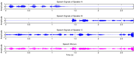
Fig. 2: Ground truth (top three panels) of the normalized speech signals of three speakers (one male and two female), and their mixture at one of the microphones (bottom panel).

4.2 Test Results

Fig. 3 provides the ground truth locations, estimated speaker locations, pitch and separated sound signals. The top panel depicts the ground truth locations in straight line segments, our estimated locations in symbol “$\times$” and tracking results in solid colored symbols. Different colored symbols represent different speakers. From the ground truth, there are two separate lines of locations. Thus using location information alone, apparently the tracking filters can only detect two speakers. However, by considering also the pitch information, our proposed method has correctly found three speakers. The second top panel shows the pitch estimates and tracking results associated with the location estimates and tracking results in the top panel. We can see in these two panels that the associated location and pitch estimates have spurious errors that do not follow consistent kinematic patterns over time, thus are filtered by the GLMB tracker. We can also see that the tracking filter requires two time steps to confirm one new track. This is reasonable as we use the measurement-driven birth model [20] for adaptive target births. The pitch estimates of different speakers fluctuate at different levels over time, and there is a significant jump in pitch level at time of around $1.4$s, which helps the tracker to confirm a new speaker starting at $1.5$s. The bottom three panels of Fig. 3 plots the extracted sound signals for respective speakers. Comparing with Fig. 2, we can see that most of speech signals are recovered for each speaker. Thus our proposed multi-feature GLMB tracking-and-separation method can jointly track and separate multiple speakers.

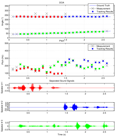
Fig. 3: Joint tracking and separation results from proposed methods. Top two panels show the estimation and tracking results of speakers’ location and pitch. Bottom three panels show the corresponding separated sound signals.

The location tracking accuracy is evaluated using the Optimal Sub-pattern Assignment (OSPA) metric [21], with the cut-off parameter of $5^{\circ}$ and the order parameter of $1$. Thus cardinality estimation error of 1 out of 2 contributes to an OSPA error of $\frac{5}{2}^{\circ}$. Fig. 4 shows that the overall OSPA location tracking errors are within $5^{\circ}$, and the multi-feature GLMB achieves comparable location tracking accuracy with the standard GLMB.

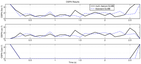
Fig. 4: OSPA measure of the DOA tracking results, i.e. the overall OSPA errors (top), the contribution of DOA errors (middle), and the contribution of cardinality errors (bottom).

The quality of the separated sound signals are evaluated using the PEASS metric [22], compared with the ground truth signals. The results are provided in Tab. 1. We also compare the performance with two blind speech separation methods, i.e. the Underdetermined Convolutive Blind Source Separation (UCBSS) [12] and the Degenerative Unmixing Estimation Technique (DUET) [9]. We can see that using the blind separation techniques, the speaker 1 and speaker 2 are regarded as one speaker. Thus the separated sound signals for speaker $<1,2>$ are compared with the mixture of Speaker A and Speaker B. In general the DUET and UCBSS methods obtain close Overall Perceptual Scores (OPS). The DUET method seems to provide more consistent performance than UCBSS when comparing the Target-related Perceptual Score (TPS) and the Artifacts-related Perceptual Scores (APS), but UCBSS has significantly higher Interference-related Perceptual Score (IPS) than DUET. Overall, our proposed method provides consistent and superior performance for the three separated speakers, according to all the perceptual scores.

Table 1: PEASS evaluation results for speech separation, using the proposed method, and the UCBSS, DUET methods.

Method	Speaker	OPS	TPS	IPS	APS
Proposed	$1$	48.75	57.03	71.19	49.11
	$2$	32.69	29.35	72.06	35.61
	$3$	36.02	35.73	65.65	37.71
UCBSS	$<1,2>$	18.66	45.84	43.21	24.33
	$3$	25.00	6.10	83.97	3.50
DUET	$<1,2>$	18.73	38.82	16.38	50.43
	$3$	24.97	51.16	32.40	44.32

5 Conclusion and Future Work

This paper presents the novel systematic implementation of multi-feature GLMB tracking method that not only can jointly track multiple speakers and separate sound signals from speech mixtures, but also resolve the ambiguity of location tracking when speakers locate spatially close. It treats the vector of candidate speaker location, pitch and sound as a multi-feature target observation and jointly extracts and tracks these features in the Bayes RFS recursion. Experimental results demonstrate encouraging results in the studied scenario. For future work, further improvement is still possible, e.g. by applying more complicated microphone setup, selecting different speaker features, or improving the feature extraction methods.

References

- [1] Darren B Ward, Eric Lehmann, Robert C Williamson, et al., “Particle filtering algorithms for tracking an acoustic source in a reverberant environment,” IEEE Transactions on Speech and Audio Processing, vol. 11, no. 6, pp. 826–836, 2003.
- [2] Ba-Ngu Vo, Sumeetpal Singh, and Wing Kin Ma, “Tracking multiple speakers using random sets,” in IEEE International Conference on Acoustics, Speech, and Signal Processing, 2004. Proceedings.(ICASSP’04). IEEE, 2004, vol. 2, pp. ii–357.
- [3] Wing-Kin Ma, Ba-Ngu Vo, Sumeetpal S Singh, and Adrian Baddeley, “Tracking an unknown time-varying number of speakers using tdoa measurements: a random finite set approach,” IEEE Transactions on Signal Processing, vol. 54, no. 9, pp. 3291–3304, 2006.
- [4] Fotios Talantzis, “An acoustic source localization and tracking framework using particle filtering and information theory,” IEEE Transactions on Audio, Speech, and Language Processing, vol. 18, no. 7, pp. 1806–1817, 2010.
- [5] Ba-Tuong Vo, Ba-Ngu Vo, and Antonio Cantoni, “Analytic implementations of the cardinalized probability hypothesis density filter,” IEEE Transactions on Signal Processing, vol. 55, no. 7, pp. 3553–3567, 2007.
- [6] Ba-Tuong Vo and Ba-Ngu Vo, “Labeled random finite sets and multi-object conjugate priors,” IEEE Transactions on Signal Processing, vol. 61, no. 13, pp. 3460–3475, 2013.
- [7] Ba-Ngu Vo, Ba-Tuong Vo, and Dinh Phung, “Labeled random finite sets and the bayes multi-target tracking filter,” IEEE Transactions on Signal Processing, vol. 62, no. 24, pp. 6554–6567, 2014.
- [8] Stephan Reuter, Ba-Tuong Vo, Ba-Ngu Vo, and Klaus Dietmayer, “The labeled multi-bernoulli filter,” IEEE Transactions on Signal Processing, vol. 62, no. 12, pp. 3246–3260, 2014.
- [9] Ozgur Yilmaz and Scott Rickard, “Blind separation of speech mixtures via time-frequency masking,” IEEE Transactions on Signal Processing, vol. 52, no. 7, pp. 1830–1847, 2004.
- [10] Hiroshi Sawada, Ryo Mukai, Shoko Araki, and Shoji Makino, “A robust and precise method for solving the permutation problem of frequency-domain blind source separation,” IEEE Transactions on Speech and Audio Processing, vol. 12, no. 5, pp. 530–538, 2004.
- [11] Taesu Kim, Hagai T Attias, Soo-Young Lee, and Te-Won Lee, “Blind source separation exploiting higher-order frequency dependencies,” IEEE transactions on audio, speech, and language processing, vol. 15, no. 1, pp. 70–79, 2007.
- [12] Vaninirappuputhenpurayil Gopalan Reju, Soo Ngee Koh, and Yann Soon, “Underdetermined convolutive blind source separation via time–frequency masking,” IEEE Transactions on Audio, Speech, and Language Processing, vol. 18, no. 1, pp. 101–116, 2010.
- [13] Simon Doclo and Marc Moonen, “Design of broadband beamformers robust against gain and phase errors in the microphone array characteristics,” IEEE Transactions on Signal Processing, vol. 51, no. 10, pp. 2511–2526, 2003.
- [14] Wei Liu and Stephan Weiss, Wideband beamforming: concepts and techniques, vol. 17, John Wiley & Sons. pp. 126–128, 2010.
- [15] Charles H Knapp and G Clifford Carter, “The generalized correlation method for estimation of time delay,” IEEE Transactions on Acoustics, Speech and Signal Processing, vol. 24, no. 4, pp. 320–327, 1976.
- [16] Douglas A Reynolds, “An overview of automatic speaker recognition technology,” in 2002 IEEE international conference on Acoustics, speech, and signal processing (ICASSP). IEEE, 2002, vol. 4, pp. IV–4072.
- [17] Sira Gonzalez and Mike Brookes, “Pefac-a pitch estimation algorithm robust to high levels of noise,” IEEE/ACM Transactions on Audio, Speech, and Language Processing, vol. 22, no. 2, pp. 518–530, 2014.
- [18] Crispin W Gardiner et al., Handbook of stochastic methods, vol. 3, Springer Berlin, 1985.
- [19] Jaco Vermaak and Andrew Blake, “Nonlinear filtering for speaker tracking in noisy and reverberant environments,” in 2001 IEEE International Conference on Acoustics, Speech, and Signal Processing, 2001. Proceedings.(ICASSP’01). IEEE, 2001, vol. 5, pp. 3021–3024.
- [20] Shoufeng Lin, Ba Tuong Vo, and Sven E Nordholm, “Measurement driven birth model for the generalized labeled multi-bernoulli filter,” in 2016 International Conference on Control, Automation and Information Sciences (ICCAIS). IEEE, 2016, pp. 94–99.
- [21] Dominic Schuhmacher, Ba-Tuong Vo, and Ba-Ngu Vo, “A consistent metric for performance evaluation of multi-object filters,” IEEE Transactions on Signal Processing, vol. 56, no. 8, pp. 3447–3457, 2008.
- [22] Valentin Emiya, Emmanuel Vincent, Niklas Harlander, and Volker Hohmann, “Subjective and objective quality assessment of audio source separation,” IEEE Transactions on Audio, Speech, and Language Processing, vol. 19, no. 7, pp. 2046–2057, 2011.