A study of all-convolutional encoders
for connectionist temporal classification

Abstract

Connectionist temporal classification (CTC) is a popular sequence prediction approach for automatic speech recognition that is typically used with models based on recurrent neural networks (RNNs). We explore whether deep convolutional neural networks (CNNs) can be used effectively instead of RNNs as the “encoder” in CTC. CNNs lack an explicit representation of the entire sequence, but have the advantage that they are much faster to train. We present an exploration of CNNs as encoders for CTC models, in the context of character-based (lexicon-free) automatic speech recognition. In particular, we explore a range of one-dimensional convolutional layers, which are particularly efficient. We compare the performance of our CNN-based models against typical RNN-based models in terms of training time, decoding time, model size and word error rate (WER) on the Switchboard Eval2000 corpus. We find that our CNN-based models are close in performance to LSTMs, while not matching them, and are much faster to train and decode.

Index Terms—  Conversational speech recognition, connectionist temporal classification, convolutional neural networks, long short-term memory, lexicon-free recognition

1 Introduction

In recent automatic speech recognition research, two types of neural models have become prominent: recurrent neural network (RNN) encoder-decoders (“sequence-to-sequence” models) [1, 2, 3] and connectionist temporal classification (CTC) models [4, 5, 6, 7, 8]. Both types of models perform well, but CTC-based models are more common in large state-of-the-art systems. Among their advantages, CTC models are typically faster to train than encoder-decoders, because they lack the RNN-based decoder.

Most CTC-based models are based on variants of recurrent Long Short-Term Memory (LSTM) networks, sometimes including convolutional or fully connected layers in addition to the recurrent ones. More recently, a few purely convolutional approaches to CTC [9, 10] have been demonstrated to match or outperform LSTM counterparts. Purely convolutional networks have the advantage that they can be trained much faster, since all frames can be processed in parallel, whereas in recurrent networks the frames within an utterance cannot be naturally distributed across multiple processors.

We take a further step toward all-convolutional CTC models by exploring a variety of convolutional architectures trained with the CTC loss function and evaluating on conversational telephone speech (prior work evaluated on TIMIT, Wall Street Journal, and a corporate data set [9, 10]). Previous work with convolutional CTC models has mainly considered 2-D convolutional layers. Here we study 1-D convolutions, which are more efficient and perform similarly. 1-D convolutions are similar to time-delay neural networks (TDNNs), which have traditionally been used with HMMs [11, 12].

While the ideas should apply to any CTC-based model and task, here we consider the task of lexicon-free conversational speech recognition using character-based models. We find that our best convolutional models are close to, but not quite matching, the best LSTM-based ones. However, the CNNs can be trained much faster, so that given a fixed training time budget (within a wide range), convolutional models typically outperform recurrent ones. Our trained CNN models also convert speech-to-text much faster than their trained recurrent counterparts. As the research community considers increasingly large tasks, such as whole-word CTC models [13, 14], computational efficiency is often a concern, especially with limited hardware resources. The efficiency of CNNs makes them an attractive option in these settings.

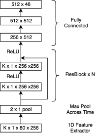
Fig. 1: CNN encoders, with filter size noted in each block. We have tuned $N$ and $K$ (time filter size) in our experiments.

2 Model Architecture

CTC is an approach to sequence labeling that uses a neural “encoder”, which maps from an input sequence of frame features $\textbf{x}=(x_{1},x_{2},\ldots,x_{T})$ to a sequence of hidden state vectors $h_{t}$, followed by a softmax to produce posterior probabilities of frame-level labels (referred to as “CTC labels”) $p(\pi_{t}|h_{t})$ for each label $\pi_{t}\in\mathcal{C}$. The posterior probability of a complete frame-level label sequence is taken to be the product of the frame posteriors:

$$p(\pi=\pi_{1},\pi_{2},\ldots,\pi_{T}|\mathbf{x})=\prod_{t}p(\pi_{t}|h_{t})$$ (1)

The CTC label set $\mathcal{C}$ consists of all of the possible true output labels (in our case, characters) plus a “blank” symbol $\phi$. Given a CTC label sequence, the hypothesized final label sequence is given by collapsing consecutive identical frame CTC labels and removing blanks. We use $B(\pi)$ to denote the collapsing function. All of the model parameters are learned jointly using the CTC loss function, which is the log posterior probability of the training label sequence $\textbf{z}=z_{1},z_{2}\ldots,z_{L}$ given input sequence $\mathbf{x}$,

$$\log p(\mathbf{z}|\mathbf{x}) = \log\sum_{\pi\in B^{-1}(\mathbf{z})}p(\pi|\mathbf{x})$$ (2)

$$= \log\sum_{\pi\in B^{-1}(\mathbf{z})}\prod_{t}p(\pi_{t}|h_{t})$$ (3)

Model parameters are learned using gradient descent; the gradient can be computed via a forward-backward technique [4].

2.1 Decoding

Our CTC models operate at a character level. We use the special blank symbol $\phi$ along with a vocabulary of 45 characters which appear in the raw SWB corpus (26 letters, 10 digits, space, &, ’, -, [laughter], [vocalized-noise], [noise], / and _). These transcriptions were inherited from a Switchboard Kaldi [15] setup without text normalization. We remove punctuation and noise tokens during post-processing. Decoding with CTC models can be done in a number of ways, depending on whether one uses a lexicon and/or a word- or character-level language model (LM) [16]. Here we focus on two simple cases, greedy decoding with no language model and beam-search decoding with an $n$-gram character LM.

To decode without a language model, we take the most likely CTC output label at each frame and collapse the resulting frame label sequence to the corresponding character sequence. We also consider decoding with an $n$-gram language model ($n=7,9$) using a beam search decoding procedure. We decode with the objective,

$$\mathbf{\hat{\pi}}=\operatorname*{arg\,max}_{\mathbf{\pi}\in\mathbf{\Pi}}~{}~{}p(\mathbf{k})^{\alpha}|\mathbf{k}|^{\beta}\prod_{t}p(\pi_{t}|h_{t})$$

where $\mathbf{k}=B(\mathbf{\pi})$, $|\mathbf{k}|$ denotes the length of $\mathbf{k}$, and $\alpha$, $\beta$ are tunable parameters. The final decoded output is $\mathbf{\hat{z}}=B(\mathbf{\hat{\pi}})$. Our beam-search method is the algorithm described in [5].

2.2 Encoders

We refer to the neural network that maps from the input x to state vectors h as an encoder. We consider both a typical recurrent LSTM encoder and various convolutional encoders. Our input vectors are 40 log mel frequency filterbank features (static) concatenated with their first-order derivatives (delta).

2.2.1 LSTMs

Our recurrent encoder is a multi-layer bi-directional LSTM with a dropout layer between consecutive layers (with dropout rate 0.1). We concatenate every two consecutive input vectors (as in [2]), which reduces the time resolution by a factor of two and speeds up both the forward and backward pass.

2.2.2 1-D CNNs

For our all-CNN encoders, we consider 1-D CNN structures that convolve across time only. Each of the input acoustic feature dimensions is treated as a separate input channel. The first layer is a convolution followed by max-pooling across time (with a stride size 2), followed by several convolutional layers, and ending with two 512-unit fully connected layers and a final projection layer. Each convolution has 256 channels. We add batch normalization after every convolution, and include residual connections between every pair of convolutional layers after the max-pool [17, 18]. A ReLU [19] non-linearity is used after every convolution, similar to the residual learning blocks in [17] (referred to as “ResBlocks (RBs)” in the rest of the paper). Fig. 1 portrays our architecture.

3 Experimental Setting

3.1 Data Setup

We use the Switchboard corpus (LDC97S62) [20], which contains roughly 300h of conversational telephone speech, as our training set. Following the Kaldi recipe [15], we reserve the first 4K utterances as a validation set. Since the training set has several repetitions of short utterances (like “uh-huh”), we remove duplicates beyond a count threshold of 300. The final training set has about 192K utterances. For evaluation, we use the HUB5 Eval2000 data set (LDC2002S09), consisting of two subsets: Switchboard (SWB), which is similar in style to the training set, and CallHome (CH), which contains conversations between friends and family. Our input filterbank features along with their deltas are normalized with per-speaker mean and variance normalization.

3.2 Training Setup

All models are trained on a single Titan X GPU with two supporting CPU threads, using TensorFlow r1.1 [21] and optimized using Adam [22] with a mini-batch size of 64 for LSTM (BasicLSTMCell) models and 32 for CNN models (unless otherwise mentioned). For the LSTM models, we use a learning rate of 0.001. For the CNN models, a smaller learning rate of 0.0002 was preferred. The learning rate is decayed by 5% whenever validation loss doesn’t decrease over two epochs. We report average training time per epoch for each model as both wall-clock hours ($t_{wc}$) and CPU-hours ($t_{cpu}$).

4 Results

4.1 LSTM Baseline

As a baseline, we train a 5-layer 320 hidden unit bi-directional recurrent neural network using LSTMs, similar to the architecture described in [16]. With a batch-size of 64, our LSTM needs $t_{wc}=3.3$ hours / epoch and $t_{cpu}=5.8$ hours / epoch. On a batch-size of 32, the LSTM takes $t_{wc}=8.7$ hours / epochs and $t_{cpu}=14.8$ hours / epoch.

Table 1: Development set WER for 1-D CNNs vs. number of layers. $b$ denotes batch-size. Each model is trained for 40 epochs with early stopping. $t_{wc}/t_{cpu}$ are hours / epoch.

Model	# Weights	WER %	$b$	$t_{wc}/t_{cpu}(h)$
5/320 LSTM	11.1M	28.54	64	3.3 / 5.8
10*1, 8 RBs	11.1M	36.71	32	0.9 / 2.2
10*1, 11 RBs	15.1M	32.67	32	1.0 / 2.5
10*1, 14 RBs	19.0M	30.92	32	1.1 / 2.8
10*1, 17 RBs	22.9M	29.82	32	1.5 / 3.5

4.2 1-D CNNs

We conduct experiments on 1-D CNNs investigating variance in performance and time / epoch with network depth and filter size. These are given in Table 1 and Table 2. We notice that for the same number of trainable parameters deeper networks with smaller filters seem to perform the best. We noticed that smaller-filter deeper architectures over-fit less when compared to larger-filter architectures with the same number of trainable parameters. For a fixed network depth, a mid-sized filter performed best. We present a graph of convergence vs wall-clock time in Fig. 2. As expected, the CNNs train faster than LSTMs, and significantly faster at the same batch-size. We also notice significant speed-ups during greedy decoding of the Eval2000 corpus, as shown in Table 3.

We show some of the learned filters in Fig. 3. These filters show that the network learns derivative-like filter patterns across different input channels. Our 1-D convolution structure with filter size $K$*1 can be viewed as similar to a 2-D convolution with filter size $K$*80, since the 1-D filters are learned jointly. We also note the strong relation between filter patterns learned in the static and delta regions.

Table 2: Development set WER for 1-D CNNs vs. filter size, each trained for 40 epochs with early stopping. The first two experiments vary filter size / depth at a constant number of trainable parameters (approximately for 15*1 filter). The third experiment varies filter size at a constant depth.

Model	# Weights	WER %	$t_{wc}/t_{cpu}(h)$
5*1, 16 RBs	11.1M	33.26	1.0 / 2.3
10*1, 8 RBs	11.1M	36.71	0.9 / 2.2
15*1, 5 RBs	10.5M	43.18	0.8 / 2.1
15*1, 6 RBs	12.4M	39.83	0.9 / 2.4
5*1, 28 RBs	19.0M	29.65	1.4 / 3.5
10*1, 14 RBs	19.0M	30.92	1.1 / 2.8
15*1, 9 RBs	18.3M	35.45	1.1 / 3.1
15*1, 10 RBs	20.3M	33.94	1.1 / 3.0
5*1, 14 RBs	9.8M	35.34	1.0 / 2.2
10*1, 14 RBs	19.0M	30.92	1.1 / 2.8
15*1, 14 RBs	28.1M	31.36	1.6 / 3.8

Table 3: Greedy decoding time on the Eval2000 corpus (4447 utterances). $b$ (batch-size) $=1$ is practical in real-time systems since it decodes one utterance at a time. $t_{wc}/t_{cpu}$ represent total decoding time in seconds averaged over three runs.

Model	# Weights	$b$	$t_{wc}$	/	$t_{cpu}$	$(s)$
5/320 LSTM	11.1M	1	1813	/	3667
5/320 LSTM	11.1M	32	87	/	180
5/320 LSTM	11.1M	64	44	/	92
5*1, 28 RBs, CNN	19.0M	1	115	/	135
5*1, 28 RBs, CNN	19.0M	32	17	/	18
5*1, 28 RBs, CNN	19.0M	64	15	/	16

4.3 Language Model Decoding

We evaluate our baseline LSTM and best performing CNN (5*1 filter with 28 RBs) on the Eval2000 corpus. We train each model to 50 epochs with early stopping on validation data. We augment our models with 7-gram and 9-gram character-level language models (LMs). These $n$-gram models were trained only on the SWB training corpus transcripts using SRILM [23]. For all experiments, a beam size of 200 was used. We choose $\alpha=0.6$ and $\beta=1.5$ after tuning on validation data. Our results are presented in Table 4. Notice that in the no LM results our CNNs are only 0.2% behind on the SWB part of Eval2000, but a larger 1.1% behind on CH. After LM decoding, the differences are more pronounced. This indicates that CNNs seem to over-fit more on the training data (which is similar to the SWB part of Eval2000) and show less improvement with the help of LMs.

Table 4: Final test set results on Eval2000.

Model	SWB	CH	EV
5/320 LSTM + no LM	27.7	47.5	37.6
5/320 LSTM + 7-g	20.0	38.5	29.3
5/320 LSTM + 9-g	19.7	38.2	29.0
5*1 28 RBs, CNN + no LM	27.9	48.6	38.3
5*1 28 RBs, CNN + 7-g	21.7	40.4	31.1
5*1 28 RBs, CNN + 9-g	21.3	40.0	30.7
Maas [5] + no LM	38.0	56.1	47.1
Maas [5] + 7-g	27.8	43.8	35.9
Maas [5] + RNN	21.4	40.2	30.8
Zenkel [16] + no LM	30.4	44.0	37.2
Zenkel [16] + RNN	18.6	31.6	25.1
Zweig [8] + no LM	25.9	38.8	-
Zweig [8] + $n$-g	19.8	32.1	-

5 Conclusions

We take a further step towards making all-convolutional CTC architectures practical for speech recognition. In particular we have explored 1-D convolutions with CTC, which are particularly time-efficient. Our CNN-based CTC models are still slightly behind LSTMs in performance, but train and decode significantly faster. Further work in this space could include additional model variants and regularizers, as well as studying the relative merits of all-convolutional models in larger systems operating at the word level, where the efficiency advantages are expected to be even more important. In addition, CNN-based speech recognition has also been explored in the context of different training and decoding algorithms, such as the auto segmentation criterion [24]. It would be interesting to conduct a broader study considering the interaction of CNNs with different training and decoding approaches.

6 Acknowledgements

We are grateful to Shubham Toshniwal for help with the data and baselines, and to Florian Metze for useful comments.

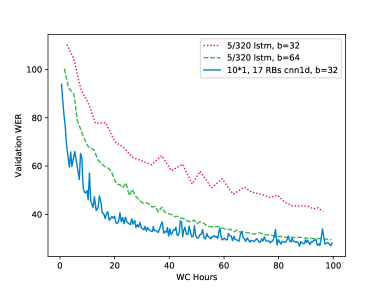
Fig. 2: Comparison of convergence vs. wall-clock time. 5/320 denotes the 5-layer 320-unit LSTM, $b$ = batch size.

Fig. 3: Visualization of the filters in the first layer for the 10*1, 17 RBs 1-D CNN. For each filter, the horizontal axis represents time and the vertical axis represents the 80 input channels (40 static + 40 delta, separated by the checkerboard pattern). The $6^{th}$ and $7^{th}$ images are a $\max$ and $\min$ over all 256 output channels.

References

- [1] Ilya Sutskever, Oriol Vinyals, and Quoc V Le, “Sequence to sequence learning with neural networks,” in Advances in NIPS, 2014.
- [2] William Chan, Navdeep Jaitly, Quoc Le, and Oriol Vinyals, “Listen, attend and spell: A neural network for large vocabulary conversational speech recognition,” in ICASSP, 2016.
- [3] Rohit Prabhavalkar, Kanishka Rao, Tara N Sainath, Bo Li, Leif Johnson, and Navdeep Jaitly, “A comparison of sequence-to-sequence models for speech recognition,” Interspeech, 2017.
- [4] Alex Graves, Santiago Fernández, Faustino Gomez, and Jürgen Schmidhuber, “Connectionist temporal classification: labelling unsegmented sequence data with recurrent neural networks,” in Proceedings of ICML, 2006.
- [5] Andrew L Maas, Ziang Xie, Dan Jurafsky, and Andrew Y Ng, “Lexicon-free conversational speech recognition with neural networks,” in HLT-NAACL, 2015.
- [6] Dario Amodei, Sundaram Ananthanarayanan, Rishita Anubhai, Jingliang Bai, Eric Battenberg, Carl Case, Jared Casper, Bryan Catanzaro, Qiang Cheng, Guoliang Chen, et al., “Deep Speech 2: End-to-end speech recognition in English and Mandarin,” in Proceedings of ICML, 2016.
- [7] Yajie Miao, Mohammad Gowayyed, and Florian Metze, “EESEN: End-to-end speech recognition using deep RNN models and WFST-based decoding,” in ASRU, 2015.
- [8] Geoffrey Zweig, Chengzhu Yu, Jasha Droppo, and Andreas Stolcke, “Advances in all-neural speech recognition,” in ICASSP, 2017.
- [9] Ying Zhang, Mohammad Pezeshki, Philémon Brakel, Saizheng Zhang, César Laurent, Yoshua Bengio, and Aaron C. Courville, “Towards end-to-end speech recognition with deep convolutional neural networks,” in Interspeech, 2016.
- [10] Yisen Wang, Xuejiao Deng, Songbai Pu, and Zhiheng Huang, “Residual convolutional CTC networks for automatic speech recognition,” CoRR, vol. abs/1702.07793, 2017.
- [11] Alexander Waibel, Toshiyuki Hanazawa, Geoffrey Hinton, Kiyohiro Shikano, and Kevin J Lang, “Phoneme recognition using time-delay neural networks,” in Readings in speech recognition. Elsevier, 1990.
- [12] Vijayaditya Peddinti, Daniel Povey, and Sanjeev Khudanpur, “A time delay neural network architecture for efficient modeling of long temporal contexts,” in Interspeech, 2015.
- [13] Kartik Audhkhasi, Bhuvana Ramabhadran, George Saon, Michael Picheny, and David Nahamoo, “Direct acoustics-to-word models for English conversational speech recognition,” in Interspeech, 2017.
- [14] Hagen Soltau, Hank Liao, and Hasim Sak, “Neural speech recognizer: Acoustic-to-word LSTM model for large vocabulary speech recognition,” in Interspeech, 2017.
- [15] Daniel Povey, Arnab Ghoshal, Gilles Boulianne, Lukas Burget, Ondrej Glembek, Nagendra Goel, Mirko Hannemann, Petr Motlicek, Yanmin Qian, Petr Schwarz, et al., “The Kaldi speech recognition toolkit,” in ASRU, 2011.
- [16] Thomas Zenkel, Ramon Sanabria, Florian Metze, Jan Niehues, Matthias Sperber, Sebastian Stüker, and Alex Waibel, “Comparison of decoding strategies for CTC acoustic models,” in Interspeech, 2017.
- [17] Kaiming He, Xiangyu Zhang, Shaoqing Ren, and Jian Sun, “Deep residual learning for image recognition,” in CVPR, 2016.
- [18] Sergey Ioffe and Christian Szegedy, “Batch normalization: Accelerating deep network training by reducing internal covariate shift,” in Proceedings of ICML, 2015.
- [19] Vinod Nair and Geoffrey E Hinton, “Rectified linear units improve restricted Boltzmann machines,” in Proceedings of ICML, 2010.
- [20] John J Godfrey, Edward C Holliman, and Jane McDaniel, “SWITCHBOARD: Telephone speech corpus for research and development,” in ICASSP, 1992.
- [21] Martín Abadi, Ashish Agarwal, Paul Barham, Eugene Brevdo, Zhifeng Chen, Craig Citro, Greg Corrado, Andy Davis, Jeffrey Dean, et al., “Tensorflow: Large-scale machine learning on heterogeneous distributed systems,” 2015.
- [22] Diederik Kingma and Jimmy Ba, “Adam: A method for stochastic optimization,” in ICLR, 2015.
- [23] Andreas Stolcke et al., “SRILM-an extensible language modeling toolkit,” in Interspeech, 2002.
- [24] Ronan Collobert, Christian Puhrsch, and Gabriel Synnaeve, “Wav2Letter: an end-to-end convnet-based speech recognition system,” CoRR, vol. abs/1609.03193, 2016.