Minimax Rates and Efficient Algorithms for Noisy Sorting

Abstract

There has been a recent surge of interest in studying permutation-based models for ranking from pairwise comparison data. Despite being structurally richer and more robust than parametric ranking models, permutation-based models are less well understood statistically and generally lack efficient learning algorithms. In this work, we study a prototype of permutation-based ranking models, namely, the noisy sorting model. We establish the optimal rates of learning the model under two sampling procedures. Furthermore, we provide a fast algorithm to achieve near-optimal rates if the observations are sampled independently. Along the way, we discover properties of the symmetric group which are of theoretical interest.

Keywords: Noisy Sorting, Pairwise Comparisons, Ranking, Permutations, Minimax Estimation

1 Introduction

Pairwise comparison data is frequently observed in various domains, including recommender systems, website ranking, voting and social choice (see, e.g. Baltrunas et al., 2010; Dwork et al., 2001; Liu, 2009; Young, 1988; Caplin and Nalebuff, 1991). For these applications, it is of significant interest to produce a suitable ranking of the items by aggregating the outcomes of pairwise comparisons. The general problem of interest can be stated as follows. Suppose there are $n$ items to be compared and an underlying matrix $P$ of probability parameters, each entry $P_{i,j}$ of which represents the probability that item $i$ beats item $j$ if they are compared. Hence we have $P_{j,i}=1-P_{i,j}$ and the event that item $i$ beats item $j$ in a comparison can be viewed as a Bernoulli random variable with probability $P_{i,j}$. Observing the outcomes of $N$ independent pairwise comparisons, we aim to estimate the absolute ranking of the items.

For the sake of consistency, one needs of course to impose some structure on the matrix $P=\{P_{i,j}\}_{1\leq i,j\leq n}$. These structural assumptions are traditionally split between parametric and nonparametric ones. Classical parametric models include the Bradley-Terry-Luce model (Bradley and Terry, 1952; Luce, 1959) and the Thurstone model (Thurstone, 1927). These models can be recast as log-linear models, which enables the use of the statistical and computational machinery of maximum likelihood estimation in generalized linear models (Hunter, 2004; Negahban et al., 2012; Rajkumar and Agarwal, 2014; Hajek et al., 2014; Shah et al., 2015; Negahban et al., 2016, 2017).

To allow richer structures on $P$ beyond the scope of parametric models, permutation-based models such as the noisy sorting model (Braverman and Mossel, 2008, 2009) and the strong stochastic transitivity (SST) model (Chatterjee, 2015; Shah et al., 2017a) have recently become more prevalent. These models only require shape constraints on the matrix $P$ and are typically called nonparametric. In these models, the underlying ranking of items is determined by an unknown permutation $\pi^{*}$, and, additionally, the comparison probabilities are assumed to have a bi-isotonic structure when the items are aligned according to $\pi^{*}$. While permutation-based models provide ordering structures that are not captured by parametric models (Agarwal, 2016; Shah et al., 2017a), they introduce both statistical and computational barriers for estimation of the underlying ranking. These barriers are mainly due to the complexity of the discrete set of permutations. On the one hand, the complexity of the set of permutations is not well understood (see the discussion following Theorem 8 in Collier and Dalalyan, 2016), which leads to logarithmic gaps in the current statistical bounds for permutation-based models. On the other hand, it is computationally challenging to optimize over the set of permutations, so current algorithms either sacrifice nontrivial statistical performance or have impractical time complexity. In this work, we aim to address both questions for the noisy sorting model.

In practice, it is unlikely that all the items are compared to each other. To account for this limitation, a widely used scheme consists in assuming that that each pairwise comparison is observed with probability $p\in(0,1]$ (see, e.g. Chatterjee, 2015; Shah et al., 2017a). In addition to this model of missing comparisons, we study the model where $N$ pairwise comparisons are sampled uniformly at random from the $\binom{n}{2}$ pairs, with replacement and independent of each other. It turns out that sampling with and without replacement yields the same rate of estimation up to a constant when the expected numbers of observations coincide.

Our contributions.

We focus on the noisy sorting model with partial observations, under which a stronger item wins a comparison against a weaker item with probability at least $\frac{1}{2}+\lambda$ where $\lambda\in(0,\frac{1}{2})$. For sampling both with and without replacement, we establish the minimax rate of learning the underlying permutation. In particular, the rate does not involve a logarithmic term, and we explain this phenomenon through a careful analysis of the metric entropy of the set of permutations equipped with the Kendall tau distance, which is of independent theoretical interest.

Moreover, we propose a multistage sorting algorithm that has time complexity $\tilde{O}(n^{2})$. For the sampling with replacement model, we prove a theoretical guarantee on the performance of the multistage sorting algorithm, which differs from the minimax rate by only a polylogarithmic factor. In addition, the algorithm is demonstrated to perform similarly for both sampling models using simulated examples.

Related work.

The noisy sorting model was proposed by Braverman and Mossel (2008). In the original paper, the optimal rate of estimation achieved by the maximum likelihood estimator (MLE) is established, and an algorithm with time complexity $O(n^{C})$ is shown to find the MLE with high probability in the case of full observations, where $C=C(\lambda)$ is a large unknown constant. Moreover, their algorithm does not have a polynomial running time if only $o(n^{2})$ random pairwise comparisons are observed. Our work generalizes the optimal rate to the partial observation settings by studying a variant of the MLE for the upper bound. In the model of sampling with replacement, our fast multistage sorting algorithm provably achieves near-optimal rate of estimation. Since finding the MLE for the noisy sorting model is an instance of the NP-hard feedback arc set problem (Alon, 2006; Kenyon-Mathieu and Schudy, 2007; Ailon et al., 2008; Braverman and Mossel, 2008), our results indicate that, despite the NP-hardness of the worst-case problem, it is still possible to achieve (near-)optimal rates for the average-case statistical setting in polynomial time.

The SST model generalizes the noisy sorting model, and minimax rates in the SST model have been studied by Shah et al. (2017a). However, the upper bound specialized to noisy sorting contains an extra logarithmic factor, which this work shows to be unnecessary. Moreover, the lower bound there is based on noisy sorting models with $\lambda$ shrinking to zero as $n\to\infty$, while we establish a matching lower bound at any fixed $\lambda$. In addition, algorithms of Wauthier et al. (2013); Shah et al. (2017a); Chatterjee and Mukherjee (2016) are all statistically suboptimal for the noisy sorting model. This is partially addressed by our multistage sorting algorithm as discussed above.

In fact, both with- and without-replacement sampling models discussed in this paper are restrictive for applications where the set of observed comparisons is subject to certain structural constraints (Hajek et al., 2014; Shah et al., 2015; Negahban et al., 2017; Pananjady et al., 2017a). Obtaining sharper rates of estimation for these more complex sampling models is of significant interest but is beyond the scope of the current work.

Finally, we mention a few other lines of related work. Besides permutation-based models, low-rank structures have also been proposed by Rajkumar and Agarwal (2016) to generalize classical parametric models. Moreover, there is an extensive literature on active ranking from pairwise comparisons (see, e.g., Jamieson and Nowak, 2011; Heckel et al., 2016; Agarwal et al., 2017, and references therein), where the pairs to be compared are chosen actively and in a sequential fashion by the learner. The sequential nature of the models greatly reduces sample complexity, so we do not compare our results for passive observations to the literature on active learning. However, it is interesting to note that our multistage sorting algorithm is reminiscent of active algorithms, because it uses different batches of samples for different stages. Thus active learning algorithms could potentially be useful even for passive sampling models.

Organization.

The noisy sorting model together with the two sampling models is formalized in Section 2. In Section 3, we present our main results, the minimax rate of estimation for the latent permutation and the near-optimal rate achieved by an efficient multistage sorting algorithm. To complement our theoretical findings, we inspect the empirical performance of the multistage sorting algorithm on numerical examples in Section 4. Section 5 is devoted to the study of the set of permutations equipped with the Kendall tau distance. Proofs of the main results are provided in Section 6. We discuss directions for future research in Section 7.

Notation.

For a positive integer $n$, let $[n]=\{1,\ldots,n\}$. For a finite set $S$, we denote its cardinality by $|S|$. Given $a,b\in\mathbbm{R}$, let $a\wedge b=\min(a,b)$ and $a\vee b=\max(a,b)$. We use $C$ and $c$, possibly with subscripts, to denote universal positive constants that may change at each appearance. For two sequences $\{u_{n}\}_{n=1}^{\infty}$ and $\{v_{n}\}_{n=1}^{\infty}$, we write $u_{n}\lesssim v_{n}$ if there exists a universal constant $C>0$ such that $u_{n}\leq Cv_{n}$ for all $n$. We define the relation $u_{n}\gtrsim v_{n}$ analogously, and write $u_{n}\asymp v_{n}$ if both $u_{n}\lesssim v_{n}$ and $u_{n}\gtrsim v_{n}$ hold. Let $\mathfrak{S}_{n}$ denote the symmetric group on $[n]$, i.e., the set of permutations $\pi:[n]\to[n]$.

2 Problem formulation

The noisy sorting model can be formulated as follows. Fix an unknown permutation $\pi^{*}\in\mathfrak{S}_{n}$ which determines the underlying order of $n$ items. More precisely, $\pi^{*}$ orders the items from the weakest to the strongest, so that item $i$ is the $\pi^{*}(i)$-th weakest among the $n$ items. For a fixed $\lambda\in(0,1/2)$, we define a class of matrices

$$\mathcal{M}_{n}(\lambda)=\Big{\{}M\in[0,1]^{n\times n}\,:\,\,M_{i,i}=\frac{1}{2}\,,\ M_{i,j}\geq\frac{1}{2}+\lambda\ \text{if}\ i>j\,,\ M_{i,j}\leq\frac{1}{2}-\lambda\ \text{if}\ i<j\Big{\}}\,,$$

where $\mathbf{1}_{n}$ is the $n$-dimensional all-ones vector. In addition, we define a special matrix $M^{*}_{n}(\lambda)\in\mathcal{M}_{n}(\lambda)$ by

$$[M^{*}_{n}(\lambda)]_{i,j}=\begin{cases}1/2+\lambda&\text{ if }i>j\,,\\ 1/2-\lambda&\text{ if }i<j\,,\\ 1/2&\text{ if }i=j\,.\end{cases}$$

Note that $M^{*}_{n}(\lambda)$ satisfies strong stochastic transitivity but other matrices $M\in\mathcal{M}_{n}(\lambda)$ may not. Though this observation plays a crucial role in the design of efficient algorithms, our statistical results hold for general matrices in $\mathcal{M}_{n}(\lambda)$.

To model pairwise comparisons, fix $M\in\mathcal{M}_{n}(\lambda)$ and let $M_{\pi^{*}(i),\pi^{*}(j)}$ denote the probability that items $i$ beats item $j$ when they are compared, so that a stronger item beats a weaker item with probability at least $\frac{1}{2}+\lambda$. As a result, $\lambda$ captures the signal-to-noise ratio of our problem and our minimax results explicitly capture the dependence in this key parameter.

2.1 Sampling models

In the noisy sorting model, suppose that for each (unordered) pair $(i,j)$ with $i\neq j$, we observe the outcomes of $N_{i,j}(=N_{j,i})$ comparisons between them, and item $i$ wins a comparison against item $j$ with probability $M_{\pi^{*}(i),\pi^{*}(j)}$ independently. The set $\{N_{i,j}\}_{i<j}$ of $\binom{n}{2}$ nonnegative integers is determined by certain sampling models described below. We allow $N_{i,j}$ to be zero, which means that $i$ and $j$ are not compared. We collect sufficient statistics into a matrix $A\in\mathbbm{R}^{n\times n}$ consisting of outcomes of pairwise comparisons, by defining $A_{i,j}$ to be the number of times item $i$ beats item $j$ among the $N_{i,j}$ comparisons between $i$ and $j$. In particular, we have $A_{i,j}+A_{j,i}=N_{i,j}=N_{j,i}$ for $i\neq j$ and $A_{i,i}=0$. Our goal is to aggregate the results of pairwise comparisons to estimate $\pi^{*}$, the underlying order of items.

In the full observation setup of Braverman and Mossel (2008), we have $N_{i,j}=1$ for each pair $(i,j)$ and the total number of observations is $N:\,=\sum_{i<j}N_{i,j}=\binom{n}{2}$. Instead, we are interested here in the regime where the total number of observations $N$ is much smaller than $\binom{n}{2}$. We study the following two sampling models in this work:

1. Sampling without replacement. In this sampling model, instead of observing all the pairwise comparisons, we observe each pair with probability $p\in(0,1]$ independently. Hence each $N_{i,j}\sim\mathsf{Ber}(p)$ is a Bernoulli random variable with parameter $p$, and in expectation we have $p\binom{n}{2}$ observations in total.

2. Sampling with replacement. We observe $N$ pairwise comparisons between the items, sampled uniformly and independently with replacement from the $\binom{n}{2}$ pairs.

In the sequel, we study the noisy sorting model with either of the above two sampling models. In particular, the minimax rates of estimating $\pi^{*}$ coincide for the two sampling models if $p\binom{n}{2}\asymp N$, i.e., if the expected number of observations are of the same order.

2.2 Measures of performance

Having discussed the sampling and comparison models, we turn to the distance used to measure the difference between the underlying permutation $\pi^{*}$ and an estimated permutation $\hat{\pi}$. Among various distances defined on the symmetric group, we consider primarily the Kendall tau distance, i.e., the number of inversions (or discordant pairs) between permutations, defined as

$$d_{\mathsf{KT}}(\pi,\sigma)=\sum_{(i,j):\sigma(i)<\sigma(j)}\mathbbm{1}\big{(}\pi(i)>\pi(j)\big{)}$$

for $\pi,\sigma\in\mathfrak{S}_{n}$. Note that $0\leq d_{\mathsf{KT}}(\pi,\sigma)\leq\binom{n}{2}$. The Kendall tau distance between two permutations is a natural metric on $\mathfrak{S}_{n}$, and it is equal to the minimum number of adjacent transpositions required to change from one permutation to another (Knuth, 1998). A closely related distance on $\mathfrak{S}_{n}$ is the $\ell_{1}$-distance, also known as Spearman’s footrule, defined as

$$\|\pi-\sigma\|_{1}=\sum_{i=1}^{n}|\pi(i)-\sigma(i)|$$

for $\pi,\sigma\in\mathfrak{S}_{n}$. It is well known (Diaconis and Graham, 1977) that

$$d_{\mathsf{KT}}(\pi,\sigma)\leq\|\pi-\sigma\|_{1}\leq 2d_{\mathsf{KT}}(\pi,\sigma)\,.$$ (2.1)

Hence the rates of estimation in the two distances coincide. Another distance on $\mathfrak{S}_{n}$ we use is the $\ell_{\infty}$-distance, defined as

$$\|\pi-\sigma\|_{\infty}=\max_{i\in[n]}\,|\pi(i)-\sigma(i)|\,.$$

Note that unlike existing literature on ranking from pairwise comparisons where metrics on the probability parameters are studied, we employ here distances that measure how far an item is from its true ranking.

3 Main results

In this section, we state our main results. Specifically, we establish the minimax rates of estimating $\pi^{*}$ in the Kendall tau distance (and thus in $\ell_{1}$ distance) for noisy sorting under both sampling models ($O_{1}$) and ($O_{2}$). The minimax estimator that we propose is intractable in general and we complement our results with an efficient estimator of $\pi^{*}$ which achieves near-optimal rates in both the Kendall tau and the $\ell_{\infty}$-distance, under the sampling model ($O_{2}$).

3.1 Minimax rates of noisy sorting

Under the noisy sorting model with latent permutation $\pi^{*}\in\mathfrak{S}_{n}$ and matrix of probabilities $M\in\mathcal{M}_{n}(\lambda)$, we determine the minimax rate of estimating $\pi^{*}$ in the following theorem. Let $\mathbbm{E}_{\pi^{*},M}$ denote the expectation with respect to the probability distribution of the observations in the noisy sorting model with underlying permutation $\pi^{*}\in\mathfrak{S}_{n}$ and matrix of probabilities $M\in\mathcal{M}_{n}(\lambda)$, in either sampling model.

Theorem 1

Fix $\lambda\in(0,\frac{1}{2}-c]$ where $c$ is a universal positive constant. It holds that

$$\min_{\tilde{\pi}}\max_{\begin{subarray}{c}\pi^{*}\in\mathfrak{S}_{n}\\ M\in\mathcal{M}_{n}(\lambda)\end{subarray}}\mathbbm{E}_{\pi^{*},M}[d_{\mathsf{KT}}(\tilde{\pi},\pi^{*})]\asymp\left\{\begin{array}[]{ll}\displaystyle\frac{n}{p\lambda^{2}}\land n^{2}\,,&\text{in sampling model \ref{model:1}}\,,\\ \displaystyle\frac{n^{3}}{N\lambda^{2}}\land n^{2}\,,&\text{in sampling model \ref{model:2}}\,,\end{array}\right.$$

where the minimum is taken minimized over all permutation estimators $\tilde{\pi}\in\mathfrak{S}_{n}$ that are measurable with respect to the observations.

The theorem establishes the minimax rates for noisy sorting, including the case of partial observations and weak signals. The upper bounds in fact hold with high probability as shown in Theorem 7. If the expected numbers of observations in the two sampling models ($O_{1}$) and ($O_{2}$) are of the same order, i.e., $p\binom{n}{2}\asymp N$, then the two rates coincide. In this sense, the two sampling models are statistically equivalent. In sampling model ($O_{1}$), if $p=1$ and $\lambda$ is larger than a constant, then the rate of order $n$ recovers the upper bound proved by Braverman and Mossel (2008).

Note in particular the absence of logarithmic factor in the rates. Naively bounding the metric entropy of $\mathfrak{S}_{n}$ by $\log|\mathfrak{S}_{n}|\simeq n\log n$ actually yields a superfluous logarithmic term in the upper bound. To avoid it, we study the doubling dimension of $\mathfrak{S}_{n}$; see the discussion after Proposition 3. Closing this logarithmic gap for other problems involving latent permutations (Collier and Dalalyan, 2016; Flammarion et al., 2016; Shah et al., 2017a; Pananjady et al., 2017b) remains an open question.

The technical assumption $\lambda\leq 1/2-c$ in Theorem 1 is very mild, because we are interested in the “noisy” sorting model (meaning that the pairwise comparisons are noisy, or equivalently that $\lambda$ is not close to $\frac{1}{2}$). In fact the requirement that $\lambda$ be bounded away from $\frac{1}{2}$ can be lifted, in which case we establish upper and lower bounds that match up to a logarithmic factor of order $\log(1/\Delta)$, where $\Delta=1/2-\lambda$ (see Section 6).

Finally, we note that the proof of Theorem 1 holds even in the so-called semi-random setting (Blum and Spencer, 1995; Makarychev et al., 2013), in which observations are generated by one of the random procedures described above, but a “helpful” adversary is allowed to reverse the outcome of any comparison in which a weaker item beat a stronger item. Though these reversals appear benign at first glance, the presence of such an adversary can in fact worsen statistical rates of estimation in more brittle models such as stochastic block models and the related broadcast tree model (Moitra et al., 2016). Our results indicate that no such degradation occurs for the rates of estimation in the noisy sorting problem.

3.2 Efficient multistage sorting

The minimax upper bound in Theorem 1 is established using a computationally prohibitive estimator, so we now introduce an efficient estimator of the underlying permutation that can be computed in time $\tilde{O}(n^{2})$. In this section, we prove theoretical guarantees for this estimator under the noisy sorting model with probability matrix $M=M^{*}_{n}(\lambda)$ and observations sampled with replacement according to ($O_{2}$) when $\lambda$ is bounded away from zero by a universal constant. No polynomial-time algorithm was previously known to achieve near-optimal rates even in this simplified setting when $o(n^{2})$ pairwise comparisons are observed.

Since we aim to prove guarantees up to constants, we may assume that we have $2N$ pairwise comparisons, and split them into two independent samples, each containing $N$ pairwise comparisons. The first sample is used to estimate the parameter $\lambda$ and the second one is used to estimate the permutation $\pi^{*}$.

First, we introduce a fairly simple estimator $\hat{\lambda}$ of $\lambda$ that can be described informally as follows: first sort in increasing order the items according to the number of wins. Then for any pair $(i,j)$ for which item $i$ is ranked $n/2$ positions higher than item $j$, it is very likely that item $i$ is stronger than item $j$ so that it beats item $j$ with probability $\frac{1}{2}+\lambda$. We then average the $\mathsf{Ber}(\frac{1}{2}+\lambda)$ variables over all such pairs to obtain an estimator $\hat{\lambda}$ of $\lambda$. More formally, we further split the first sample into two subsamples, each containing $N/2$ pairwise comparisons. Denote by $A_{i,j}^{\prime}$ and $A_{i,j}^{\prime\prime}$ the number of wins item $i$ has against item $j$ in the first and second subsample, respectively. The estimator $\hat{\lambda}$ is given by the following procedure:

1. For each $i\in[n]$, associate with item $i$ a score $S_{i}=\sum_{j=1}^{n}A_{i,j}^{\prime}$.

2. Construct a permutation $\tilde{\pi}$ by sorting the scores $S_{i}$ in increasing order, i.e., $\tilde{\pi}$ is chosen so that $\tilde{\pi}(i)<\tilde{\pi}(j)$ if $S_{i}\leq S_{j}$, with ties broken arbitrarily.

3. Define $\displaystyle\hat{\lambda}=\frac{2}{N}\binom{n}{2}\binom{n/2}{2}^{-1}\sum_{\tilde{\pi}(i)-\tilde{\pi}(j)>\frac{n}{2}}A_{i,j}^{\prime\prime}-\frac{1}{2}.$

Given the estimator $\hat{\lambda}$, we now describe a multistage procedure to estimate the permutation $\pi^{*}$. To recover the underlying order of items, it is equivalent to estimate the row sums $\sum_{j=1}^{n}M_{\pi^{*}(i),\pi^{*}(j)}$ which we call scores of the items, because the scores are increasing linearly if the items are placed in order. Initially, for each $i\in[n]$, we estimate the score of item $i$ by the number of wins item $i$ has. If item $i$ has a much higher score than item $j$ in the first stage, then we are confident that item $i$ is stronger than item $j$. Hence in the second stage, we can estimate $M_{\pi^{*}(i),\pi^{*}(j)}$ by $\frac{1}{2}+\hat{\lambda}$, which is very close to the truth. For those pairs that we are not certain about, $M_{\pi^{*}(i),\pi^{*}(j)}$ is still estimated by its empirical version. The variance of each score is thus greatly reduced in the second stage, thereby yielding a more accurate order of the items. Then we iterate this process to obtain finer and finer estimates of the scores and the underlying order.

To present the Multistage Sorting (MS) algorithm formally, let us fix a positive integer $T$ which is the number of stages of the algorithm. We further split the second sample into $T$ subsamples each containing $N/T$ pairwise comparisons. Similar to the data matrix $A$ for the full sample, for $t\in[T]$ we define a matrix $A^{(t)}\in\mathbbm{R}^{n\times n}$ by setting $A^{(t)}_{i,j}$ to be the number of wins item $i$ has against item $j$ in the $t$-th sample. The MS algorithm proceeds as follows:

1. For each $i\in[n]$, define $I^{(0)}(i)=[n]$, $I^{(0)}_{-}(i)=\varnothing$ and $I^{(0)}_{+}(i)=\varnothing$.

2. At the $t$-th stage where $t\in[T]$, compute the score $S^{(t)}_{i}$ of item $i$:

   $$S^{(t)}_{i}=\frac{Tn(n-1)}{2N}\sum_{j\in I^{(t-1)}(i)}A^{(t)}_{i,j}+\sum_{j\in I^{(t-1)}_{-}(i)}\big{(}\frac{1}{2}+\hat{\lambda}\big{)}+\sum_{j\in I^{(t-1)}_{+}(i)}\big{(}\frac{1}{2}-\hat{\lambda}\big{)}\,.$$

3. Let $C_{0}$ and $C_{1}$ be sufficiently large universal constants. If it holds that

   $$|I^{(t-1)}(i)|\geq C_{1}n^{2}\frac{T}{N}\log(nT)\,,$$ (3.1)

   then we set the threshold

   $$\tau_{i}^{(t)}=(10+2C_{0})n\sqrt{|I^{(t-1)}(i)|TN^{-1}\log(nT)}\,,$$

   and define the sets

   $$I^{(t)}_{-}(i) =\{j\in[n]:S^{(t)}_{j}-S^{(t)}_{i}<-\tau_{i}^{(t)}\},$$

   $$I^{(t)}_{+}(i) =\{j\in[n]:S^{(t)}_{j}-S^{(t)}_{i}>\tau_{i}^{(t)}\},\text{ and}$$

   $$I^{(t)}(i) =[n]\setminus\big{(}I^{(t)}_{-}(i)\cup I^{(t)}_{+}(i)\big{)}\,.$$

   If (3.1) does not hold, then we define $I^{(t)}(i)=I^{(t-1)}(i)$, $I_{-}^{(t)}(i)=I_{-}^{(t-1)}(i)$ and $I_{+}^{(t)}(i)=I_{+}^{(t-1)}(i)$. Note that $I^{(t)}(i)$ denotes the set of items $j$ whose ranking relative to $i$ has not been determined by the algorithm at stage $t$.

4. After repeating Step 2 and 3 for $t=1,\dots,T$, output a permutation $\hat{\pi}^{\scriptscriptstyle{\sf MS}}$ by sorting the scores $S^{(T)}_{i}$ in increasing order, i.e., $\hat{\pi}^{\scriptscriptstyle{\sf MS}}$ is chosen so that $\hat{\pi}^{\scriptscriptstyle{\sf MS}}(i)<\hat{\pi}^{\scriptscriptstyle{\sf MS}}(j)$ if $S^{(T)}_{i}\leq S^{(T)}_{j}$ with ties broken arbitrarily.

It is clear that the time complexity of each stage of the algorithm is $O(n^{2})$. Take $T=\lfloor\log\log n\rfloor$ so that the overall time complexity of the MS algorithm is only $O(n^{2}\log\log n)$. Our main result in this section is the following guarantee on the performance of the estimator $\hat{\pi}^{\scriptscriptstyle{\sf MS}}$ given by the MS algorithm.

Theorem 2

Suppose that $N\geq Cn\log n$ for a sufficiently large constant $C>0$ and that $M=M^{*}_{n}(\lambda)$ where $\lambda\in[c,\frac{1}{2})$ for a constant $c>0$. Then, under the noisy sorting model with sampling model ($O_{2}$), the following holds. With probability at least $1-n^{-7}$, the MS algorithm with $T=\lfloor\log\log n\rfloor$ stages outputs an estimator $\hat{\pi}^{\scriptscriptstyle{\sf MS}}$ that satisfies

$$\|\hat{\pi}^{\scriptscriptstyle{\sf MS}}-\pi^{*}\|_{\infty}\lesssim\frac{n^{2}}{N}(\log n)\log\log n$$

and

$$d_{\mathsf{KT}}(\hat{\pi}^{\scriptscriptstyle{\sf MS}},\pi^{*})\lesssim\frac{n^{3}}{N}(\log n)\log\log n\,.$$

Note that the second statement follows from the first one together with (2.1). Indeed, we have

$$d_{\mathsf{KT}}(\hat{\pi}^{\scriptscriptstyle{\sf MS}},\pi^{*})\leq\|\hat{\pi}^{\scriptscriptstyle{\sf MS}}-\pi^{*}\|_{1}\leq n\|\hat{\pi}^{\scriptscriptstyle{\sf MS}}-\pi^{*}\|_{\infty}\lesssim\frac{n^{3}}{N}(\log n)\log\log n\,,$$

which is optimal up to a polylogarithmic factor in the regime where $\lambda$ is bounded away from $0$ according to Theorem 1 (and Theorem 8). Therefore, the MS algorithm achieves significant computational efficiency while sacrificing little in terms of statistical performance. On the downside, it is limited to the noisy sorting model where $M=M_{n}^{*}(\lambda)$—this assumption is necessary to exploit strong stochastic transitivity—and our analysis does not account for the dependence in $\lambda$.

Furthermore, although we only consider model ($O_{2}$) of sampling with replacement in this section, the MS algorithm can be easily modified to handle model ($O_{1}$) of sampling without replacement. It is much more challenging to prove analogous theoretical guarantees in this case, because we cannot split the observations into independent samples. In Section 4, however, we provide empirical evidence showing that the MS estimator has very similar performance for the two sampling models.

Our algorithm bears comparison with the algorithm proposed by Braverman and Mossel (2008). Their algorithm—which works in the full observation case $N=\binom{n}{2}$—achieves the statistically optimal rate in time $O(n^{C})$, where $C$ is a large positive constant depending on $\lambda$. Though our algorithm’s statistical performance falls short of the optimal rate by a polylogarithmic factor, it runs in time $O(n^{2}\log\log n)$ and works in the partial observation setting as long as $N\gtrsim n\log n$. Note by way of comparison that Theorem 8 indicates that no procedure achieves nontrivial recovery unless $N\gg n$.

4 Simulations

To support our theoretical findings in Section 3.2, we implement the MS algorithm on synthetic instances generated from the noisy sorting model. For simplicity, we take $\lambda=0.25$ and set $\hat{\lambda}=\lambda$ in the algorithm. Theorem 2 predicts a scaling $n^{3}N^{-1}(\log n)\log\log n$ of the estimation error in the Kendall tau distance for model ($O_{2}$) of sampling with replacement, where $n$ is the number of items and $N$ is the number of pairwise comparisons. This rate is optimal up to a polylogarithmic factor according to Theorem 8.

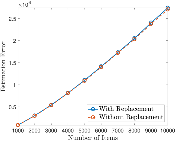
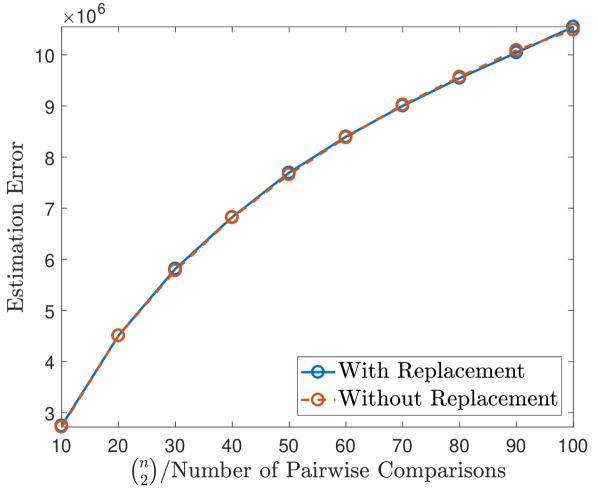
Figure 1: Estimation errors $d_{\mathsf{KT}}(\hat{\pi}^{\scriptscriptstyle{\sf MS}},\pi^{*})$ for the observations sampled with and without replacement. Left: $N=p\binom{n}{2}=0.1\binom{n}{2}$ and $n$ ranging from $1,000$ to $10,000$; Right: $n=10,000$ and $N=p\binom{n}{2}$ ranging from $0.1\binom{n}{2}$ to $0.01\binom{n}{2}$.

In Figure 1, we plot estimation errors $d_{\mathsf{KT}}(\hat{\pi}^{\scriptscriptstyle{\sf MS}},\pi^{*})$ averaged over $10$ instances generated from the model. In the left plot, we let $n$ range from $1,000$ to $10,000$ and set $N=0.1\binom{n}{2}$. For this choice of $N$, Theorem 2 predicts that $d_{\mathsf{KT}}(\hat{\pi}^{\scriptscriptstyle{\sf MS}},\pi^{*})=\tilde{O}_{\mathbbm{P}}(n)$ and we indeed observe a near-linear scaling in that plot. In the right plot, we fix $n=10,000$ and let the proportion of observed entries, $\alpha=N/\binom{n}{2}$ range from $.01$ to $.1$. For this choice of parameters, Theorem 2 predicts that $d_{\mathsf{KT}}(\hat{\pi}^{\scriptscriptstyle{\sf MS}},\pi^{*})\leq C_{n}\alpha^{-1}$ (recall that here $n$ is fixed), and we clearly observe a sublinear relation between $d_{\mathsf{KT}}(\hat{\pi}^{\scriptscriptstyle{\sf MS}},\pi^{*})$ and $\alpha^{-1}$. Note that this does not contradict the lower bound since the latter is stated up to constants.

Moreover, the MS algorithm can be easily modified to work for the without replacement model ($O_{1}$). Namely, given the partially observed pairwise comparisons, we assign each comparison to one of the samples $1,\dots,T$ uniformly at random, independent of all the other assignments. After splitting the whole sample into $T$ subsamples, we execute the MS algorithm as in the previous case. In Figure 1, we take $p=N/\binom{n}{2}$ and plot the estimation errors for sampling without replacement, which closely follow the errors for observations sampled with replacement. Therefore, although it seems difficult to prove analogous guarantees on the performance of the MS algorithm applied to the without replacement model, empirically the algorithm performs very similarly for the two sampling models.

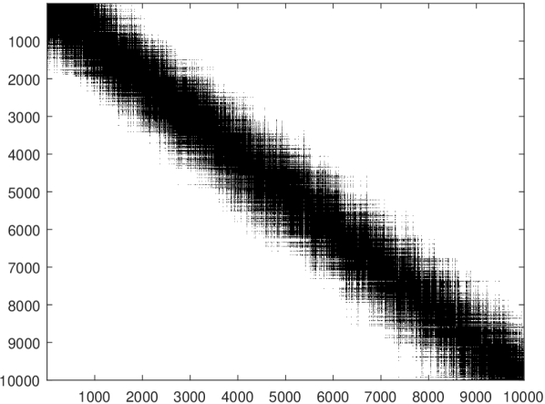
Stage 1

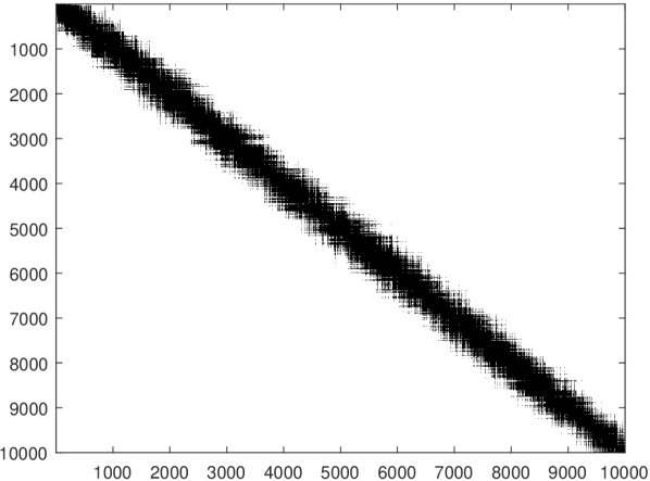
Stage 2

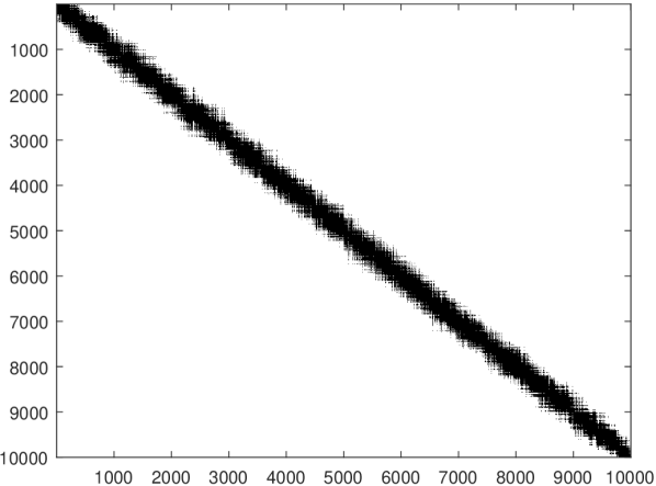
Stage 3

Figure 2: The uncertainty regions $\mathcal{R}^{(t)}$ at stages $t=1,2,3$ of the MS algorithm. The two axes represent the indices of the items. A black pixel at $(i,j)$ indicates that $(i,j)\in\mathcal{R}^{(t)}$, i.e., the algorithm is not certain about the relative order of item $i$ and item $j$ at stage $t$. A white pixel indicates the opposite.

To gain further intuition about the MS algorithm, we consider the set $I^{(t)}(i)$ defined in the algorithm. At stage $t$ of the algorithm, the set $I^{(t)}(i)$ consists of all indices $j$ for which we are not certain about the relative order of item $i$ and item $j$. The proof of Theorem 2 essentially shows that the uncertainty set $I^{(t)}(i)$ is shrinking as the algorithm proceeds. To verify this intuition, in Figure 2 we plot the uncertainty regions

$$\mathcal{R}^{(t)}:\,=\big{\{}(i,j)\in[n]^{2}:i\in[n],\,j\in I^{(t)}(i)\big{\}}$$

at stages $t=1,2,3$ of the MS algorithm, for $n=10,000$ and $N=\binom{n}{2}$. The items are ordered according to $\pi^{*}=\mathsf{id}$ for visibility of the region. As exhibited in the plots, the uncertainty region is indeed shrinking as the algorithm proceeds.

5 The symmetric group and inversions

Before proving the main results for the noisy sorting model, we study the metric entropy of the symmetric group $\mathfrak{S}_{n}$ with respect to the Kendall tau distance. Counting permutations subject to constraints in terms of the Kendall tau distance is of theoretical importance and has interesting applications, e.g., in coding theory (see, e.g, Barg and Mazumdar, 2010; Mazumdar et al., 2013). We present the results in terms of metric entropy, which easily applies to the noisy sorting problem and may find further applications in statistical problems involving permutations.

For $\varepsilon>0$ and $S\subseteq\mathfrak{S}_{n}$, let $N(S,\varepsilon)$ and $D(S,\varepsilon)$ denote respectively the $\varepsilon$-covering number and the $\varepsilon$-packing number of $S$ with respect to the Kendall tau distance. The following main result of this section provides bounds on the metric entropy of balls in $\mathfrak{S}_{n}$.

Proposition 3

Consider the ball $\mathcal{B}(\pi,r)=\{\sigma\in\mathfrak{S}_{n}:d_{\mathsf{KT}}(\pi,\sigma)\leq r\}$ centered at $\pi\in\mathfrak{S}_{n}$ with radius $r\in(0,\binom{n}{2}]$. We have that for $\varepsilon\in(0,r)$,

$$n\log\big{(}\frac{r}{n+\varepsilon}\big{)}-2n \leq\log N(\mathcal{B}(\pi,r),\varepsilon)\leq\log D(\mathcal{B}(\pi,r),\varepsilon)\leq n\log\big{(}\frac{2n+2r}{\varepsilon}\big{)}+2n\,.$$

We now discuss some high-level implications of Proposition 3. Note that if $n\lesssim\varepsilon<r\leq\binom{n}{2}$, the lemma states that the $\varepsilon$-metric entropy of a ball of radius $r$ in the Kendall tau distance scales as $n\log\frac{r}{\varepsilon}$. In other words, the symmetric group $\mathfrak{S}_{n}$ equipped with the Kendall tau metric is a doubling space with doubling dimension $\Theta(n)$. One of the main messages of the current work is that although $\log|\mathfrak{S}_{n}|=\log(n!)\asymp n\log n$, the intrinsic dimension of $\mathfrak{S}_{n}$ is $\Theta(n)$, which explains the absence of logarithmic factor in the minimax rate.

To start the proof, we first recall a useful tool for counting permutations, the inversion table. Formally, the inversion table $b_{1},\dots,b_{n}$ of a permutation $\pi\in\mathfrak{S}_{n}$ is defined by

$$b_{i}=\sum_{j:i<j}\mathbbm{1}\big{(}\pi(i)>\pi(j)\big{)}$$

for $i\in[n]$. Clearly, we have that $b_{i}\in\{0,1,\dots,n-i\}$ and $d_{\mathsf{KT}}(\pi,\mathsf{id})=\sum_{i=1}^{n}b_{i}$. It is easy to reconstruct a unique permutation using an inversion table with $b_{i}\in\{0,1,\dots,n-i\},i\in[n]$, so the set of inversion tables is bijective to $\mathfrak{S}_{n}$ via this relation; see, e.g., Mahmoud (2000). We use this bijection to bound the number of permutations that differ from the identity by at most $k$ inversions. The following lemma appears in a different form in Barg and Mazumdar (2010). We provide a simple proof here for completeness.

Lemma 4

For $0\leq k\leq\binom{n}{2}$, we have that

$$n\log(k/n)-n\leq\log\big{|}\{\pi\in\mathfrak{S}_{n}:d_{\mathsf{KT}}(\pi,\mathsf{id})\leq k\}\big{|}\leq n\log(1+k/n)+n\,.$$

Proof  According to the discussion above, the cardinality $\big{|}\{\pi\in\mathfrak{S}_{n}:d_{\mathsf{KT}}(\pi,\mathsf{id})\leq k\}\big{|}$, which we denote by $L$, is equal to the number of inversion tables $b_{1},\dots,b_{n}$ where $b_{i}\in\{0,1,\dots,n-i\}$ such that $\sum_{i=1}^{n}b_{i}\leq k$. On the one hand, if $b_{i}\leq\lfloor k/n\rfloor$ for all $i\in[n]$, then $\sum_{i=1}^{n}b_{i}\leq k$, so a lower bound on $L$ is given by

$$L \geq\prod_{i=1}^{n}(\lfloor k/n\rfloor+1)\land(n-i+1)$$

$$\geq\prod_{i=1}^{n-\lfloor k/n\rfloor}(\lfloor k/n\rfloor+1)\prod_{i=n-\lfloor k/n\rfloor+1}^{n}(n-i+1)$$

$$\geq(k/n)^{n-k/n}\lfloor k/n\rfloor!\,.$$

Using Stirling’s approximation, we see that

$$\log L \geq n\log(k/n)-(k/n)\log(k/n)+\lfloor k/n\rfloor\log\lfloor k/n\rfloor-\lfloor k/n\rfloor$$

$$\geq n\log(k/n)-n\,.$$

On the other hand, if $b_{i}$ is only required to be a nonnegative integer for each $i\in[n]$, then we can use a standard “stars and bars” counting argument (Feller, 1968) to get an upper bound of the form

$$L\leq\binom{n+k}{n}\leq e^{n}(1+k/n)^{n}\,.$$

Taking the logarithm finishes the proof.  

We are ready to prove Proposition 3.

Proof [of Proposition 3] The relation between the covering and the packing number is standard.

We employ a standard volume argument to control these numbers. Let $\mathcal{P}$ be a $2\varepsilon$-packing of $\mathcal{B}(\pi,r)$ so that the balls $\mathcal{B}(\sigma,\varepsilon)$ are disjoint for $\sigma\in\mathcal{P}$. Moreover, by the triangle inequality, $\mathcal{B}(\sigma,\varepsilon)\subseteq\mathcal{B}(\pi,r+\varepsilon)$ for each $\sigma\in\mathcal{P}$. By the invariance of the Kendall tau distance under composition, Lemma 4 yields

$$\log D(\mathcal{B}(\pi,r),2\varepsilon) \leq n\log(1+r/n)+n-n\log(\varepsilon/n)+n$$

$$=n\log\big{(}\frac{n+r}{\varepsilon}\big{)}+2n\,.$$

On the other hand, if $\mathcal{N}$ is an $\varepsilon$-net of $\mathcal{B}(\pi,r)$, then the set of balls $\{\mathcal{B}(\sigma,\varepsilon)\}_{\sigma\in\mathcal{N}}$ covers $\mathcal{B}(\pi,r)$. By Lemma 4, we obtain

$$\log N(\mathcal{B}(\pi,r),\varepsilon) \geq\log|\mathcal{B}(\pi,r)|-\log|\mathcal{B}(\sigma,\varepsilon)|$$

$$\geq n\log(r/n)-n-n\log(1+\varepsilon/n)-n$$

$$=n\log\big{(}\frac{r}{n+\varepsilon}\big{)}-2n\,,$$

as claimed.  

The lower bound on the packing number in Proposition 3 becomes vacuous when $r$ and $\varepsilon$ are smaller than $n$, so we complement it with the following result, which is useful for proving minimax lower bounds.

Lemma 5

Consider the ball $\mathcal{B}(\pi,r)$ where $r<n/2$. We have that

$$\log N(\mathcal{B}(\pi,r),r/4)\geq\frac{r}{5}\log\frac{n}{r}\,.$$

Proof  Without loss of generality, we may assume that $\pi=\mathsf{id}$ and $n$ is even. The sparse Varshamov-Gilbert bound (Massart, 2007, Lemma 4.10) states that there exists a set $\mathcal{S}$ of $r$-sparse vectors in $\{0,1\}^{n/2}$, such that $\log|\mathcal{S}|\geq\frac{r}{5}\log\frac{n}{r}$ and any two distinct vectors in $\mathcal{S}$ are separated by at least $r/2$ in the Hamming distance. We now map every $v\in\mathcal{S}$ to a permutation $\pi\in\mathcal{B}(\mathsf{id},r)$ by defining

1. $\pi(2i-1)=2i-1$ and $\pi(2i)=2i$ if $v(i)=0$, and

2. $\pi(2i-1)=2i$ and $\pi(2i)=2i-1$ if $v(i)=1$,

for $i\in[n]$. Note that $\pi\in\mathcal{B}(\mathsf{id},r)$ because $\pi$ swaps at most $r$ adjacent pairs. Denote by $\mathcal{P}$ the image of $\mathcal{S}$ under this mapping. Since the Hamming distance between any two distinct vectors in $\mathcal{S}$ is lower bounded by $r/2$, we see that $d_{\mathsf{KT}}(\pi,\sigma)\geq r/2$ for any distinct $\pi,\sigma\in\mathcal{P}$. Thus $\mathcal{P}$ is an $r/2$-packing of $\mathcal{B}(\mathsf{id},r)$. By construction, $|\mathcal{P}|=|\mathcal{S}|\geq\frac{r}{5}\log\frac{n}{r}$, so we can use the standard relation $D(\mathcal{B}(\mathsf{id},r),r/2)\leq N(\mathcal{B}(\mathsf{id},r),r/4)$ to complete the proof.  

6 Proofs of the main results

This section is devoted to the proofs of our main results. We start with a lemma giving useful tail bounds for the binomial distribution.

Lemma 6

Suppose that $X$ has the Binomial distribution $\mathsf{Bin}(N,p)$ where $N\in\mathbbm{Z}_{+}$ and $p\in(0,1)$. Then for $r\in(0,p)$ and $s\in(p,1)$, we have

1. $\mathbbm{P}(X\leq rN)\leq\exp\big{(}-N\frac{(p-r)^{2}}{2p(1-r)}\big{)},$ and

2. $\mathbbm{P}(X\geq sN)\leq\exp\big{(}-N\frac{(p-s)^{2}}{2s(1-p)}\big{)}.$

Proof  First, for $0<q<p<1$, by the definition of the Kullback-Leibler divergence, we have

$$\mathsf{KL}\big{(}\mathsf{Ber}(p)\|\mathsf{Ber}(q)\big{)} =p\log\frac{p}{q}+(1-p)\log\frac{1-p}{1-q}=\int_{q}^{p}\big{(}\frac{p}{x}-\frac{1-p}{1-x}\big{)}\,dx$$

$$=\int_{q}^{p}\frac{p-x}{x(1-x)}\,dx\geq\int_{q}^{p}\frac{p-x}{p(1-q)}\,dx=\frac{(p-q)^{2}}{2p(1-q)}\,.$$ (6.1)

Thus we also have

$$\mathsf{KL}\big{(}\mathsf{Ber}(q)\|\mathsf{Ber}(p)\big{)}=\mathsf{KL}\big{(}\mathsf{Ber}(1-q)\|\mathsf{Ber}(1-p)\big{)}\geq\frac{(p-q)^{2}}{2p(1-q)}\,.$$ (6.2)

Moreover, by Theorem 1 of Arratia and Gordon (1989) and symmetry, it holds that

1. $\mathbbm{P}(X\leq rN)\leq\exp(-N\mathsf{KL}(\mathsf{Ber}(r)\|\mathsf{Ber}(p))),$ and

2. $\mathbbm{P}(X\geq sN)\leq\exp(-N\mathsf{KL}(\mathsf{Ber}(s)\|\mathsf{Ber}(p))).$

The claimed tail bounds hence follow from (6.1) and (6.2).  

6.1 Proof of Theorem 1

First, to achieve optimal upper bounds, we consider a variant of maximum likelihood estimation. Fix $\lambda\in(0,1/2),p\in(0,1]$ and define $\varphi=np^{-1}\lambda^{-2}$ in the case of sampling model ($O_{1}$), and $\varphi=n^{3}N^{-1}\lambda^{-2}$ in the case of sampling model ($O_{2}$). If $\lambda$ or $p$ is unknown, one may learn these scalar parameters easily from the observations and define $\varphi$ using the estimated values. For readability, we assume that they are given to avoid these technical complications.

Let $\mathcal{P}$ be a maximal $\varphi$-packing (and thus a $\varphi$-net) of the symmetric group $\mathfrak{S}_{n}$ with respect to $d_{\mathsf{KT}}$. Consider the following estimator:

$$\hat{\pi}\in\operatorname*{argmax}_{\pi\in\mathcal{P}}\sum_{\pi(i)>\pi(j)}A_{i,j}\,.$$ (6.3)

It is easy to see that $\hat{\pi}$ is the MLE of $\pi^{*}$ over $\mathcal{P}$. Such an estimator is often called sieve estimator (see, e.g. Le Cam, 1986) in the statistics literature. The estimator $\hat{\pi}$ satisfies the following upper bounds.

Theorem 7

Consider the noisy sorting model with underlying permutation $\pi^{*}$ and probability matrix $M\in\mathcal{M}_{n}(\lambda)$ where $\lambda\in(0,\frac{1}{2})$. Then, with probability at least $1-e^{-n/8}$, the estimator $\hat{\pi}$ defined in (6.3) satisfies

$$d_{\mathsf{KT}}(\hat{\pi},\pi^{*})\lesssim\left\{\begin{array}[]{ll}\displaystyle\frac{n}{p\lambda^{2}}\land n^{2}&\text{in model \ref{model:1}}\\ \displaystyle\frac{n^{3}}{N\lambda^{2}}\land n^{2}&\text{in model \ref{model:2}}\,.\end{array}\right.$$

By integrating the tail probabilities of the above bounds, we easily obtain bounds on the expectation $\mathbbm{E}[d_{\mathsf{KT}}(\hat{\pi},\pi^{*})]$ of the same order, which then prove the upper bounds in Theorem 1. One may wonder whether the rate in Theorem 7 can be achieved by the MLE $\check{\pi}$ over $\mathfrak{S}_{n}$ defined by

$$\check{\pi}\in\operatorname*{argmax}_{\pi\in\mathfrak{S}_{n}}\sum_{\pi(i)>\pi(j)}A_{i,j}\,.$$

Our current techniques only allow us to prove bounds on $d_{\mathsf{KT}}(\check{\pi},\pi^{*})$ that incur an extra factor $\log(1/p\lambda)$ (resp. $\log(n^{2}/N\lambda)$) in model ($O_{1}$) (resp. ($O_{2}$)). It is unclear whether these logarithmic factors can be removed for the MLE.

Proof [of Theorem 7] We assume that $n$ is lower bounded by a constant without loss of generality, and note that the bounds of order $n^{2}$ are trivial. The proof is split into four parts to improve readability.

Basic setup.

Since $\mathcal{P}$ is a maximal $\varphi$-packing of $\mathfrak{S}_{n}$, it is also a $\varphi$-net and thus there exists $\tilde{\pi}\in\mathcal{P}$ such that $\mathfrak{D}:\,=d_{\mathsf{KT}}(\tilde{\pi},\pi^{*})\leq\varphi$. By definition of $\hat{\pi}$, $\sum_{\hat{\pi}(i)<\hat{\pi}(j)}A_{i,j}\leq\sum_{\tilde{\pi}(i)<\tilde{\pi}(j)}A_{i,j}.$ Canceling concordant pairs $(i,j)$ under $\hat{\pi}$ and $\tilde{\pi}$, we see that

$$\sum_{\hat{\pi}(i)<\hat{\pi}(j),\,\tilde{\pi}(i)>\tilde{\pi}(j)}A_{i,j}\leq\sum_{\hat{\pi}(i)>\hat{\pi}(j),\,\tilde{\pi}(i)<\tilde{\pi}(j)}A_{i,j}\,.$$

Splitting the summands according to $\pi^{*}$ yields that

$$\sum_{\begin{subarray}{c}\scriptscriptstyle\hat{\pi}(i)<\hat{\pi}(j),\\ \scriptscriptstyle\tilde{\pi}(i)>\tilde{\pi}(j),\\ \scriptscriptstyle\pi^{*}(i)<\pi^{*}(j)\end{subarray}}A_{i,j}+\sum_{\begin{subarray}{c}\scriptscriptstyle\hat{\pi}(i)<\hat{\pi}(j),\\ \scriptscriptstyle\tilde{\pi}(i)>\tilde{\pi}(j),\\ \scriptscriptstyle\pi^{*}(i)>\pi^{*}(j)\end{subarray}}A_{i,j}\leq\sum_{\begin{subarray}{c}\scriptscriptstyle\hat{\pi}(i)>\hat{\pi}(j),\\ \scriptscriptstyle\tilde{\pi}(i)<\tilde{\pi}(j),\\ \scriptscriptstyle\pi^{*}(i)<\pi^{*}(j)\end{subarray}}A_{i,j}+\sum_{\begin{subarray}{c}\scriptscriptstyle\hat{\pi}(i)>\hat{\pi}(j),\\ \scriptscriptstyle\tilde{\pi}(i)<\tilde{\pi}(j),\\ \scriptscriptstyle\pi^{*}(i)>\pi^{*}(j)\end{subarray}}A_{i,j}\,.$$

Since $A_{i,j}\geq 0$, we may drop the leftmost term and drop the condition $\hat{\pi}(i)>\hat{\pi}(j)$ in the rightmost term to obtain that

$$\sum_{\begin{subarray}{c}\scriptscriptstyle\hat{\pi}(i)<\hat{\pi}(j),\\ \scriptscriptstyle\tilde{\pi}(i)>\tilde{\pi}(j),\\ \scriptscriptstyle\pi^{*}(i)>\pi^{*}(j)\end{subarray}}A_{i,j}\leq\sum_{\begin{subarray}{c}\scriptscriptstyle\hat{\pi}(i)>\hat{\pi}(j),\\ \scriptscriptstyle\tilde{\pi}(i)<\tilde{\pi}(j),\\ \scriptscriptstyle\pi^{*}(i)<\pi^{*}(j)\end{subarray}}A_{i,j}+\sum_{\begin{subarray}{c}\tilde{\pi}(i)<\tilde{\pi}(j),\\ \pi^{*}(i)>\pi^{*}(j)\end{subarray}}A_{i,j}\,.$$ (6.4)

This inequality is crucial to proving that $\hat{\pi}$ is close to $\pi^{*}$ with high probability.

To set up the rest of the proof, we define, for $\pi\in\mathcal{P}$,

$$L_{\pi} =|\{(i,j)\in[n]^{2}:\pi(i)<\pi(j),\tilde{\pi}(i)>\tilde{\pi}(j),\pi^{*}(i)>\pi^{*}(j)\}|$$

$$=|\{(i,j)\in[n]^{2}:\pi(i)>\pi(j),\tilde{\pi}(i)<\tilde{\pi}(j),\pi^{*}(i)<\pi^{*}(j)\}|\,.$$

Moreover, define the random variables

$$X_{\pi}=\sum_{\begin{subarray}{c}\scriptscriptstyle\pi(i)<\pi(j),\\ \scriptscriptstyle\tilde{\pi}(i)>\tilde{\pi}(j),\\ \scriptscriptstyle\pi^{*}(i)>\pi^{*}(j)\end{subarray}}A_{i,j}\,,\quad Y_{\pi}=\sum_{\begin{subarray}{c}\scriptscriptstyle\pi(i)>\pi(j),\\ \scriptscriptstyle\tilde{\pi}(i)<\tilde{\pi}(j),\\ \scriptscriptstyle\pi^{*}(i)<\pi^{*}(j)\end{subarray}}A_{i,j}\,,\quad\text{and}\quad Z=\sum_{\begin{subarray}{c}\scriptscriptstyle\tilde{\pi}(i)<\tilde{\pi}(j),\\ \scriptscriptstyle\pi^{*}(i)>\pi^{*}(j)\end{subarray}}A_{i,j}.$$

We will prove that the random process $X_{\pi}-Y_{\pi}-Z$ is positive with high probability if $\pi$ is too far from $\tilde{\pi}$. However, (6.4) says precisely that $X_{\hat{\pi}}-Y_{\hat{\pi}}-Z\leq 0$, so that $\pi$ must be close to $\tilde{\pi}$ which is in turn close to $\pi^{*}$.

The case $M=M^{*}_{n}(\lambda)$ under sampling model ($O_{1}$).

Consider model ($O_{1}$) of sampling without replacement, and suppose that $M=M^{*}_{n}(\lambda)$ first. For a pair $(i,j)$ with $\pi^{*}(i)>\pi^{*}(j)$, the entry $A_{i,j}$ has distribution $\mathsf{Ber}\big{(}p(\frac{1}{2}+\lambda)\big{)}$, since item $i$ and item $j$ are compared with probability $p$ and conditioned on them being compared, item $i$ wins with probability $\frac{1}{2}+\lambda$. Moreover, $A_{i,j}$ is independent from any other $A_{k,\ell}$ with $\pi^{*}(k)>\pi^{*}(\ell)$. Hence $X_{\pi}$ has distribution $\mathsf{Bin}\big{(}L_{\pi},p(\frac{1}{2}+\lambda)\big{)}$. Similarly, $Y_{\pi}$ has distribution $\mathsf{Bin}\big{(}L_{\pi},p(\frac{1}{2}-\lambda)\big{)}$, and $Z$ has distribution $\mathsf{Bin}\big{(}\mathfrak{D},p(\frac{1}{2}+\lambda)\big{)}$. Therefore, Lemma 6 implies that

1. $\mathbbm{P}\big{(}X_{\pi}\leq L_{\pi}p(\frac{1}{2}+\frac{1}{2}\lambda)\big{)}\leq\exp\big{(}-L_{\pi}p\lambda^{2}/8\big{)}$, and

2. $\mathbbm{P}\big{(}Y_{\pi}\geq L_{\pi}p(\frac{1}{2}-\frac{1}{2}\lambda)\big{)}\leq\exp\big{(}-L_{\pi}p\lambda^{2}/8\big{)}.$

Then we have that

$$\mathbbm{P}(X_{\pi}-Y_{\pi}\leq L_{\pi}p\lambda)\leq 2\exp\big{(}-L_{\pi}p\lambda^{2}/8\big{)}\,.$$ (6.5)

For an integer $r\in[C\varphi,\binom{n}{2}]$ where $C$ is a sufficiently large constant to be chosen, consider the slice $\mathcal{S}_{r}=\{\pi\in\mathcal{P}:L_{\pi}=r\}$. Note that if $\pi\in\mathcal{S}_{r}$, then

$$d_{\mathsf{KT}}(\pi,\pi^{*}) =|\{(i,j):\hat{\pi}(i)<\hat{\pi}(j),\pi^{*}(i)>\pi^{*}(j)\}|$$

$$\leq|\{(i,j):\hat{\pi}(i)<\hat{\pi}(j),\tilde{\pi}(i)>\tilde{\pi}(j),\pi^{*}(i)>\pi^{*}(j)\}|$$

$$\quad\ +|\{(i,j):\tilde{\pi}(i)<\tilde{\pi}(j),\pi^{*}(i)>\pi^{*}(j)\}|$$

$$=L_{\pi}+d_{\mathsf{KT}}(\tilde{\pi},\pi^{*})\leq r+\varphi\,.$$ (6.6)

Since $\mathcal{P}$ is a $\varphi$-packing of $\mathfrak{S}_{n}$ and $\mathcal{S}_{r}\subseteq\mathcal{P}$, we see that $|\mathcal{S}_{r}|$ is bounded by the $\varphi$-packing number of the ball $\mathcal{B}(\pi^{*},r+\varphi)$ in the Kendall tau distance. Therefore, Proposition 3 gves

$$\log|\mathcal{S}_{r}|\leq n\log\frac{2n+2r+2\varphi}{\varphi}+2n\leq n\log\frac{45r}{\varphi}\,.$$

By (6.5) and a union bound over $\mathcal{S}_{r}$, we see that $\min_{\pi\in\mathcal{S}_{r}}(X_{\pi}-Y_{\pi})>cL_{\pi}p$ with probability at least

$$\quad\ 1-\exp\Big{(}n\log\frac{45r}{\varphi}+\log 2-\frac{rp\lambda^{2}}{8}\Big{)}$$

$$=1-\exp\Big{(}n\log\frac{45r}{\varphi}+\log 2-\frac{rn}{8\varphi}\Big{)}\geq 1-\exp(-2n)\,,$$

where the inequality holds because $r/\varphi\geq C$ for a sufficiently large constant $C$. Then a union bound over integers $r\in[C\varphi,\binom{n}{2}]$ yields that $X_{\pi}-Y_{\pi}>cL_{\pi}p$ for all $\pi\in\mathcal{P}$ such that $L_{\pi}\geq C\varphi$ with probability at least $1-e^{-n}$.

Furthermore, since $Z\sim\mathsf{Bin}\big{(}\mathfrak{D},p(\frac{1}{2}+\lambda)\big{)}$ and $\mathfrak{D}\leq\varphi$, Lemma 6 gives that

$$\mathbbm{P}(Z\geq 2\varphi p)\leq\exp(-\varphi p/4)\leq\exp(-n/4)\,.$$

Combining the bounds on $X_{\pi}-Y_{\pi}$ and $Z$, we conclude that with probability at least $1-e^{-n/8}$,

$$X_{\pi}-Y_{\pi}-Z>cC\varphi p-2\varphi p>0$$

for all $\pi\in\mathcal{P}$ with $L_{\pi}\geq C\varphi$, as long as $C>2/c$.

We have seen in (6.4) that $X_{\hat{\pi}}-Y_{\hat{\pi}}-Z\leq 0$, so $L_{\hat{\pi}}\leq C\varphi$ on the above event. By (6.6), $d_{\mathsf{KT}}(\hat{\pi},\pi^{*})\leq L_{\hat{\pi}}+\varphi$ on the same event, which completes the proof for the model ($O_{1}$).

The general case under sampling model ($O_{1}$).

Let us continue to use $X_{\pi}$, $Y_{\pi}$ and $Z$ to denote the above random variables under the noisy sorting model $\mathcal{P}$ with probability matrix $M^{*}_{n}(\lambda)$, and use $\tilde{X}_{\pi}$, $\tilde{Y}_{\pi}$ and $\tilde{Z}$ to denote the corresponding random variables under a general noisy sorting model $\tilde{\mathcal{P}}$ with $M\in\mathcal{M}_{n}(\lambda)$. We couple the two models such that:

1. The sets of pairs of items being compared are the same (and if a pair is compared multiple times, the multiplicity is also the same);

2. For each pair $(i,j)$ with $\pi^{*}(i)>\pi^{*}(j)$, if item $i$ beats item $j$ in a comparison in the model $\mathcal{P}$, then it also beats item $j$ in the corresponding comparison in the model $\tilde{\mathcal{P}}$.

The second statement can be satisfied because the results of comparisons are Bernoulli random variables and $M_{\pi^{*}(i),\pi^{*}(j)}\geq[M^{*}_{n}(\lambda)]_{\pi^{*}(i),\pi^{*}(j)}$ for all $\pi^{*}(i)>\pi^{*}(j)$, by definition. Under this coupling, we always have that $\tilde{X}_{\pi}\geq X_{\pi}$ and $\tilde{Y}_{\pi}\leq Y_{\pi}$, so the above high probability lower bound on $X_{\pi}-Y_{\pi}$ also holds on $\tilde{X}_{\pi}-\tilde{Y}_{\pi}$.

Moreover, recall the definition $\tilde{Z}=\sum_{\begin{subarray}{c}\scriptscriptstyle\tilde{\pi}(i)<\tilde{\pi}(j),\\ \scriptscriptstyle\pi^{*}(i)>\pi^{*}(j)\end{subarray}}A_{i,j},$ where $A_{i,j}\sim\mathsf{Ber}\big{(}p[M^{*}_{n}(\lambda)]_{\pi^{*}(i),\pi^{*}(j)}\big{)}$. Since $[M^{*}_{n}(\lambda)]_{\pi^{*}(i),\pi^{*}(j)}\in(0,1)$, we can couple a sequence of i.i.d. $B_{i,j}\sim\mathsf{Ber}(p)$ with the $A_{i,j}$’s in such a way that $B_{i,j}=1$ whenever $A_{i,j}=1$. Define $W=\sum_{\begin{subarray}{c}\scriptscriptstyle\tilde{\pi}(i)<\tilde{\pi}(j),\\ \scriptscriptstyle\pi^{*}(i)>\pi^{*}(j)\end{subarray}}B_{i,j}$. Then we see that $W\sim\mathsf{Bin}(\mathfrak{D},p)$ and $W\geq\tilde{Z}$. Since $\mathfrak{D}\leq\varphi$, Lemma 6 gives

$$\mathbbm{P}(W\geq 2\varphi p)\leq\exp(-\varphi p/4)\leq\exp(-n/4)\,.$$

Thus $\tilde{Z}$ is subject to the same high probability upper bound as $Z$. Therefore, the proof for the model $\mathcal{P}$ also works to show the desired bound for the model $\tilde{\mathcal{P}}$.

Sampling model ($O_{2}$).

The proof for model ($O_{2}$) of sampling with replacement is essentially the same, except the part of probability bounds where we assume $M=M^{*}_{n}(\lambda)$. We now demonstrate the differences in detail. For a single pairwise comparison sampled uniformly from the possible $\binom{n}{2}$ pairs, the probability that

1. the chosen pair $(i,j)$ satisfies $\pi(i)<\pi(j)$, $\tilde{\pi}(i)>\tilde{\pi}(j)$ and $\pi^{*}(i)>\pi^{*}(j)$, and

2. item $i$ wins the comparison,

is equal to $L_{\pi}\binom{n}{2}^{-1}(\frac{1}{2}+\lambda)$. By definition, $X_{\pi}$ is the number of times the above event happens if $N$ independent pairwise comparisons take place, so $X_{\pi}\sim\mathsf{Bin}\big{(}N,L_{\pi}\binom{n}{2}^{-1}(\frac{1}{2}+\lambda)\big{)}$. Similarly, we have $Y_{\pi}\sim\mathsf{Bin}\big{(}N,L_{\pi}\binom{n}{2}^{-1}(\frac{1}{2}-\lambda)\big{)}$ and $Z\sim\mathsf{Bin}\big{(}N,\mathfrak{D}\binom{n}{2}^{-1}(\frac{1}{2}+\lambda)\big{)}$. Hence Lemma 6 gives that

1. $\mathbbm{P}\big{(}X_{\pi}\leq L_{\pi}N\binom{n}{2}^{-1}(\frac{1}{2}+\frac{1}{2}\lambda)\big{)}\leq\exp\big{(}-L_{\pi}N\binom{n}{2}^{-1}\lambda^{2}/8\big{)},$

2. $\mathbbm{P}\big{(}Y_{\pi}\geq L_{\pi}N\binom{n}{2}^{-1}(\frac{1}{2}-\frac{1}{2}\lambda)\big{)}\leq\exp\big{(}-L_{\pi}N\binom{n}{2}^{-1}\lambda^{2}/8\big{)},$ and

3. $\mathbbm{P}\big{(}Z\geq 2\varphi N\binom{n}{2}^{-1}\big{)}\leq\exp\big{(}-\varphi N\binom{n}{2}^{-1}/4\big{)}\,.$

Note that if we set $p=N\binom{n}{2}^{-1}$, then the tail bounds above are exactly the same as those for the model ($O_{1}$). Therefore, replacing $p$ by $N\binom{n}{2}^{-1}$ everywhere in the above proof, we then obtain the desired bound for the model ($O_{2}$).  

Next, we turn to the lower bounds. Let $\mathbbm{P}_{\pi^{*}}=\mathbbm{P}_{\pi^{*},M^{*}_{n}(\lambda)}$ denote the probability distribution of the observations in the noisy sorting model with underlying permutation $\pi^{*}\in\mathfrak{S}_{n}$ and probability matrix $M^{*}_{n}(\lambda)$, where $\lambda\in(0,\frac{1}{2})$. We prove the following stronger statement which clearly implies the lower bounds in Theorem 1.

Theorem 8

For the sampling model ($O_{1}$), suppose we have $\lambda\in(0,\frac{1}{2})$ and $p\in(0,1]$ such that $p\log\frac{1}{1-2\lambda}\leq C$ for some constant $C>0$. Then it holds that

$$\min_{\tilde{\pi}}\max_{\pi^{*}\in\mathfrak{S}_{n}}\,\mathbbm{P}_{\pi^{*}}\Big{(}d_{\mathsf{KT}}(\tilde{\pi},\pi^{*})\gtrsim\frac{n}{p\lambda^{2}}\land\frac{n}{p\log\frac{1}{1-2\lambda}}\land n^{2}\Big{)}\geq c\,,$$

where the minimum is taken minimized over all permutation estimators $\tilde{\pi}\in\mathfrak{S}_{n}$ that are measurable with respect to the observations and $c$ is a universal positive constant. Similarly, for the sampling model ($O_{2}$), if we have $Nn^{-2}\log\frac{1}{1-2\lambda}\leq C$, then it holds that

$$\min_{\tilde{\pi}}\max_{\pi^{*}\in\mathfrak{S}_{n}}\,\mathbbm{P}_{\pi^{*}}\Big{(}d_{\mathsf{KT}}(\tilde{\pi},\pi^{*})\gtrsim\frac{n^{3}}{N\lambda^{2}}\land\frac{n^{3}}{N\log\tfrac{1}{1-2\lambda}}\land n^{2}\Big{)}\geq c\,.$$

Compared to the lower bounds in Theorem 1, the above lower bounds hold in probability, weaken the condition that $\lambda$ is bounded away from $1/2$ and only require maximizing $\pi^{*}$ instead of both $\pi^{*}$ and $M$, and are therefore stronger.

One key ingredient in proving lower bounds is to relate the Kullback-Leibler divergence between model distributions to the distance measuring the error (see, e.g., Tsybakov, 2009, Chapter 2). This is achieved in the following lemma for both sampling models.

Lemma 9

Fix $\pi,\sigma\in\mathfrak{S}_{n}$ and $\lambda\in(0,\frac{1}{2})$. We denote by $\mathbbm{P}_{\pi}$ the probability distribution of the noisy sorting model with underlying permutation $\pi$. Then for the sampling model ($O_{1}$) we have

$$\mathsf{KL}(\mathbbm{P}_{\pi}\|\mathbbm{P}_{\sigma})=2\,d_{\mathsf{KT}}(\pi,\sigma)\,p\lambda\log\frac{1+2\lambda}{1-2\lambda}\,,$$

and for the sampling model ($O_{2}$) we have

$$\mathsf{KL}(\mathbbm{P}_{\pi}\|\mathbbm{P}_{\sigma})=2\,d_{\mathsf{KT}}(\pi,\sigma)\,N\binom{n}{2}^{-1}\lambda\log\frac{1+2\lambda}{1-2\lambda}\,.$$

Proof  First, we consider model ($O_{1}$) of sampling without replacement. For $i\neq j$, let $\mathbbm{P}_{\pi}^{(i,j)}$ denote the distribution of outcomes between $i$ and $j$, or more formally, the distribution of $N_{i,j}$ and $A_{i,j}$. For a pair $(i,j)$ such that $\pi(i)>\pi(j)$ and $\sigma(i)>\sigma(j)$, the distributions $\mathbbm{P}_{\pi}^{(i,j)}$ and $\mathbbm{P}_{\sigma}^{(i,j)}$ are indistinguishable. For $(i,j)$ such that $\pi(i)>\pi(j)$ and $\sigma(i)<\sigma(j)$, the probability that $i$ and $j$ are not compared stays the same, but the probability that they are compared and $i$ wins the comparison is $p(\frac{1}{2}+\lambda)$ under $\mathbbm{P}_{\pi}^{(i,j)}$ while it is $p(\frac{1}{2}-\lambda)$ under $\mathbbm{P}_{\sigma}^{(i,j)}$. A symmetric statement holds for the probability that they are compared and $j$ wins the comparison. Therefore, we obtain that

$$\mathsf{KL}(\mathbbm{P}_{\pi}^{(i,j)}\|\mathbbm{P}_{\sigma}^{(i,j)}) =p(1/2+\lambda)\log\frac{1/2+\lambda}{1/2-\lambda}+p(1/2-\lambda)\log\frac{1/2-\lambda}{1/2+\lambda}$$

$$=2p\lambda\log\frac{1+2\lambda}{1-2\lambda}\,.$$

It follows from the chain rule that

$$\mathsf{KL}(\mathbbm{P}_{\pi}\|\mathbbm{P}_{\sigma})=\sum_{\pi(i)>\pi(j),\,\sigma(i)<\sigma(j)}\mathsf{KL}(\mathbbm{P}_{\pi}^{i,j}\|\mathbbm{P}_{\sigma}^{i,j})=2\,d_{\mathsf{KT}}(\pi,\sigma)\,p\lambda\log\frac{1+2\lambda}{1-2\lambda}\,,$$

which proves the claimed bound.

Next, we move on to model ($O_{2}$) of sampling with replacement. In this case, for the noisy sorting model with underlying permutation $\pi$, we let $\mathbb{Q}_{\pi}$ denote the distribution of the outcome of a single pairwise comparison chosen uniformly from the $\binom{n}{2}$ possible pairs. Conditioned on a pair $(i,j)$ with $\pi(i)>\pi(j)$ and $\sigma(i)>\sigma(j)$ being chosen, the outcome is indistinguishable under $\mathbb{Q}_{\pi}$ and $\mathbb{Q}_{\sigma}$. On the other hand, conditioned on having chosen $(i,j)$ with $\pi(i)>\pi(j)$ and $\sigma(i)<\sigma(j)$, the probability that $i$ wins the comparison is $p(\frac{1}{2}+\lambda)$ under $\mathbb{Q}_{\pi}$ and is $p(\frac{1}{2}-\lambda)$ under $\mathbb{Q}_{\sigma}$. By the definition of the KL divergence, we have

$$\quad\ \mathsf{KL}(\mathbb{Q}_{\pi}\|\mathbb{Q}_{\sigma}) =\sum_{\pi(i)>\pi(j),\,\sigma(i)<\sigma(j)}\Big{[}\binom{n}{2}^{-1}(1/2+\lambda)\log\frac{1/2+\lambda}{1/2-\lambda}$$

$$\qquad\qquad\qquad\qquad\qquad+\binom{n}{2}^{-1}(1/2-\lambda)\log\frac{1/2-\lambda}{1/2+\lambda}\Big{]}$$

$$=2\,d_{\mathsf{KT}}(\pi,\sigma)\binom{n}{2}^{-1}\lambda\log\frac{1+2\lambda}{1-2\lambda}\,,$$

where the bound holds similarly as above. Since $N$ independent pairwise comparisons are observed and the KL divergence tensorizes, the conclusion follows.  

We are ready to prove the minimax lower bound.

Proof [of Theorem 8] Consider the sampling model ($O_{1}$). We assume that $n$ is lower bounded by a constant, and use the shorthand notation $\kappa=4p\lambda\log\frac{1+2\lambda}{1-2\lambda}$. Note that $\kappa\leq C$ for some constant $C>0$ by the assumption. Let $r=c_{0}n\kappa^{-1}\land\binom{n}{2}$ and $\varepsilon=c_{1}r$, where $c_{0}$ and $c_{1}$ are constants to be chosen. Let $\mathcal{P}$ be a maximal $\varepsilon$-packing of $\mathcal{B}(\mathsf{id},r)$, which is thus an $\varepsilon$-net by maximality. For any $\pi,\sigma\in\mathcal{P}$, we have $d_{\mathsf{KT}}(\pi,\sigma)\leq 2r$, so Lemma 9 yields

$$\mathsf{KL}(\mathbbm{P}_{\pi}\|\mathbbm{P}_{\sigma})=\frac{1}{2}\,\kappa\,d_{\mathsf{KT}}(\pi,\sigma)\leq\kappa r\leq c_{0}n\,.$$

On one hand, if $\kappa\leq c_{2}$ for a sufficiently small constant $c_{2}>0$, then $r\geq c_{0}c_{2}^{-1}n\land\binom{n}{2}$ and thus Proposition 3 implies that

$$\log|\mathcal{P}|\geq n\log\frac{r}{n+\varepsilon}-2n\geq 10\,c_{0}n\geq 10\,\mathsf{KL}(\mathbbm{P}_{\pi}\|\mathbbm{P}_{\sigma})\,,$$

where we take $c_{0}=1$ and $c_{1},c_{2}$ small enough for the inequalities to hold.

On the other hand, if $c_{2}<\kappa\leq C$, then we take $c_{1}=1/8$ and $c_{0}$ sufficiently small so that $r\leq c_{0}c_{2}^{-1}n<n/2$. Then we can apply Lemma 5 to obtain

$$\log|\mathcal{P}|\geq\frac{r}{5}\log\frac{n}{r}\geq\frac{c_{0}n}{5C}\log\frac{c_{2}}{c_{0}}\geq 10\,c_{0}n\geq 10\,\mathsf{KL}(\mathbbm{P}_{\pi}\|\mathbbm{P}_{\sigma})\,,$$

where the second inequality holds since $c_{0}C^{-1}n\leq r\leq c_{0}c_{2}^{-1}n$ and the third inequality holds for $c_{0}$ small enough.

In either case, we have $\mathsf{KL}(\mathbbm{P}_{\pi}\|\mathbbm{P}_{\sigma})\leq 0.1\log|\mathcal{P}|$. Therefore, using Tsybakov (2009, Theorem 2.5) yields the lower bound of order $r\asymp n\kappa^{-1}\land n^{2}$. Considering the limiting behavior of $\kappa$ as $\lambda\to 0$ and $\lambda\to\frac{1}{2}$ repectively, we see that $\kappa\lesssim p\lambda^{2}\lor p\log\frac{1}{1-2\lambda}$, so the claimed lower bound follows.

For the sampling model ($O_{2}$), the same argument follows if we replace $p$ with $N\binom{n}{2}^{-1}$.  

6.2 Proof of Theorem 2

Without loss of generality, assume that $\pi^{*}=\mathsf{id}$ and $n$ is even to simplify the notation. We define a score

$$s_{i}^{*}=\sum_{j\in[n]\setminus\{i\}}M_{i,j}=\lambda(2i-n-1)+(n-1)/2$$

for each $i\in[n]$, which is simply the $i$-th row sum of $M$ minus $1/2$. Analogously, we define

$$\hat{s}_{i}=\sum_{j=1}^{i-1}(\frac{1}{2}+\hat{\lambda})+\sum_{j=i+1}^{n}(\frac{1}{2}-\hat{\lambda})=\hat{\lambda}(2i-n-1)+(n-1)/2$$

for each $i\in[n]$, which is a slightly perturbed version of $s^{*}_{i}$ due to the difference between $\lambda$ and $\hat{\lambda}$. The MS algorithm is designed to refine estimates for the scores $s^{*}_{i}$ in multiple stages.

First, the estimator $\hat{\lambda}$ satisfies the following bound, which in particular implies that $\hat{s}_{i}$ is close to $s^{*}_{i}$.

Lemma 10

If $N\geq Cn\log n$, then we have $|\hat{\lambda}-\lambda|\leq C_{0}\sqrt{N^{-1}\log n}$ with probability at least $1-n^{-8}$, where $C$ and $C_{0}$ are sufficiently large universal constants.

Proof  Consider a single pairwise comparison chosen uniformly from the $\binom{n}{2}$ pairs. The probability that item $i$ is in the pair and wins the comparison is equal to $\big{(}\sum_{j\in[n]\setminus\{i\}}M_{i,j}\big{)}/\binom{n}{2}=s_{i}^{*}/\binom{n}{2}.$ Thus the random variable $S_{i}=\sum_{j=1}^{n}A_{i,j}^{\prime}$ has distribution $\mathsf{Bin}\big{(}N/2,s_{i}^{*}/\binom{n}{2}\big{)}$. Hence Lemma 6 implies that

$$\mathbbm{P}\big{(}\big{|}S_{i}-\mathbbm{E}[S_{i}]\big{|}\geq c_{1}\mathbbm{E}[S_{i}]\big{)}\leq 2\exp\big{(}-c_{2}\mathbbm{E}[S_{i}]\big{)}\leq n^{-10},$$

where the last inequality holds since $N\geq Cn\log n$, and we use $c_{1},c_{2},\dots$ to denote sufficiently small constants. A union bound shows that with probability at least $1-n^{-9}$, we have $|S_{i}-\mathbbm{E}[S_{i}]|\leq c_{1}\mathbbm{E}[S_{i}]$ for all $i\in[n]$. Denote this high probability event by $\mathcal{E}$, and we condition on $\mathcal{E}$ henceforth.

Recall that $s_{i}^{*}=2\lambda i-\lambda(n+1)+(n-1)/2$. Using that $\lambda$ is bounded away from zero, we can choose $c_{1}$ small enough so that if $i-j\geq n/4$, then $s_{i}^{*}-s_{j}^{*}>2c_{1}s_{i}^{*}$. Note that $E[S_{i}]=\frac{1}{2}Ns_{i}^{*}/\binom{n}{2}$, so $E[S_{i}]-E[S_{j}]>2c_{1}E[S_{i}]$ if $i-j\geq n/4$. Therefore, on the event $\mathcal{E}$ we have $S_{i}>S_{j}$ for all $(i,j)$ with $i-j\geq n/4$. It follows that $\tilde{\pi}(i)>\tilde{\pi}(j)$ for these pairs $(i,j)$, as $\tilde{\pi}$ is defined by sorting the scores $S_{i}$.

Next consider $(i,j)$ such that $\tilde{\pi}(i)-\tilde{\pi}(j)>n/2$. Suppose we have $i<j$. Then there exists $k\in[n]$ with $\tilde{\pi}(j)<\tilde{\pi}(k)<\tilde{\pi}(i)$ such that either $k-i\geq n/4$ or $j-k\geq n/4$, which gives a contradiction on the event $\mathcal{E}$. Therefore, it holds that $i>j$ for all pairs $(i,j)$ with $\tilde{\pi}(i)-\tilde{\pi}(j)>n/2$.

Recall that $\hat{\lambda}=\frac{2}{N}\binom{n}{2}\binom{n/2}{2}^{-1}\sum_{(i,j)\in\mathcal{I}}A_{i,j}^{\prime\prime}-\frac{1}{2},$ where $\mathcal{I}=\{(i,j)\in[n]^{2}:\tilde{\pi}(i)-\tilde{\pi}(j)>\frac{n}{2}\}$. Note that $A^{\prime\prime}$ is independent of $\mathcal{E}$, on which we have $i>j$ for all $(i,j)\in\mathcal{I}$. Similar to the argument at the beginning of the proof, the probability that a uniformly chosen pair falls in $\mathcal{I}$ and $i$ wins the comparison is $(\frac{1}{2}+\lambda)|\mathcal{I}|/\binom{n}{2}$. Hence the random variable $X:\,=\sum_{(i,j)\in\mathcal{I}}A_{i,j}^{\prime\prime}$ has distribution $\mathsf{Bin}\big{(}N/2,(\frac{1}{2}+\lambda)|\mathcal{I}|/\binom{n}{2}\big{)}$. It follows that $\mathbbm{E}[\hat{\lambda}\,|\,\mathcal{E}]=\lambda$ once we note that $|\mathcal{I}|=\binom{n/2}{2}$.

Moreover, Lemma 6 gives the bound

$$\mathbbm{P}\Big{(}\big{|}X-\mathbbm{E}[X]\big{|}\geq C_{2}\sqrt{N\log n}\,\Big{|}\,\mathcal{E}\Big{)}\leq 2\exp(-c_{3}\log n)\leq n^{-9},$$

and consequently $|\hat{\lambda}-\lambda|\leq C_{0}\sqrt{N^{-1}\log n}$ with probability at least $1-n^{-9}$ conditioned on the event $\mathcal{E}$, where $C_{2}$ and $C_{0}$ are sufficiently large constants. A union bound then completes the proof.  

We condition on the high probability event of Lemma 10 throughout the rest of the proof, so that $|\hat{\lambda}-\lambda|\leq C_{0}\sqrt{N^{-1}\log n}$ for a fixed constant $C_{0}>0$. In particular, $\hat{\lambda}$ is bounded away from zero by a universal constant since $\lambda$ is and $N\geq Cn\log n$, and $\hat{s}_{j}<\hat{s}_{i}$ iff $j<i$. We proceed with the following key lemma.

Lemma 11

Fix $t\in[T]$, $i\in[n]$ and $I\subseteq[n]$ with $i\in I$. Suppose that $|I|\geq C_{1}\frac{n^{2}T}{N}\log(nT)$ for a sufficiently large constant $C$. If we define

$$S=\frac{Tn(n-1)}{2N}\sum_{j\in I}A^{(t)}_{i,j}+\sum_{j\in[n]\setminus I,\,j<i}\big{(}\frac{1}{2}+\hat{\lambda}\big{)}+\sum_{j\in[n]\setminus I,\,j>i}\big{(}\frac{1}{2}-\hat{\lambda}\big{)}\,,$$

then it holds with probability at least $1-2(nT)^{-9}$ that

$$|S-\hat{s}_{i}|\leq(5+C_{0})n\sqrt{|I|TN^{-1}\log(nT)}\,.$$

Proof  Consider a single pairwise comparison chosen uniformly from the $\binom{n}{2}$ pairs. The probability that the chosen pair consists of item $i$ and an item in $I\setminus\{i\}$, and that item $i$ wins the comparison, is equal to $q:\,=\big{(}\sum_{j\in I\setminus\{i\}}M_{i,j}\big{)}/\binom{n}{2}.$ Thus the random variable $X:\,=\sum_{j\in I}A^{(t)}_{i,j}$ has distribution $\mathsf{Bin}(N/T,q)$. In particular, $\mathbbm{E}[X]=Nq/T=\frac{2N}{Tn(n-1)}\sum_{j\in I\setminus\{i\}}M_{i,j}$ and by Lemma 6,

$$\mathbbm{P}\Big{(}\big{|}X-\mathbbm{E}[X]\big{|}\geq\frac{rN}{T}\Big{)}\leq 2\exp\Big{(}-\frac{Nr^{2}}{2T(q+r)}\Big{)}.$$

Taking $r=6\sqrt{\frac{Tq}{N}\log(nT)}$, we see that $r\leq q$ using the assumption $|I|\geq C_{1}\frac{n^{2}T}{N}\log(nT)$, so

$$\mathbbm{P}\Big{(}\big{|}X-\mathbbm{E}[X]\big{|}\geq 6\sqrt{qNT^{-1}\log(nT)}\Big{)}\leq 2(nT)^{-9}\,.$$ (6.7)

By the definitions of $S$ and $\hat{s}_{i}$, it is straightforward to verify that

$$S-\hat{s}_{i}=\frac{Tn(n-1)}{2N}(X-\mathbbm{E}[X])+\sum_{j\in I,\,j<i}(\lambda-\hat{\lambda})+\sum_{j\in I,\,j>i}(\hat{\lambda}-\lambda)\,.$$

Therefore, we obtain from (6.7), the definition of $q$ and the fact $|I|\leq n$ that

$$|S-\hat{s}_{i}| \leq 3n(n-1)\sqrt{qTN^{-1}\log(nT)}+|I|\,|\hat{\lambda}-\lambda|$$

$$\leq 5n\sqrt{|I|TN^{-1}\log(nT)}+C_{0}|I|\sqrt{N^{-1}\log n}$$

$$\leq(5+C_{0})n\sqrt{|I|TN^{-1}\log(nT)}$$

with probability at least $1-2(nT)^{-9}$.  

To analyze the MS algorithm, we apply Lemma 11 inductively to each stage of the algorithm. Define $\mathcal{E}^{(0)}$ to be the full event. As the inductive hypothesis, we assume that on the event $\mathcal{E}^{(t-1)}$, it holds that $j<i$ for all $j\in I_{-}^{(t-1)}(i)$ and $j>i$ for all $j\in I_{+}^{(t-1)}(i)$. In particular, this holds trivially for $t=1$.

On the event $\mathcal{E}^{(t-1)}$, the score $S^{(t)}_{i}$ is exactly the quantity $S$ in Lemma 11 with $I=I^{(t-1)}(i)$. Thus the lemma shows that if $|I^{(t-1)}(i)|\geq C_{1}\frac{n^{2}T}{N}\log(nT)$ for a large enough constant $C_{1}$, then

$$|S^{(t)}_{i}-\hat{s}_{i}|\leq(5+C_{0})n\sqrt{|I^{(t-1)}(i)|TN^{-1}\log(nT)}=\tau_{i}^{(t)}/2$$ (6.8)

with probability at least $1-2(nT)^{-9}$ conditional on $\mathcal{E}^{(t-1)}$. We denote by $\mathcal{E}^{(t)}$ the sub-event of $\mathcal{E}^{(t-1)}$ that the above bound holds for all $i\in[n]$. Then $\mathbbm{P}(\mathcal{E}^{(t)}\,|\,\mathcal{E}^{(t-1)})\geq 1-(nT)^{-8}$ and we condition on $\mathcal{E}^{(t)}$ henceforth.

For any $j\in I^{(t)}_{-}(i)$, by definition $S^{(t)}_{j}-S^{(t)}_{i}<-\tau_{i}^{(t)}$, so we have $\hat{s}_{j}<\hat{s}_{i}$ and thus $j<i$. Similarly, $j>i$ for any $j\in I^{(t)}_{+}(i)$ on the event $\mathcal{E}^{(t)}$. Hence the inductive hypothesis is verified. Moreover, note that $I^{(t)}(i)=\{j\in[n]:|S^{(t)}_{j}-S^{(t)}_{i}|\leq 2\tau_{i}^{(t)}\}\subseteq\{j\in[n]:|\hat{s}_{j}-\hat{s}_{i}|\leq 3\tau_{i}^{(t)}\}.$ Since $\hat{s}_{j}-\hat{s}_{i}=2\hat{\lambda}(j-i)$ and $\hat{\lambda}$ is bounded away from zero by a universal constant, we have

$$|I^{(t)}(i)|\leq C_{2}\tau_{i}^{(t)}=C_{3}n\sqrt{|I^{(t-1)}(i)|TN^{-1}\log(nT)}\,,$$ (6.9)

where we use $C_{2},C_{3},\dots$ to denote sufficiently large constants.

Note that if we have $\alpha^{(0)}=n$ and the iterative relation $\alpha^{(t)}\leq\beta\sqrt{\alpha^{(t-1)}}$ where $\alpha^{(t)}>0$ and $\beta>0$, then it is easily seen that $\alpha^{(t)}\leq\beta^{2}n^{2^{-t}}$. We would like to obtain such a bound from the relation (6.9). Note that $\mathcal{E}^{(T)}\subseteq\mathcal{E}^{(T-1)}\subseteq\cdots\subseteq\mathcal{E}^{(0)}$ by definition and $\mathbbm{P}(\mathcal{E}^{(T)})=\prod_{t=1}^{T}\mathbbm{P}(\mathcal{E}^{(t)}\,|\,\mathcal{E}^{(t-1)})\geq 1-n^{-8}$. Conditional on $\mathcal{E}^{(T)}$, the iterative relation (6.9) thus holds for all $t\in[T]$, and we have $|I^{(0)}(i)|=n$ by definition. Since $I^{(t)}(i)$ is not updated in the algorithm once $|I^{(t)}(i)|\leq C_{1}\frac{n^{2}T}{N}\log(nT)$, we obtain that

$$|I^{(T-1)}(i)| \leq\Big{(}C_{3}^{2}\frac{n^{2}T}{N}\log(nT)n^{2^{-T+1}}\Big{)}\lor\Big{(}C_{1}\frac{n^{2}T}{N}\log(nT)\Big{)}$$

$$\leq C_{4}\frac{n^{2}}{N}(\log n)(\log\log n)\,,$$

where the last bound holds because we take $T=\lfloor\log\log n\rfloor$. Hence it follows from (6.8) that

$$|S^{(T)}_{i}-\hat{s}_{i}|\leq C_{5}n^{2}N^{-1}(\log n)(\log\log n)\,,$$

and a similar argument as above shows that $S^{(T)}_{i}>S^{(T)}_{j}$ for all pairs $(i,j)$ with $i-j>C_{6}n^{2}N^{-1}(\log n)(\log\log n)=\,:\delta$. As the permutation $\hat{\pi}^{\scriptscriptstyle{\sf MS}}$ is defined by sorting the scores $S^{(T)}_{i}$ in increasing order, we see that $\hat{\pi}^{\scriptscriptstyle{\sf MS}}(i)>\hat{\pi}^{\scriptscriptstyle{\sf MS}}(j)$ for pairs $(i,j)$ with $i-j>\delta$.

Finally, suppose that $\hat{\pi}^{\scriptscriptstyle{\sf MS}}(i)-i<-\delta$ for some $i\in[n]$. Then there exists $j<i-\delta$ such that $\hat{\pi}^{\scriptscriptstyle{\sf MS}}(j)>\hat{\pi}^{\scriptscriptstyle{\sf MS}}(i)$, contradicting the guarantee we have just proved. A similar argument leads to a contradiction if $\hat{\pi}^{\scriptscriptstyle{\sf MS}}(i)-i>\delta$. Therefore, we obtain that

$$|\hat{\pi}^{\scriptscriptstyle{\sf MS}}(i)-i|\leq\delta=C_{6}n^{2}N^{-1}(\log n)(\log\log n)$$

for all $i\in[n]$, which completes the proof.

7 Discussion and open problems

In this work, we focused on minimax estimation of the latent permutation $\pi^{*}$. Viewing $M=\frac{1}{2}\mathbf{1}_{n}\mathbf{1}_{n}^{\top}$ as the null hypothesis and $M\in\mathcal{M}_{n}(\lambda)$ as the alternative hypothesis, a natural question is to establish the minimax detection level of the signal strength $\lambda$ in the hypothesis testing framework.

Moreover, we proved that the minimax rates for the noisy sorting problem do not involve any extra logarithmic factors even in the case of partial observations. For more complex models involving permutations (see, e.g. Collier and Dalalyan, 2016; Flammarion et al., 2016; Shah et al., 2017a; Pananjady et al., 2017b; Shah et al., 2017b), however, there are logarithmic gaps between current upper and lower bounds. According to the discussion after Proposition 3, the logarithmic gaps do not necessarily stem from the unknown permutation, so it would be interesting to close these gaps or study whether they exist because of other aspects of the richer models.

For the MS algorithm, it remains an open question whether analogous upper bounds can be established for sampling without replacement. We conjecture that this is the case because of the empirical evidence in Section 4. More importantly, there are still statistical-computational gaps unresolved for the general noisy sorting model where $M\in\mathcal{M}_{n}(\lambda)$, for the SST model of Shah et al. (2017a) and for the seriation model of Flammarion et al. (2016). It would be interesting to know if the ideas behind the MS algorithm could help tighten the gaps.

References

• Agarwal et al. (2017) A. Agarwal, S. Agarwal, S. Assadi, and S. Khanna. Learning with limited rounds of adaptivity: Coin tossing, multi-armed bandits, and ranking from pairwise comparisons. In Conference on Learning Theory, pages 39–75, 2017.
• Agarwal (2016) S. Agarwal. On ranking and choice models. In Proceedings of the Twenty-Fifth International Joint Conference on Artificial Intelligence, IJCAI’16, pages 4050–4053. AAAI Press, 2016. ISBN 978-1-57735-770-4.
• Ailon et al. (2008) N. Ailon, M. Charikar, and A. Newman. Aggregating inconsistent information: Ranking and clustering. J. ACM, 55(5):23:1–23:27, November 2008. ISSN 0004-5411.
• Alon (2006) N. Alon. Ranking tournaments. SIAM J. Discret. Math., 20(1):137–142, January 2006.
• Arratia and Gordon (1989) R. Arratia and L. Gordon. Tutorial on large deviations for the binomial distribution. Bull. Math. Biol., 51(1):125–131, 1989. ISSN 0092-8240.
• Baltrunas et al. (2010) L. Baltrunas, T. Makcinskas, and F. Ricci. Group recommendations with rank aggregation and collaborative filtering. In Proceedings of the Fourth ACM Conference on Recommender Systems, RecSys ’10, pages 119–126, New York, NY, USA, 2010. ACM. ISBN 978-1-60558-906-0.
• Barg and Mazumdar (2010) A. Barg and A. Mazumdar. Codes in permutations and error correction for rank modulation. IEEE Transactions on Information Theory, 56(7):3158–3165, 2010.
• Blum and Spencer (1995) A. Blum and J. Spencer. Coloring random and semi-random k-colorable graphs. J. Algorithms, 19(2):204–234, 1995.
• Bradley and Terry (1952) R. A. Bradley and M. E. Terry. Rank analysis of incomplete block designs. I. The method of paired comparisons. Biometrika, 39:324–345, 1952.
• Braverman and Mossel (2008) M. Braverman and E. Mossel. Noisy sorting without resampling. In Proceedings of the Nineteenth Annual ACM-SIAM Symposium on Discrete Algorithms, pages 268–276. ACM, New York, 2008.
• Braverman and Mossel (2009) M. Braverman and E. Mossel. Sorting from noisy information. arXiv preprint arXiv:0910.1191, 2009.
• Caplin and Nalebuff (1991) A. Caplin and B. Nalebuff. Aggregation and social choice: A mean voter theorem. Econometrica, 59(1):1–23, 1991.
• Chatterjee and Mukherjee (2016) Sabyasachi Chatterjee and Sumit Mukherjee. On estimation in tournaments and graphs under monotonicity constraints. arXiv preprint arXiv:1603.04556, 2016.
• Chatterjee (2015) Sourav Chatterjee. Matrix estimation by universal singular value thresholding. Ann. Statist., 43(1):177–214, 2015.
• Collier and Dalalyan (2016) O. Collier and A. S. Dalalyan. Minimax rates in permutation estimation for feature matching. Journal of Machine Learning Research, 17(6):1–31, 2016.
• Diaconis and Graham (1977) P. Diaconis and R. L. Graham. Spearman’s footrule as a measure of disarray. J. Roy. Statist. Soc. Ser. B, 39(2):262–268, 1977.
• Dwork et al. (2001) C. Dwork, R. Kumar, M. Naor, and D. Sivakumar. Rank aggregation methods for the web. In Proceedings of the 10th international conference on World Wide Web, pages 613–622. ACM, 2001.
• Feller (1968) W. Feller. An Introduction to Probability Theory and Its Applications, volume 1. Wiley, 1968.
• Flammarion et al. (2016) N. Flammarion, C. Mao, and P. Rigollet. Optimal rates of statistical seriation. arXiv preprint arXiv:1607.02435, 2016.
• Hajek et al. (2014) B. Hajek, S. Oh, and J. Xu. Minimax-optimal inference from partial rankings. In Advances in Neural Information Processing Systems, pages 1475–1483, 2014.
• Heckel et al. (2016) R. Heckel, N. B. Shah, K. Ramchandran, and M. J. Wainwright. Active ranking from pairwise comparisons and when parametric assumptions don’t help. arXiv preprint arXiv:1606.08842, 2016.
• Hunter (2004) D. R. Hunter. MM algorithms for generalized Bradley-Terry models. Annals of Statistics, pages 384–406, 2004.
• Jamieson and Nowak (2011) K. G. Jamieson and R. D. Nowak. Active ranking using pairwise comparisons. In Advances in Neural Information Processing Systems, pages 2240–2248, 2011.
• Kenyon-Mathieu and Schudy (2007) C. Kenyon-Mathieu and W. Schudy. How to rank with few errors. In Proceedings of the thirty-ninth annual ACM symposium on Theory of computing, pages 95–103. ACM, 2007.
• Knuth (1998) D. E. Knuth. The art of computer programming. Vol. 3. Addison-Wesley, Reading, MA, 1998.
• Le Cam (1986) L. Le Cam. Asymptotic methods in statistical decision theory. Springer Series in Statistics. Springer-Verlag, New York, 1986. ISBN 0-387-96307-3.
• Liu (2009) T.-Y. Liu. Learning to rank for information retrieval. Foundations and Trends® in Information Retrieval, 3(3):225–331, 2009.
• Luce (1959) R. D. Luce. Individual choice behavior: A theoretical analysis. John Wiley & Sons, Inc., New York; Chapman & Hall, Ltd., London, 1959.
• Mahmoud (2000) H. M. Mahmoud. Sorting: A Distribution Theory. Wiley Series in Discrete Mathematics and Optimization. Wiley, 2000.
• Makarychev et al. (2013) K. Makarychev, Y. Makarychev, and A. Vijayaraghavan. Sorting noisy data with partial information. In Innovations in Theoretical Computer Science, ITCS ’13, Berkeley, CA, USA, January 9-12, 2013, pages 515–528, 2013.
• Massart (2007) P. Massart. Concentration inequalities and model selection: Ecole d’Eté de Probabilités de Saint-Flour XXXIII - 2003. Number no. 1896 in Ecole d’Eté de Probabilités de Saint-Flour. Springer-Verlag, 2007.
• Mazumdar et al. (2013) A. Mazumdar, A. Barg, and G. Zemor. Constructions of rank modulation codes. IEEE transactions on information theory, 59(2):1018–1029, 2013.
• Moitra et al. (2016) A. Moitra, W. Perry, and A. S. Wein. How robust are reconstruction thresholds for community detection? In Proceedings of the 48th Annual ACM SIGACT Symposium on Theory of Computing, STOC 2016, Cambridge, MA, USA, June 18-21, 2016, pages 828–841, 2016.
• Negahban et al. (2012) S. Negahban, S. Oh, and D. Shah. Iterative ranking from pair-wise comparisons. In Advances in Neural Information Processing Systems, pages 2474–2482, 2012.
• Negahban et al. (2016) S. Negahban, S. Oh, and D. Shah. Rank centrality: Ranking from pairwise comparisons. Operations Research, 65(1):266–287, 2016.
• Negahban et al. (2017) S. Negahban, S. Oh, K. K. Thekumparampil, and J. Xu. Learning from comparisons and choices. arXiv preprint arXiv:1704.07228, 2017.
• Pananjady et al. (2017a) A. Pananjady, C. Mao, V. Muthukumar, M. J. Wainwright, and T. A. Courtade. Worst-case vs average-case design for estimation from fixed pairwise comparisons. arXiv preprint arXiv:1707.06217, 2017a.
• Pananjady et al. (2017b) A. Pananjady, M. J. Wainwright, and T. A. Courtade. Denoising linear models with permuted data. arXiv preprint arXiv:1704.07461, 2017b.
• Rajkumar and Agarwal (2014) A. Rajkumar and S. Agarwal. A statistical convergence perspective of algorithms for rank aggregation from pairwise data. In Proceedings of the 31st International Conference on International Conference on Machine Learning - Volume 32, ICML’14, pages I–118–I–126, 2014.
• Rajkumar and Agarwal (2016) A. Rajkumar and S. Agarwal. When can we rank well from comparisons of $o(n\log(n))$ non-actively chosen pairs? In Vitaly Feldman, Alexander Rakhlin, and Ohad Shamir, editors, 29th Annual Conference on Learning Theory, volume 49 of Proceedings of Machine Learning Research, pages 1376–1401, Columbia University, New York, New York, USA, 2016. PMLR.
• Shah et al. (2015) N. Shah, S. Balakrishnan, J. Bradley, A. Parekh, K. Ramchandran, and M. Wainwright. Estimation from pairwise comparisons: Sharp minimax bounds with topology dependence. In Artificial Intelligence and Statistics, pages 856–865, 2015.
• Shah et al. (2017a) N. B. Shah, S. Balakrishnan, A. Guntuboyina, and M. J. Wainwright. Stochastically transitive models for pairwise comparisons: statistical and computational issues. IEEE Trans. Inform. Theory, 63(2):934–959, 2017a.
• Shah et al. (2017b) N. B. Shah, S. Balakrishnan, and M. J. Wainwright. Low permutation-rank matrices: Structural properties and noisy completion. arXiv preprint arXiv:1709.00127, 2017b.
• Thurstone (1927) L. L. Thurstone. A law of comparative judgment. Psychological review, 34(4):273, 1927.
• Tsybakov (2009) A. B. Tsybakov. Introduction to Nonparametric Estimation. Springer Series in Statistics. Springer, 2009.
• Wauthier et al. (2013) F. Wauthier, M. Jordan, and N. Jojic. Efficient ranking from pairwise comparisons. In International Conference on Machine Learning, pages 109–117, 2013.
• Young (1988) H. P. Young. Condorcet’s theory of voting. American Political Science Review, 82(4):1231–1244, 1988.