Capturing the Future by Replaying the Past

Abstract.

Delimited continuations are the mother of all monads! So goes the slogan inspired by Filinski’s 1994 paper, which showed that delimited continuations can implement any monadic effect, letting the programmer use an effect as easily as if it was built into the language. It’s a shame that not many languages have delimited continuations.

Luckily, exceptions and state are also the mother of all monads! In this Pearl, we show how to implement delimited continuations in terms of exceptions and state, a construction we call thermometer continuations. While traditional implementations of delimited continuations require some way of "capturing" an intermediate state of the computation, the insight of thermometer continuations is to reach this intermediate state by replaying the entire computation from the start, guiding it using a recording so that the same thing happens until the captured point.

Along the way, we explain delimited continuations and monadic reflection, show how the Filinski construction lets thermometer continuations express any monadic effect, share an elegant special-case for nondeterminism, and discuss why our construction is not prevented by theoretical results that exceptions and state cannot macro-express continuations.

1. Introduction

In the days when mainstream languages have been adopting higher-order functions, advanced monadic effects like continuations and nondeterminism have held out as the province of the bourgeois programmer of obscure languages. Until now, that is.

Of course, there’s a difference between effects which are built into a language and those that must be encoded. Mutable state is built-in to C, and so one can write int x = 1; x += 1; int y = x + 1;. Curry is nondeterministic, and so one can write (3 ? 4) * (5 ? 6), which evaluates to all of $\{15,18,20,24\}$. This is called the direct style. When an effect is not built into a language, the monadic, or indirect, style is needed. In the orthodox indirect style, after every use of an effect, the remainder of the program is wrapped in a lambda. For instance, the nondeterminism example could be rendered in Scala as List(3,4).flatMap(x $\Rightarrow\;$ List(5,6).flatMap(y $\Rightarrow\;$ List(x * y))). Effects implemented in this way are called monadic. "Do-notation," as seen in Haskell, makes this easier, but still inconvenient.

We show that, in any language with exceptions and state, you can implement any monadic effect in direct style. With our construction, you could implement a ? operator in Scala such that the example (3 ? 4) * (5 ? 6) will run and return List(15,18,20,24). Filinski showed how to do this in any language that has an effect called delimited continuations or delimited control. We first show how to implement delimited continuations in terms of exceptions and state, a construction we call thermometer continuations, named for a thermometer-like visualization. Filinski’s result does the rest. Continuations are rare, but exceptions are common. With thermometer continuations, you can get any effect in direct style in 9 of the TIOBE top 10 languages (all but C).

Here’s what delimited continuations look like in cooking: Imagine a recipe for making chocolate nut bars. Soak the almonds in cold water. Rinse, and grind them with a mortar and pestle. Delimited continuations are like a step that references a sub-recipe. Repeat the last two steps, but this time with pistachios. Delimited continuations can perform arbitrary logic with these subprograms ("Do the next three steps once for each pan you’ll be using"), and they can abort the present computation ("If using store-bought chocolate, ignore the previous four steps"). They are "delimited" in that they capture only a part of the program, unlike traditional continuations, where you could not capture the next three steps as a procedure without also capturing everything after them, including the part where you serve the treats to friends and then watch Game of Thrones. Implementing delimited continuations requires capturing the current state of the program, along with the rest of the computation up to a "delimited" point. It’s like being able to rip out sections of the recipe and copy them, along with clones of whatever ingredients have been prepared prior to that section. This is a form of "time travel" that typically requires runtime support — if the nuts had not yet been crushed at step N, and you captured a continuation at step N, when it’s invoked, the nuts will suddenly be uncrushed again.

The insight of thermometer continuations is that every subcomputation is contained within the entire computation, and so there is an alternative to time travel: just repeat the entire recipe from the start! But this time, use the large pan for step 7. Because the computation contains delimited control (which can simulate any effect), it’s not guaranteed to do the same thing when replayed. Thermometer continuations hence record the result of all effectful function calls so that they may be replayed in the next execution: the past of one invocation becomes the future of the next. Additionally, like a recipe step that overrides previous steps, or that asks you to let it bake for an hour, delimited continuations can abort or suspend the rest of the computation. This is implemented using exceptions.

This approach poses an obvious limitation: the replayed computation can’t have any side effects, except for thermometer continuations. And replays are inefficient. Luckily, thermometer continuations can implement all other effects, and there are optimization techniques that make it less inefficient. Also, memoization — a "benign effect" — is an exception to the no-side-effects rule, and makes replays cheaper. The upshot is that our benchmarks in Section 7 show that thermometer continuations perform surprisingly well against other techniques for direct-style effects.

Here’s what’s in the rest of this Pearl: Our construction has an elegant special case for nondeterminism, presented in Section 2, which also serves as a warm-up to full delimited control. In the following section, we give an intuition for how to generalize the nondeterminism construction with continuations. Section 4 explains thermometer continuations. Section 5 explains Filinski’s construction and how it combines with thermometer continuations to get arbitrary monadic effects. Section 6 discusses how to optimize the fusion of thermometer continuations with Filinski’s construction, while Section 7 provides a few benchmarks showing that thermometer continuations are not entirely impractical. Finally, Section 8 discusses why our construction does not contradict a theoretical result that exceptions and state cannot simulate continuations. We also sketch a correctness proof of replay-based nondeterminism in Appendix A.

2. Warm-Up: Replay-Based Nondeterminism

Nondeterminism is perhaps the first effect students learn which is not readily available in a traditional imperative language. This section presents replay-based nondeterminism, a useful specialization of thermometer continuations, and an introduction to its underlying ideas.

When writing the examples in this paper, we sought an impure language with built-in support for exceptions and state, and which has a simple syntax with good support for closures. We hence chose to present in SML. For simplicity, this paper will provide implementations that use global state and are hence not thread-safe. We assume they will not be used in multi-threaded programs.

Nondeterminism provides a choice operator choose such that choose [x1, x2, $\ldots$] may return any of the $x_{i}$. Its counterpart is a withNondeterminism operator which executes a block that uses choose, and returns the list of values resulting from all executions of the block.

⬇

(* val it = [10,12,15,18,20,24] $\colon$ int list *)

In this example, there are six resulting possible values, yet the body returns one value. It hence must run six times. The replay-based implementation of nondeterminism does exactly this: in the first run, the two calls to choose return $2$ and $5$, then $2$ and $6$ in the second, etc. In doing so, the program behaves as if the first call to choose was run once but returned thrice. We’ll soon show exactly how this is done. But first, let us connect our approach to the one most familiar to Haskell programmers: achieving nondeterminism through monads.

In SML, a monad is any module which implements the following signature (and satisfies the monad laws):

⬇

val return $\colon$ $\alpha$ $\rightarrow$ $\alpha$ m

val bind $\colon$ $\alpha$ m $\rightarrow$ ($\alpha$ $\rightarrow$ $\beta$ m) $\rightarrow$ $\beta$ m

end;

Here is the implementation of the list monad in SML:

⬇

fun return x = [x]

fun bind [] f = []

$\mid$ bind (x$::$xs) f = f x @ bind xs f

end;

The ListMonad lets us rewrite the above example in monadic style. In the direct style, choose [2,3,4] would return thrice, causing the rest of the code to run thrice. Comparatively, in the monadic style, the rest of the computation is passed as a function to ListMonad.bind, which invokes it thrice.

⬇

- bind [2,3,4] (fn x $\Rightarrow\;$

bind [5,6] (fn y $\Rightarrow\;$

return (x * y)))

(* val it = [10,12,15,18,20,24] $\colon$ int list *)

Let’s look at how the monadic version is constructed from the direct one. From the perspective of the invocation choose [2, 3, 4], the rest of the expression is like a function awaiting its result, which it must invoke thrice:

This remaining computation is the continuation of choose [2,3,4]. Each time choose [2,3,4] returns, it invokes this continuation. The monadic transformation captured this continuation, explicitly turning it into a function. This transformation captures the continuation at compile time, but it can also be captured at runtime with the call/cc "call with current continuation" operator: if this first call to choose were replaced with call/cc (fn k $\Rightarrow\;$ $\ldots$), then k would be equivalent to $C$. So, the functions being passed to bind are exactly what would be obtained if the program were instead written in direct style and used call/cc.

This insight makes it possible to implement a direct-style choose operator. The big idea is that, once call/cc has captured that continuation C in k, it must invoke k thrice, with values $2$, $3$, $4$. This implementation is a little verbose in terms of call/cc, but we’ll later see how delimited continuations make this example simpler than with call/cc-style continuations.

Like the monadic and call/cc-based implementations of nondeterminism, replay-based nondeterminism invokes the continuation ($\square$ $\Rightarrow\;$ $\square$  * choose [5,6]) three times. Since the program (choose [2,3,4] * choose [5,6]) is in direct style, and it cannot rely on a built-in language mechanism to capture the continuation, it does this by running the entire block multiple times, with some bookkeeping to coordinate the runs. We begin our explanation of replay-based nondeterminism with the simplest case: a variant of choose which takes only two arguments, and may only be used once.

2.1. The Simple Case: Two-choice nondeterminism, used once

We begin by developing the simplified choose2 operator. Calling choose2 (x,y) splits the execution into two paths, returning x in the first path and y in the second. For example:

⬇

$\Longrightarrow$ [15, 18]

This execution trace hints at an implementation in which withNondetermism2 calls the block twice, and where choose2 returns the first value in the first run, and the second value in the second run. withNondeterminism2 uses a single bit of state to communicate to choose2 whether it is being called in the first or second execution. As long as the block passed to withNondeterminism2 is pure, with no effects other than the single use of choose (and hence no nested calls to withNondeterminism2), each execution will have the same state at the time choose is called.

⬇

(* choose2 $\colon$ $\alpha$ * $\alpha$ $\rightarrow$ $\alpha$ *)

fun choose2 (x1,x2) = if !firstTime then x1 else x2

(* withNondeterminism2 $\colon$ (unit $\rightarrow$ $\alpha$) $\rightarrow$ $\alpha$ list *)

fun withNondeterminism2 f = [(firstTime := true ; f ()),

(firstTime := false; f ())]

- withNondeterminism2 (fn () $\Rightarrow\;$ 3 * choose2 (5,6))

(* val it = [15,18] $\colon$ int list *)

2.2. Less Simple: many-choices non-determinism, used once

If choose expects an $\alpha$ list instead of just two elements, the natural idea is to store, instead of a boolean, the index of the list element to return. However, there is a difficulty: at the time where withNondeterminism is called, it doesn’t know yet what the range of indices will be.

For a given program with a single choose operator, we’ll refer to the list passed to choose as the choice list. Because the code up until the choose call is deterministic, the choice list will be the same every time, so the program can simply remember its length in a piece of state.

Everything the implementation needs to know to achieve nondeterminism — which item to choose on the next invocation, and when to stop — can be captured in two pieces of state: the index to choose from, and the length of the choice list. We call this (index, length) pair a choice index. On the first run, our implementation knows that it must pick the first choice (if there is one), but it doesn’t know the length of the choice list. Hence, the global state is actually an option of a choice index, which starts at NONE.

⬇

val state $\colon$ idx option ref = ref NONE

So, for instance, in the program withNondeterminism (fn () $\Rightarrow\;$ 2 * choose [1, 2, 3]), the body will be run thrice, with states of NONE, SOME (1, 3), and SOME (2, 3) respectively, instructing choose to select each item from the list.

We define some auxiliary functions on indices: to create the first index in a list, advance the index, and get the corresponding element from the choice list.

⬇

if k + 1 = len then NONE

else SOME (k + 1, len)

fun get xs (k, len) = List.nth (xs, k)

We can now write the single-use choose function for arbitrary lists. An empty list aborts the computation with an exception. Otherwise, it looks at the state. If it is already set to some index, it returns the corresponding element. Otherwise it initializes the state with the first index and returns this element.

⬇

NONE $\Rightarrow\;$ let val i = start_idx xs in

state := SOME i;

get xs i

end

$\mid$ SOME i $\Rightarrow\;$ get xs i

The withNondeterminism function loops through every choice index, accumulating the results into a list. It returns an empty value if the choice list is empty.

⬇

case !state of

NONE $\Rightarrow\;$ v

$\mid$ SOME i $\Rightarrow\;$ case next_idx i of

NONE $\Rightarrow\;$ v

$\mid$ SOME i’ $\Rightarrow\;$ (state := SOME i’;

v @ withNondeterminism f)

end

Here’s withNondeterminism in action:

⬇

- withNondeterminism (fn () $\Rightarrow\;$ 2 * choose [1, 2, 3]);

val it = [2,4,6] $\colon$ int list

2.3. Several calls to choose

In the previous implementation, a single choice index was sufficient to track all the choices made. To track several uses of choose in the body of withNondeterminism, we need a list of choice indices.

We can view a nondeterministic computation as a tree, where each call to choose is a node, and each path corresponds to a sequence of choices. Our program must find every possible result of the nondeterministic computation — it must find all leaves of the tree. The implementation is like a depth first search, except that it must replay the computation (i.e.: start from the root) once for each leaf in the tree. For example:

⬇

choose [5,6]

else

choose [7,8,9])

There are five paths in the execution tree of this program. In the first run, the two calls to choose return $(\text{true},5)$. In the second, they return $(\text{true},6)$, followed by $(\text{false},7),(\text{false},8)$ and $(\text{false},9)$. Each path is identified by the sequence of choice indices of choices made during that execution, which we call a path index. Our algorithm is built on a fundamental operation: to select a path index, and then execute the program down that path of the computation tree. To do this, it partitions the path index into two stacks during execution: the past stack contains the choices already made, while future contains the known choices to be made.

⬇

(* auxiliary stack functions *)

fun push stack x = (stack := x $::$ !stack)

fun pop stack =

case !stack of

[] $\Rightarrow\;$ NONE

$\mid$ x $::$ xs $\Rightarrow\;$ (stack := xs; SOME x)

Figure 1 depicts the execution tree for the last example, showing values of past and future at different points in the algorithm. To make them easier to update, path indices are stored as a stack, where the first element of the list represents the last choice to be made. For instance, the first path, in which the calls to choose return $true$ and $5$, has path index $[(0,2),(0,2)]$, and the next path, returning $true$ and $6$, has path index $[(1,2),(0,2)]$. These are shown in Figures 1(a) and 1(b). The next_path function inputs a path index, and returns the index of the next path.

⬇

case next_idx i of

SOME i’ $\Rightarrow\;$ i’ $::$ is

$\mid$ NONE $\Rightarrow\;$ next_path is

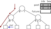
(a)

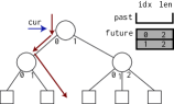
(b)

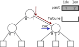
(c)

Figure 1. Several points in the execution of the replay-based nondeterminism algorithm.

When execution reaches a call to choose, it reads the choice to make from future, and pushes the result into the past. What if the future is unknown, as it will be in the first execution to reach a given call to choose? In this case, choose picks the first choice, and records it in past. Figure 1(c) depicts this scenario for the first time execution enters the else branch of our example.

⬇

NONE $\Rightarrow\;$ (* no future$\colon$ start a new index; push it into the past *)

let val i = start_idx xs in

push past i;

get xs i

end

$\mid$ SOME i $\Rightarrow\;$ (push past i;

get xs i)

The execution of a path in the computation tree ends when a value is returned. At this point, future is empty (all known choose calls have been executed), and past contains the complete path index. The withNondeterminism function is exactly the same as in Section 2.2, except that instead of updating the state to the next choice index, it computes the next path index, which becomes the future of the next run:

⬇

val next_future = List.rev (next_path (!past))

in

past := [];

future := next_future;

if !future = [] then v

else v @ withNondeterminism f

end

When withNondeterminism terminates, it must be the case that both (!past) = [] and (!future) = [], which allows to run it again.

⬇

val it = [1,2,3,4] $\colon$ int list

- withNondeterminism (fn () $\Rightarrow\;$ 2 + choose [1, 2, 3] * choose [1, 10, 100]);

val it = [3,12,102,4,22,202,5,32,302] $\colon$ int list

There is still one thing missing: doing nested calls to withNondeterminism would overwrite future and past, so nested calls return incorrect results.

⬇

else []);

val it = [[1,1,2]] $\colon$ int list list

2.4. Supporting nested calls

The final version of withNondeterminism supports nested calls by saving the current values of past and future onto a stack before each execution, and restoring them afterwards. No change to choose is needed.

⬇

fun withNondeterminism f =

(* before running, save current !past and !future value *)

(push nest (!past, !future);

past := [];

future := [];

let val result = loop f [] in

(* then restore them after the run *)

case pop nest of

NONE $\Rightarrow\;$ raise Impossible

$\mid$ SOME (p, f) $\Rightarrow\;$ (past := p;

future := f;

result))

end

and fun loop f acc =

(* by the way, let’s use a tail-recursive function *)

let val acc = ([f ()] handle Empty $\Rightarrow\;$ []) @ acc

val next_future = List.rev (next_path (!past))

in

past := [];

future := next_future;

if !future = [] then acc

else loop f acc

end

3. Continuations in Disguise

The previous section showed a trick for implementing direct-style nondeterminism in deterministic languages. Now, we delve to the deeper idea behind it, and surface the ability to generalize from nondeterminism to any monadic effect. We now examine how replay-based nondeterminism stealthily manipulates continuations. Consider evaluating this expression:

Every subexpression of e has a continuation, and when it returns a value, it invokes that continuation. After the algorithm takes e down the first path and reaches the point T = 2 * choose [5, 6], this second call to choose has continuation C = ($\square$  $\Rightarrow\;$ 2 * $\square$).

The choose function must invoke this continuation twice, with two different values. But C is not a function that can be repeatedly invoked: it’s a description of what the program does with a value after it’s returned, and returning a value causes the program to keep executing, consuming the continuation. So choose invokes this continuation the first time normally, returning $5$. To copy this ephemeral continuation, it re-runs the computation until it’s reached a point identical to T, evaluating that same call to choose with a second copy of C as its continuation — and this time, it invokes the continuation with $6$.

So, the first action of the choose operator is capturing the continuation. And what happens next? The continuation is invoked once for each value, and the results are later appended together. We’ve already seen another operation that invokes a function once on each value of a list and appends the results: the ListMonad.bind operator. Figure 2 depicts how applying ListMonad.bind to the continuation produces direct-style nondeterminism.

So, replay-based nondeterminism is actually a fusion of two separate ideas:

1. Capturing the continuation using replay

2. Using the captured continuation with operators from the nondeterminism monad

In Section 4, we extract the first half to create thermometer continuations, our replay-based implementation of delimited control. The second half — using continuations and monads to implement any effect in direct style — is Filinski’s construction, which we explain in Section 5. These produce something more inefficient than the replay-based nondeterminism of Section 2, but we’ll show in Section 6 how to fuse them together into something equivalent.

Figure 2. To implement choose: first capture the continuation, and then use the list monad’s bind operator to evaluate it multiple times.

4. Thermometer Continuations: Replay-Based Delimited Control

In the previous section, we explained how the replay-based nondeterminism algorithm actually hides a mechanism for capturing continuations. Over the the remainder of this section, we extract out that mechanism, developing the more general idea of thermometer continuations. But first, let us explain the variant of continuations that our mechanism uses: delimited continuations.

4.1. What is delimited control?

When we speak of "the rest of the computation," a natural question is "until where?" For traditional continuations, the answer is: until the program halts. This crosses all abstraction boundaries, making these "undelimited continuations" difficult to work with. Another answer is: until some programmer-specified "delimiter" or "reset point." This is the answer of delimited continuations, introduced by Felleisen, which only represent a prefix of the remaining computation. Just as call/cc makes continuations first class, allowing a program to modify its continuation to implement many different global control-flow operators, the shift and reset constructs make delimited continuations first-class, and can be used to implement many local control-flow operators.

In the remainder of this section, we’ll use the notation $E$[x] to denote plugging value $x$ into evaluation context $E$. We will also write $\square$(t) for the expression reset (fun () $\Rightarrow\;$ t). These notations makes it easy to give the semantics for shift and reset.

If the body of a reset reaches a value v, then this value is returned to the outside context.

On the other hand, if the evaluation inside a reset reaches a call to shift, then the argument of shift is invoked with a delimited continuation k corresponding to the entire evaluation context until the closest reset call:

where $E_{2}$ does not contain contexts of the form $\square$($E$). Figure 3 depicts this evaluation.

While call/cc captures an undelimited continuation that goes until the end of the program, shift only captures the continuation up to the first enclosing reset – it is delimited.

Notice that both the evaluation of shift’s argument t and the body of its continuation k are wrapped in their own reset calls; this affects the (quite delicate) semantics of nested calls to shift. There exists other variants of control operators that make different choices here.

If the continuation k passed to shift is never called, it means that the captured context $E_{2}$ is discarded and never used; this use of shift corresponds to exceptions.

⬇

$\Longrightarrow$ [3, 4]

On the other hand, using a single continuation multiple times can be used to emulate choose-style non-determinism.

⬇

$\Longrightarrow$ [6, 9, 12]

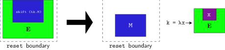
Figure 3. Graphical depiction of the action of the shift operator.

It is not easy to give precise polymorphic types to shift and reset; in this work, we make the simplifying assumption that they return a fixed “answer” type ans, as encoded in the following SML signature.

⬇

val reset $\colon$ (unit $\rightarrow$ ans) $\rightarrow$ ans

val shift $\colon$ (($\alpha$ $\rightarrow$ ans) $\rightarrow$ ans) $\rightarrow$ $\alpha$

end;

See the tutorial of Asai and Kiselyov for a more complete introduction to delimited control operators.

4.2. Baby Thermometer Continuations

Programming with continuations requires being able to capture and copy an intermediate state of the program. We showed in Section 3 that replay-based nondeterminism implicitly does this by replaying the whole computation, and hence needs no support from the runtime. We shall now see how to do this more explicitly.

This section presents a simplified version of thermometer continuations. This version assumes the reset block only contains one shift, which invokes its passed continuation $0$ or more times. It also restricts the body of shift and reset to only return integers. Still, this implementations makes it possible to handle several interesting examples.

Whenever we evaluate a reset, we’ll store its body as cur_expr:

⬇

fun reset f = (cur_expr := f;

(* rest of function given later *) )

Now, let $F$ be some function containing a single shift, i.e.: F = (fn () $\Rightarrow\;$ E[shift (fn k $\Rightarrow\;$ t))], where $E$ is a pure evaluation context (no additional effects). Then the main challenge in evaluating reset F is to capture the continuation of the shift as a function, i.e.: to obtain a C = (fn x $\Rightarrow\;$ E[x]).

Like the future stack in replay-nondeterminism that controls the action of choose, our trick is to use a piece of state to control shift.

Suppose we implement shift so that (state :=  SOME x; shift f) evaluates to x, regardless of f. Now consider a function which sets the state, and then replays the reset body, e.g.: a function k = (fn x $\Rightarrow\;$ (state :=  SOME x; (!cur_expr) ())). Because E is pure, the effectful code state :=  SOME x commutes with everything in E. This means the following equivalences hold:

⬇

$\equiv$ (state := SOME y; E[shift (fn k $\Rightarrow\;$ t)])

$\equiv$ E[state := SOME y; shift (fn k $\Rightarrow\;$ t)] (E commutes with state)

$\equiv$ E[y] (shift property)

which means that k is exactly the continuation we were looking for!

We are now ready to define reset and shift. reset sets the cur_expr to its body, and resets the state to NONE. It then runs its body. For the cases like reset (fn () $\Rightarrow\;$ 1 + shift (fn () $\Rightarrow\;$ 2)), where the shift aborts the computation and returns directly to reset, the shift will raise an exception and reset will catch it.

⬇

state := NONE;

(f () handle (Done x) $\Rightarrow\;$ x))

This gives us the definition of shift f: if shift f is being invoked from running the continuation, then state will not be NONE, and it should return the value in state. Else, it sets up a continuation as above, runs f with that continuation, and passes the result to the enclosing reset by raising an exception:

⬇

$\mid$ NONE $\Rightarrow\;$ let val expr = !cur_expr

fun k x = (state := SOME x;

expr ())

val result = f k

in

raise (Done result)

end

We can now evaluate some examples with basic delimited continuations:

⬇

- reset (fn () $\Rightarrow\;$ 1 + shift (fn k $\Rightarrow\;$ (k 1) * (k 2) * (k 3)))

val it = 24 $\colon$ int

The definitions given here lend themselves to a simple equational argument for correctness. Consider an arbitrary reset body with a single shift and no other effects. It reduces through these equivalences:

⬇

$\Longrightarrow$ $E_{1}$[$E_{2}$[raise (Done (let fun k x = (state := SOME x; $E_{2}$[shift (fn k $\Rightarrow\;$ t)]) in t))]

handle (Done x $\Rightarrow\;$ x)]

$\equiv$ $E_{1}$[let fun k x = (state := SOME x; $E_{2}$[shift (fn k $\Rightarrow\;$ t)]) in t]

$\equiv$ $E_{1}$[let fun k x = ($E_{2}$[state := SOME x; shift (fn k $\Rightarrow\;$ t)]) in t]

$\equiv$ $E_{1}$[let fun k x = ($E_{2}$[x]) in t]

Except for the nested reset’s, which do nothing in the case where there is only one shift, this is exactly the same as the semantics we gave in Section 4.1.

4.3. General Thermometer Continuations

Despite its simplicity, the restricted delimited control implementation of Section 4.2 already addressed the key challenge: capturing a continuation as a function. Just as we upgraded the single-choice nondeterminism into the full version, we’ll now upgrade that implementation into something that can handle arbitrary code with delimited continuations. We explain this process in five steps:

1. Allowing answer types other than int

2. Allowing multiple sequential shift’s

3. Allowing different calls to shift to return different types

4. Allowing nested shift’s

5. Allowing nested reset’s

We’ll go through each in sequence.

Different answer types

As mentioned in Section 4.1, it’s not easy to give precise polymorphic types to shift and reset. What can be done is to define them for any fixed answer type. An ML functor — a "function" that constructs modules — is used to parametrize over different answer types.

⬇

val cur_expr $\colon$ (unit $\rightarrow$ ans) ref = ref (fn () $\Rightarrow\;$ raise Impossible)

(* $\ldots$ all other definitions $\ldots$ *)

end;

Multiple sequential shift’s

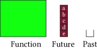
Figure 4. A thermometer continuation before being invoked

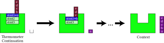
Figure 5. Graphical depiction of running a thermometer continuation

We will now generalize the construction of the previous section to multiple sequential shift’s. We do this similarly to what we did for replay nondeterminism, where we generalized the single choice index to a sequence of indices representing a path in the computation tree, and created the operation of sending execution along a certain path in the computation tree. This time, we generalize the simple state of the previous section which controls the return value of a shift, into a sequence of return values of sequential shift’s, making execution proceed in a certain fashion. Consider this example:

⬇

$\Longrightarrow$ 8

Suppose the state commands the first shift to return $x$ (call this Execution A). Then replaying the computation evaluates to x * shift (fn k’ $\Rightarrow\;$ 1 + k’ 3) — exactly the continuation of the first shift. Meanwhile, if the state commands the first shift to return $2$ (Execution B), and the second to return $x$, then replay will evaluate to 2 * x — this is the continuation of the second shift!

So, this state is a sequence of commands called frames, where each command instructs a shift to return a value (we’ll soon add another kind of command). The sequence of values to be returned by future calls to shift is called the future, so that Execution A was described by the future [RETURN x], and Execution B by [RETURN 2, RETURN x]. This means that the continuation could be described by everything up to the RETURN x, namely the empty list [] and [RETURN 2], respectively. This gives us our definition of a thermometer continuation:

Definition 4.1.

A thermometer continuation for a continuation $C$ is a pair of a list and a computation, $(s,\texttt{block})$, so that for appropriate change_state and run, the code change_state x s; run block evaluates to $C$[x].

Or, in code:

⬇

type thermo_cont = (unit $\rightarrow$ ans) * frame list

The key operation of thermometer continuations is to run the computation using the associated future, making execution proceed to a certain point. Just as in replay nondeterminism, during execution, each item is moved from the future to the past as it’s used:

⬇

val future $\colon$ frame list ref = ref []

Figure 4 depicts a thermometer continuation, while Figure 5 animates the execution of a thermometer continuation, showing how each value in the future matches with a shift, until the function being evaluated has the desired continuation. The left side of Figure 5 resembles a thermometer sticking out of the function, which inspired the name "thermometer continuations."

Different types for different shift’s

A future stores the values to be returned by different shift’s. When these shift’s are used at different types, the future will hence be a list of heterogeneous types, which poses typing problems. Replay-nondeterminism dodged this problem by storing an index into the choice list instead of the value to return itself. That solution does not work here, where the value to be returned may be from a distant part of the program. In an expression shift (fn k $\Rightarrow\;$ t), the continuation k will only be used to pass values to future invocations of that same shift, which has the correct type. However, we cannot explain this to the ML type system. Instead, we use a hack, a universal type u in which we assume that all types can be embedded and projected back:

⬇

val to_u $\colon$ $\alpha$ $\rightarrow$ u;

val from_u $\colon$ u $\rightarrow$ $\alpha$;

end;

structure Universal $\colon$ UNIVERSAL = struct

datatype u = U;

val to_u = Unsafe.cast;

val from_u = Unsafe.cast;

end;

We use this universal type to define the real frame type below.

Nested shift’s

With sequential shift’s, bringing execution to the desired point only required replacing shift’s with a return value. But with nested shift’s, the continuation to be captured may be inside another shift, and so replay will need to enter it. Consider this example:

⬇

val it = 37 $\colon$ int

The delimited continuation of the second shift is C = ($\square$  $\Rightarrow\;$ 3 * $\square$). In replay, execution must enter the body of the first shift, but replace the second shift with a value. So, in addition to RETURN frames, there must be another kind of frame, which instructs replay to enter the body of a shift.

Then, the desired computation is expressed simply as [ENTER], and can be evaluated with value x using the future [ENTER, RETURN x]. The values past and future are stacks of this frame type.

⬇

val future $\colon$ frame list ref = ref []

Nested reset’s

This is handled completely analogously to Section 2.4: each call to reset will push the previous state to a nesting stack, and restore it afterwards.

⬇

val nest $\colon$ reset_state list ref = ref []

We are now ready to begin giving the final implementation of thermometer continuations. As before, shift will pass its value to reset by raising an exception.

The key operation is to play a computation according to a known future. We implement this in the run_with_future function, which both does that, and establishes a new reset boundary. When doing so, it must save and restore the current state. This is similar to the withNondeterminism version with nesting, with the added management of cur_expr.

⬇

past := [];

future := f_future;

cur_expr := f;

let val result = (f () handle (Done x) $\Rightarrow\;$ x) in

case pop nest of

NONE $\Rightarrow\;$ raise Impossible

$\mid$ SOME (prev_expr, prev_past, prev_future) $\Rightarrow\;$

(cur_expr := prev_expr;

past := prev_past;

future := prev_future;

result)

end)

The reset we expose to the user is just a specialized instance of run_with_future, running with an empty future:

Finally, shift is similar to choose. The easy case is when the next item in the future is a return frame; it just has to return the commanded value.

⬇

(push past (RETURN v);

Universal.from_u v)

$\mid$ (NONE $\mid$ SOME ENTER) $\Rightarrow\;$

let val new_future = List.rev (!past)

val our_expr = !cur_expr

fun k v = run_with_future our_expr (new_future @ [RETURN (Universal.to_u v)])

val () = push past ENTER

val result = f k

in

raise (Done result)

end

The two other cases are more delicate. The ENTER case corresponds to the case where execution must enter the shift body — the function f. The case NONE is when the future is unknown, but, in that case, it should do exactly the same: enter the shift body.

It records this decision by pushing an ENTER frame into the past, and prepares a function k that invokes the thermometer continuation defined by (!cur_expr, List.rev (!past)). It invokes the thermometer continuation by appending a new value to the future, and then calling run_with_future. The body of the shift executes with this k; if it terminates normally, it raises an exception to pass the result to the enclosing reset.

⬇

$\Longrightarrow$ 37

4.4. What language features does this need?

Thermometer continuations clearly require exceptions and state, but the implementation of this section uses a couple other language features as well. Here, we discuss why we chose to use them, and ideas for alternatives.

Why we need  Unsafe.cast for universal types

Our implementation of thermometer continuations uses Unsafe.cast, as in the original presentation of Filinski, but shift and reset are carefully designed so that these casts never fail. Similarly, we believe that our use of Unsafe.cast is actually type-safe: we only inject values into the universal type at the call site of an effectful function, and only project values back in the same call site they are coming from.

In his follow-up paper, Filinski was able to upgrade these definitions to a type-safe implementation of the universal type. Unfortunately, we cannot just replace our implementation with a safe one.

Safe implementations of universal types cannot provide a pair of uniform polymorphic embedding and projection functions * (u $\rightarrow$ $\alpha$) – this is inherently unsafe. Instead, they provide a function that, on each call, generates a new embedding/projection pair for a given type: unit $\rightarrow$ (($\alpha$ $\rightarrow$ u) * (u $\rightarrow$ $\alpha$)). They all use a form of dynamic generativity, such as the allocation of new memory, or the creation of a new exception constructor.

These implementations do not work properly with our replay-based technique: each time a computation is replayed, a fresh embedding/projection pair is generated, and our implementation then tries to use the projection of a new pair on a value (of the same type) embedded by an old pair, which fails at runtime.

It may be possible to integrate the generation of universal embeddings within our replay machinery, to obtain safe implementations, but we left this delicate enhancement to future work.

Garbage Collection and Closures

This implementation uses closures heavily. This is a small barrier to someone implementing thermometer continuations in C, as they must encode all closures as function pointer/environment pairs. However, there’s a bigger problem: how to properly do memory management for these environments? A tempting idea is to release all environments after the last reset terminates, but this doesn’t work: the captured continuations may have unbounded lifetime, as exemplified by the state monad implementation in Section 5.4.

The options to solve this problem are the same as when designing other libraries with manual memory management: either make the library specialized enough that it can guess memory needs, or provide extra APIs so the programmer can indicate them. For example, one possibility for the latter is to allocate all closures for a given reset block in the same arena. At some point, the programmer knows that the code will no longer need any of the continuations captured within the reset. The programmer invokes an API to indicate this, and all memory in that arena is released.

5. Arbitrary Monads

In 1994, Filinski showed how to use delimited continuations to express any monadic effect in direct style. In this section, we hope to convey an intuition for Filinski’s construction, and also discuss what it looks like when combined with thermometer continuations. The code in this section comes almost verbatim from Filinski. This section is helpful for understanding the optimizations of Section 6, in which we explain how to fuse thermometer continuations with the code in this section.

5.1. Monadic Reflection

In SML and Java, there are two ways to program with mutable state. The first is to use the language’s built-in variables and assignment. The second is to use the monadic encoding, programming similar to how a pure language like Haskell handles mutable state. A stateful computation is a monadic value, a pure value of type $s\rightarrow(a,s)$.

These two approaches are interconvertible. A program can take a value of type $s\rightarrow(a,s)$ and run it, yielding a stateful computation of return type $a$. This operation is called reflect. Conversely, it can take a stateful computation of type $a$, and reify it into a pure value of type $s\rightarrow(a,s)$. Together, the reflect and reify operations give a correspondence between monadic values and effectful computations. This correspondence is termed monadic reflection. Fillinski showed how, using delimited control, it is possible to encode these operations as program terms.

The reflect and reify operations generalize to arbitrary monads. Consider nondeterminism, where a nondeterministic computation is either an effectful computation of type $\alpha$, or a monadic value of type $\alpha$ list. Then the reflect operator would take the input $[1,2,3]$ and nondeterministically return $1$, $2$, or $3$ — this is the choose operator from Section 2). So reify would take a computation that nondeterministically returns $1$, $2$, or $3$, and return the pure value $[1,2,3]$ — this is withNondeterminism.

So, for languages which natively support an effect, reflect and reify convert between effects implemented by the semantics of the language, and effects implemented within the language. Curry is a language with built-in nondeterminism, and it has these operators, calling them anyOf and getAllValues. SML does not have built-in nondeterminism, but, for our previous example, one can think of the code within a withNondeterminism block as running in a language extended with nondeterminism. So, one can think of the construction in the next section as being able to extend a language with any monadic effect.

In SML, monadic reflection is given by the following signature:

⬇

val reflect $\colon$ $\alpha$ M.m $\rightarrow$ $\alpha$

val reify $\colon$ (unit $\rightarrow$ $\alpha$) $\rightarrow$ $\alpha$ M.m

end;

5.2. Monadic Reflection through Delimited Control

Filinski’s insight was that the monadic style is similar to an older concept called continuation-passing style. We can see this by revisiting an example from Section 2. Consider this expression:

It is transformed into the monadic style as follows:

⬇

return (x * y)))

The first call to choose has continuation fn $\square$ $\Rightarrow\;$ $\square$ * (choose [5,6]). If x is the value returned by the first call to choose, the second has continuation fn $\square$ $\Rightarrow\;$ x * $\square$. These continuations correspond exactly to the functions bound in the monadic style. The monadic bind is the "glue" between a value and its continuation. Nondeterministically choosing from [2,3,4] wants to return thrice, which is the same as invoking the continuation thrice, which is the same as binding to the continuation.

So, converting a program to monadic style is quite similar to converting a program to this "continuation-passing style." Does this mean a language that has continuations can program with monads in direct style? Filinski answers yes.

The definition of monadic reflection in terms of delimited control is short. The overall setup is as follows:

⬇

structure M = M

fun reflect m = $\ldots$

fun reify t = $\ldots$

end;

Figure 2 showed how nondeterminism can be implemented by binding a value to the (delimited) continuation. The definition of reflect is a straightforward generalization of this.

If reflect uses shift, then reify uses reset to delimit the effects implemented through shift. This implementation requires use of type casts, because reset is monomorphized to return a value of type Universal.u m. Without these type casts, reify would read

Because of the casts, the actual definition of reify is slightly more complicated:

⬇

(M.return o Universal.from_u)

5.3. Example: Nondeterminism

Using this general construction, we immediately obtain an implementation of nondeterminism equivalent to the one in Section 2 by using ListMonad (defined in Section 2).

⬇

fun choose xs = N.reflect xs

fun fail () = choose []

- N.reify (fn () $\Rightarrow\;$ let val x = choose [2,3,4] * choose [5,7] in

if x $\geq$ 20 then x

else fail () end)

(* val it = [21,20,28] $\colon$ int list *)

It’s worth thinking about how this generic implementation executes on the example, and contrasting it with the direct implementation of Section 2. The direct implementation executes the function body $6$ times, once for each path of the computation. The generic one executes the function body $10$ times (once with a future stack of length $0$, $3$ times with length $1$, and $6$ times with length $2$). In the direct implementation, choose will return a value if it can. In the generic one, choose never returns. Instead, it invokes the thermometer continuation, causes the desired value to be returned at the equivalent point in the computation, and then raises an exception containing the final result. So, $4$ of those times, it could just return a value rather than replaying the computation. This is the idea of one of the optimizations we discuss in Section 6. This, plus one other optimization, let us derive the direct implementation from the generic one.

5.4. Example: State monad

State implemented through delimited control works differently from SML’s native support for state.

⬇

fun return x = fn s $\Rightarrow\;$ (x, s)

fun bind m f = fn s $\Rightarrow\;$ let val (x, s’) = m s

in f x s’ end

end;

structure S = Represent(StateMonad(type state = int))

fun tick () = S.reflect (fn s $\Rightarrow\;$ ((), s+1))

fun get () = S.reflect (fn s $\Rightarrow\;$ (s, s))

fun put n = S.reflect (fn _ $\Rightarrow\;$ ((), n))

- #1 (S.reify (fn () $\Rightarrow\;$ (put 5; tick ();

2 * get ()))

0)

(* val it = 12 $\colon$ int *)

Let’s take a look at how this works, starting with the example reify (fn () $\Rightarrow\;$ 3 * get ()).

⬇

$=$$\Rightarrow\;$ (reset (fn () $\Rightarrow\;$ return (3 * (shift (fn k $\Rightarrow\;$ bind (fn s $\Rightarrow\;$ (s, s)) k))))) 2

$=$$\Rightarrow\;$ (fn k $\Rightarrow\;$ bind (fn s $\Rightarrow\;$ (s,s)) k end)(fn x $\Rightarrow\;$ return (3*x)) 2

$=$$\Rightarrow\;$ (let val k = (fn x $\Rightarrow\;$ fn s $\Rightarrow\;$ (3*x, s)) in (fn s $\Rightarrow\;$ k s s)) 2

$=$$\Rightarrow\;$ (fn s $\Rightarrow\;$ (3*s, s)) 2

$=$$\Rightarrow\;$ (6, 2)

The get in reify (fn () $\Rightarrow\;$ 3 * get ()) suspends the current computation, causing the reify to return a function which awaits the initial state. Once invoked with an initial state, it resumes the computation (multiplying by $3$).

What does reify (fn () $\Rightarrow\;$ (tick (); get ())) do? The call to tick () again suspends the computation and awaits the state, as we can see from its expansion  shift (fn k $\Rightarrow\;$ fn s $\Rightarrow\;$ k () (s+1)). Once it receives s, it resumes it, returning () from tick. The call to get suspends the computation again, returning a function that awaits a new state; tick supplies s+1.

Think for a second about how this works when shift and reset are implemented as thermometer continuations. The get, put, and tick operators do not communicate by mutating state. They communicate by suspending the computation, i.e.: by raising exceptions containing functions. So, although the implementation of state in terms of thermometer continuations uses SML’s native support for state under the hood, it only does so tangentially, to capture the continuation.

6. Optimizations

Section 5.3 compared the two implementations of nondeterminism, and found that the generic one using thermometer continuations replayed the computation gratuitously. Thermometer continuations also replay the program in nested fashion, consuming stack space. In this section, we sketch a few optimizations that make monadic reflection via thermometer continuations less impractical, and illustrate the connections between the two implementations of nondeterminism.

All optimizations in this section save memoization require fusing thermometer continuations with monadic reflection. So, instead of using the definition of reflect in terms of shift given in Section 5.2, the require defining a single combined reflect operator.

6.1. CPS-bind: Invoking the Continuation at the Top of the Stack

The basic implementation of thermometer continuations wastes stack space. When there are multiple shift’s, execution will reach the first shift, then replay the function and reach the second shift, then replay again, etc, all the while letting the stack deepen. And yet, at the end, it will raise an exception that discards most of the computation on the stack. So, the implementation could save a lot of stack space by raising an exception before replaying the computation.

So, when a program invokes a thermometer continuation, it will need to raise an exception to transfer control to the enclosing reset, and thereby signal reset to replay the computation. While the existing Done exception signals that a computation is complete, it can do this with a second kind of exception, which we call Invoke.

However, the shift and reset functions do not invoke a thermometer continuation: the body of the shift does. In the case of monadic reflection, this is the monad’s bind operator. Raising an Invoke exception will discard the remainder of bind, so it must somehow also capture the continuation of bind. We can do this by writing bind itself in the continuation-passing style, i.e.: with the following signature:

⬇

val bind $\colon$ $\alpha$ m $\rightarrow$ ($\alpha$ $\rightarrow$ ($\beta$ m, $\gamma$) cont) $\rightarrow$ ($\beta$ m, $\gamma$) cont

The supplementary material contains code with this optimization, and uses it to implement nondeterminism in a way that executes more similarly to the direct implementation. We give here some key points. Here’s what the CPS’d bind operator for the list monad looks like:

⬇

$\mid$ bind (x$::$xs) f d = f x (fn a $\Rightarrow\;$ bind xs f (fn b $\Rightarrow\;$ d (a @ b)))

When used by reflect, f becomes a function that raises the Invoke exception, transferring control to the enclosing reset, which then replays the entire computation, but at the top level. The continuations of the bind get nested in a manner which is harder to describe, but ultimately get evaluated at the very end, also at the top level. So the list appends in d (a @ b) actually run at the top level of the reset, similar to how, in direct nondeterminism, it is the outer call to withNondeterminism that aggregates the results of each path.

While this CPS-monad optimization as described here can be used to implement many monadic effects, it cannot be used to implement all of them, nor general delimited continuations. Consider the state monad from Section 5.4: bind actually returns a function which escapes the outer reify. Then, when the program invokes that function and it tries to invoke its captured thermometer continuation, it will try to raise an Invoke exception to transfer control to its enclosing reify, but there is none. This CPS-monad optimization as described does not work if the captured continuation can escape the enclosing reset. With more work, it could use mutable state to track whether it is still inside a reset block, and then choose to raise an Invoke exception or invoke the thermometer continuation directly.

6.2. Direct Returns

In our implementation, a reset body E[reflect (return 1)] expands into

So, the entire computation up until that reflect runs twice. Instead of replaying the entire computation, that reflect could just return a value. E[reflect (return 1)] could expand into E[1].

The expression reflect (return 1) expands into shift (fn k $\Rightarrow\;$ bind (return 1) k). By the monad laws, this is equivalent to shift (fn k $\Rightarrow\;$ k 1). Tail-calling a continuation is the same as returning a value, so this is equivalent to 1. So, it’s the tail-call that allows this instance of reflect to return a value instead of replaying the computation.

Implementing the direct-return optimization is an additional small tweak to the CPS-bind optimization. We duplicate the second argument of bind, resulting in two function arguments that expect inputs at type $\alpha$.

To the implementor of bind, we ask that the first function be invoked on the first value of type $\alpha$ (if any) extracted out of the $\alpha$ m output, and the second be used on all later values.

In our implementation of reflect, we use this more flexible bind type for optimization. The second function argument we pass raises an Invoke exception, as described in Section 6.1. The first function returns a value directly, after updating the internal state of the thermometer. So, the first time bind invokes the continuation, it may do so by directly returning a value. Thereafter, it must invoke the continuation by explicitly raising an Invoke exception.

The bind operator for the list monad never performs a tail-call (it must always wrap the result in a list), but, after converting it to CPS, it always performs a tail-call. So this direct-return optimization combines well with the previous CPS-monad optimization. Indeed, applying them both transforms the generic nondeterminism of Section 5.3 into the direct nondeterminism of Section 2. In Section 7, we show benchmarks showing that this actually gives an implementation of nondeterminism as fast as the code in Section 2.

In the supplementary material, we demonstrate this optimization, providing optimized implementations of nondeterminism (list monad) and failure (maybe monad).

6.3. Memoization

While the frequent replays of thermometer continuations can interfere with any other effects in a computation, it cannot interfere with observationally-pure memoization. Memoizing nested calls to reset can save a lot of computation, and any expensive function can memoize itself without integrating into the implementation of thermometer continuations.

7. Performance numbers

The idea of invoking continuations by replaying the past at first seems woefully impractical. In fact, it performs surprisingly well in a diverse set of benchmarks. This shows that one may seriously consider using this approach to conveniently write non-performance-critical applications in a runtime (OCaml, Java, Javascript…) that does not provide control operators.

Working code for all benchmarks is available from https://github.com/jkoppel/thermometer-continuations.

7.1. The worst case

The overhead of replaying pure computations depends on the ratio, in an effectful program, of computation time spent in pure and impure computations, and in the branching structure of the computation tree.

The worst case is when a program runs a costly pure computation, followed by large branching of an effect – causing many replays. The overhead may be arbitrarily large; for example, replay-based or thermometer-based implementations cause a 10x slowdown on the following program:

⬇

val i = choose [0,1,2,3,4,5,6,7,8,9] in

(i, v)

end

)

7.2. Search-heavy programs: N-queens

Table 1. Benchmark NQUEENS

OCaml times	10	11	12	13
Indirect	0.007s	0.037s	0.213s	1.308s
Replay	0.017s	0.101s	0.597s	3.768s
Therm.	0.041s	0.221s	1.347s	8.621s
Therm. Opt.	0.019s	0.111s	0.65s	3.924s
Filinski (Delimcc)	0.035s	0.185s	1.236s	14.412s
Eff. Handlers (Multicore OCaml)	0.019s	0.092s	0.509s	2.81s

SML times 10 11 12 13 Indirect 0.011s 0.064s 0.36s 2.166s Replay 0.029s 0.164s 1.051s 6.562s Therm. 0.06s 0.344s 2.152s 14.305s Therm. Opt. 0.03s 0.173s 1.151s 6.793s Filinski (Call/cc) 0.015s 0.079s 0.493s 2.941s MLton times 10 11 12 13 Indirect 0.007s 0.031s 0.187s 1.129s Replay 0.016s 0.099s 0.637s 4.295s Finlinski (Call/cc) 0.078s 0.399s 2.138s 12.62s Prolog times 10 11 12 13 Prolog search (GNU Prolog) 0.165s 0.614s 3.307s 20.401s

The benchmark NQUEENS is the problem of enumerating all solutions to the n-queens problem. It is representative of search programs where most of the time is spent in backtracking search, and we decided to test our approach against a wide variety of alternative implementations to get a sense of the replay overhead on search-heavy non-deterministic programs. Table 7.2 reports the times for each implementation for different $n$.

Numbers in this section were collected using SML/NJ v110.82, OCaml 4.06, MLton 2018-02-07, the experimental OCaml-multicore runtime for OCaml 4.02.2 (dev0), and GNU Prolog 1.4.4, on a Lenovo T440s with an 1.6GHz Intel Core i5 processor.

All implementations are exponential, and the slope (the exponential coefficient) is essentially the same for all implementations: for a given node in the computation tree, the overhead of replaying the past is proportional to its depth, which is bounded by $n$, and this bounded multiplicative slowdown factor becomes a $log(n)$ additive overhead in log-scale.

The generic thermometer-based implementation (using Filinski’s construction with replay-based shift and reset) is noticeably slower than the simpler replay-based implementation of non-determinism. On the other hand, the optimizations described in Section 6 suffice to remove the additional overhead: optimized thermometers are just as fast as replay-nondeterminism.

We benchmarked Filinski’s construction using the delimcc library, which is an implementation of delimited control doing low-level stack copying; it is comparable in speed to the generic thermometers. This is a nice result even though delimcc is known not to be competitive with control operators in runtimes designed to make them efficient.

We also wrote a version of the benchmark using the effect handlers provided by the experimental Multicore OCaml runtime. The performance is better than our replay-based non-determinism (or optimized thermometers), but in the same logarithmic ballpark.

In contrast, in our SML benchmarks, Filinski’s construction using the native call/cc of SML/NJ is significantly faster than replay-based approaches, closer to the indirect-style baseline. We explain this by the fact that the SML/NJ compilation strategy and runtime has made choices (call frames on the heap) that give a very efficient call/cc, but add some overhead (compared to using the native stack) to general computation. Indeed, in absolute time, OCaml’s indirect baseline is about 60$\%$ faster than the SML/NJ baseline, and SML/NJ’s call/cc approach is actually only 30$\%$ faster than OCaml’s best replay-based implementations, and slower than the Multicore-OCaml implementation.

To validate this hypothesis, we measured the performance of MLton on the benchmarks that it supports (not thermometers, which require a working Unsafe.cast; see Section 4.4). The performance results for the indirect and replay-nondeterminism version are extremely similar to OCaml’s, but the call/cc version is much slower than the one of SML/NJ, similar to the performances of delim/cc; on MLton, our replay-based technique is the best direct-style implementation of non-determinism.

Finally, we wrote a Prolog version of N-queens (using Prolog’s direct-style backtracking search, not constraint solving). We were surprised to find out that it is slower than all other implementations. For N=13, GNU Prolog takes around 20s, while our slowest ML versions run in 14s. Prolog may have efficient support for backtracking search, but it seems disadvantaged by being a dynamically-typed language without an aggressive JIT implementation.

Our conclusion is that for computations dominated by nondeterministic search, replay-based approaches are surprisingly practical: they offer reasonable performances compared to other approaches to direct-style nondeterminism that are considered practical.

7.3. More benchmarks

More benchmarks in different monads are included in Appendix B.

8. But Isn’t This Impossible?

In a 1990 paper, Matthias Felleisen presented formal notions of expressibility and macro-expressibility of one language feature in terms of others, along with proof techniques to show a feature cannot be expressed. Hayo Thielecke used these to show that exceptions and state together cannot macro-express continuations. This is concerning, because, at first glance, this is exactly what we did.

First, a quick review of Felleisen’s concepts: Expressibility and macro-expressibility help define what should be considered core to a language, and what is mere "syntactic sugar." An expression is a translation from a language $\mathcal{L}$ containing a feature $\mathcal{F}$ to a language $\mathcal{L}^{\prime}$ without it which preserves program semantics. A key restriction is that an expression may only rewrite AST nodes that implement $\mathcal{F}$ and the descendants of these nodes. So, an expression of state may only rewrite assignments, dereferences, and expressions that allocate reference cells. Whle there is a whole-program transformation that turns stateful programs into pure programs, namely by threading a "state" variable throughout the entire program, this transformation is not an expression. A macro-expression is an expression which may rewrite nodes from $\mathcal{F}$, but may only move or copy the children of such nodes (technically speaking, it must be a term homomorphism). A classic example of a macro-expression is implementing the += operator in terms of normal assignment and addition. A classic example of an expression which is not a macro-expression is desugaring for-loops into while-loops (it must dig into the loop body and modify every continue statement). Another one is implementing Java finally blocks (which need to execute an action after every return statement).

It turns out that Thielecke’s proof does not immediately apply. First, it concerns call/cc-style continuations rather than delimited continuations. This seems like a minor limitation, since delimited continuations can be use to implement call/cc. But the second reason is more fundamental.

Thielecke’s proof is based on showing that, in a language with exceptions and state but not continuations, all expressions of the following form with different $j$ are operationally equivalent:

$$R_{j}=\lambda f.((\lambda x.\lambda y.(f\;0;\;x:=\;!y;y:=j;!x))(\text{ref}\;0)(\text{ref}\;0))$$

The intuition behind this equivalence is that the two reference cells are allocated locally and then discarded, and so the value stored in them can never be observed. However, with continuations, on the other hand, $f$ could cause the two assignments to run twice on the same reference cells.

This example breaks down because it cannot be expressed in our monadic reflection framework as is. The monadic reflection framework assumes there are no other effects within the program other than the ones implemented via monadic reflection. To write the $R_{j}$ using thermometer continuations and monadic reflection, the uses of ref must be changed from the native SML version to one implemented using the state monad. Then, when the computation is replayed, repeated calls to ref may return the same reference cell, allowing the state to escape, thereby allowing different $R_{j}$ to be distinguished. What this means is, because thermometer continuations require rewriting uses of mutable state, and not only uses of shift and reset, they are not a macro-expression. So, Thielecke’s theorem does not apply.

9. Related Work

Our work is most heavily based on Filinski’s work expressing monads using delimited control. We have also discussed theoretical results regarding the inter-expressibility of exceptions and continuations in Section 8. Other work on implementing continuations using exceptions relate the two from a runtime-engineering perspective and from a typing perspective.

Continuations from stack inspection

Oleg Kiselyov’s delimcc library provides an implementation of delimited control for OCaml, based on the insight that the stack-unwinding facilities used to implement exceptions are also useful in implementing delimited control. Unlike our approach, delimcc works by tightly integrating with the OCaml runtime, exposing low-level details of its virtual machine to user code. Its implementation relies on copying portions of the stack into a data structure, repurposing functionality used for recovering from stack overflows. It hence would not work for e.g.: many implementations of Java, which recover from stack overflows by simply deleting activation records. On the other hand, its low-level implementation makes it efficient and lets it persist delimited continuations to disk. A similar insight is used by Pettyjohn et al to implement continuations using a global program transformation.

Replay-based web programming

WASH Server Pages is a web framework that uses replay to persist state across multiple requests. In WASH, a single function can both display an HTML form to the end user, and take an action based on the user’s response: the function is run twice, with the user’s response stored in a replay log. MFlow , another web framework, works along similar principles. Our work shows how the replay logs used by these frameworks are equivalent to serializing a continuation, revealing the connection between MFlow/WASH and continuation-based web frameworks.

Typing power of exceptions vs. continuations

Lillibridge shows that exceptions introduce a typing loophole that can be used to implement unbounded loops in otherwise strongly-normalizing languages, while continuations cannot do this, giving the slogan "Exceptions are strictly more powerful than call/cc." As noted by other authors, this argument only concerns the typing of exceptions rather than their execution semantics, and is inapplicable in languages that already have recursion.

10. Conclusion

Filinski’s original construction of monadic reflection from delimited continuations, and delimited continuations from normal continuations plus state, provided a new way to program for the small fraction of languages which support first-class continuations. With our demonstration that exceptions and state are sufficient, this capability is extended to a large number of popular languages, including 9 of the TIOBE 10 (all but C). While languages like Haskell with syntactic support for monads may not benefit from this construction, bringing advanced monadic effects to more languages paves the way for ideas spawned in the functional programming community to influence a broader population.

In fact, the roots of this paper came from an attempt to make one of the benefits of monads more accessible. We built a framework for Java where a user could write something that looks like a normal interpreter for a language, but, executed differently, it would become a flow-graph generator, a static analyzer, a compiler, etc. Darais showed that this could be done by writing an interpreter in the monadic style (concrete interpreters run programs directly; abstract interpreters run them nondeterministically). We discovered this concurrently with Darais, and then discovered replay-based nondeterminism so that Java programmers could write normal, non-monadic programs.

Despite the apparent inefficiency of thermometer continuations, the surprisingly good performance results of Section 7, combined with the oft-unused speed of modern machines, provide hope that the ideas of this paper can find their way into practical applications. Indeed, Filinski’s construction is actually known as a way to make programs faster.

Overall, we view finding a way to bring delimited control into mainstream languages as a significant achievement. We hope to see a flourishing of work with advanced effects now that they can be used by more programmers.

Working code for all examples and benchmarks, as well as the CPS-bind and direct-return optimizations, is available from https://github.com/jkoppel/thermometer-continuations .

Appendix A Is this possibly correct?

In this section, we provide a correctness proof of our construction in the simplest possible case: the replay-based implementation of non-deterministic computations with a two-argument choose x y effect, in a simplistic toy language.

We consider programs with the following grammar. Notice that, for simplicity, we only allow our choice operator $\mathsf{choose}~{}x~{}y$ to take variables as parameters, rather than arbitrary expressions.

$$\begin{array}[]{l@{~}r@{~}l@{\quad}l}t,u\hfil~{}&\mathrel{\mathord{:}\mathord{:=}}~{}&&\mbox{terms}\\ \hfil~{}&\mid~{}&x,y,z...&\mbox{variables}\\ \hfil~{}&\mid~{}&n\in\mathbb{N}&\mbox{number constant}\\ \hfil~{}&\mid~{}&\mathsf{S}~{}t&\mbox{successor}\\ \hfil~{}&\mid~{}&\mathsf{let}~{}x\,=\,t~{}\mathsf{in}~{}u&\mbox{let-binding}\\ \hfil~{}&\mid~{}&\mathsf{choose}~{}x~{}y&\mbox{choice}\\ \end{array}$$

To make the execution semantics of non-deterministic choice precise, we define a notion of abstract machine, the continuation machines. Continuation machines are quadruples $(t,{\color[rgb]{0,0,1}K},{\color[rgb]{0,0,1}s},R)$ of a term, a current machine continuation ${\color[rgb]{0,0,1}K}$, a soup of threads ${\color[rgb]{0,0,1}s}$ that are waiting to execute next, and a result $R$, which is a list of integers. Machine continuations are given by the following very simple grammar, and thread soups ${\color[rgb]{0,0,1}s}$ are lists of pairs $(t,{\color[rgb]{0,0,1}K})$ of a term and a continuation.

$$\begin{array}[]{l@{~}r@{~}l@{\quad}l}{\color[rgb]{0,0,1}K}\hfil~{}&\mathrel{\mathord{:}\mathord{:=}}~{}&&\mbox{machine stacks}\\ \hfil~{}&\mid~{}&{\color[rgb]{0,0,1}\mathsf{S}~{}{\color[rgb]{0,0,1}K}}&\mbox{successor}\\ \hfil~{}&\mid~{}&{\color[rgb]{0,0,1}\mathsf{let}~{}{\color[rgb]{0,0,0}x}\,=\,\square~{}\mathsf{in}~{}({\color[rgb]{0,0,0}t},{\color[rgb]{0,0,1}K})}&\mbox{binding}\\ \hfil~{}&\mid~{}&{\color[rgb]{0,0,1}\mathsf{halt}}&\mbox{halt instruction}\\ \end{array}\qquad\begin{array}[]{l}{\color[rgb]{0,0,1}s}\quad\mathrel{\mathord{:}\mathord{:=}}\quad\emptyset\;\mid\;(t,{\color[rgb]{0,0,1}K}).{\color[rgb]{0,0,1}s}\\ R\quad\mathrel{\mathord{:}\mathord{:=}}\quad\emptyset\;\mid\;n.R\\ \end{array}$$

We can now define a reduction relation $(t,{\color[rgb]{0,0,1}K},{\color[rgb]{0,0,1}s^{\prime}},R)\mathrel{{\color[rgb]{0,0,1}\rightarrow}}(t^{\prime},{\color[rgb]{0,0,1}K^{\prime}},{\color[rgb]{0,0,1}s^{\prime}},R^{\prime})$ to formally define the execution of those non-deterministic programs. If $(t,{\color[rgb]{0,0,1}\mathsf{halt}},\emptyset,\emptyset)$ eventually reduces to $(n,{\color[rgb]{0,0,1}\mathsf{halt}},\emptyset,R)$ for $n\in\mathbb{N}$, then the meaning of the program is the result $n.R$. $\displaystyle\begin{array}[]{l@{\quad\contrew\quad}l}({\color[rgb]{0,0,0}\mathsf{S}~{}{\color[rgb]{0,0,0}t}},{\color[rgb]{0,0,1}K},{\color[rgb]{0,0,1}s},R)\hfil\quad\mathrel{{\color[rgb]{0,0,1}\rightarrow}}&(t,{\color[rgb]{0,0,1}\mathsf{S}~{}{\color[rgb]{0,0,1}K}},{\color[rgb]{0,0,1}s},R)\\ (n,{\color[rgb]{0,0,1}\mathsf{S}~{}{\color[rgb]{0,0,1}K}},{\color[rgb]{0,0,1}s},R)\hfil\quad\mathrel{{\color[rgb]{0,0,1}\rightarrow}}&(n+1,{\color[rgb]{0,0,1}K},{\color[rgb]{0,0,1}s},R)\\ \penalty 50\hskip 20.00003pt plus 0.5fil minus 5.0pt({\color[rgb]{0,0,0}\mathsf{let}~{}{\color[rgb]{0,0,0}x}\,=\,{\color[rgb]{0,0,0}t}~{}\mathsf{in}~{}{\color[rgb]{0,0,0}u}},{\color[rgb]{0,0,1}K},{\color[rgb]{0,0,1}s},R)\hfil\quad\mathrel{{\color[rgb]{0,0,1}\rightarrow}}&(t,{\color[rgb]{0,0,1}\mathsf{let}~{}{\color[rgb]{0,0,0}x}\,=\,\square~{}\mathsf{in}~{}({\color[rgb]{0,0,0}u},{\color[rgb]{0,0,1}K})},{\color[rgb]{0,0,1}s},R)\\ (n,{\color[rgb]{0,0,1}\mathsf{let}~{}{\color[rgb]{0,0,0}x}\,=\,\square~{}\mathsf{in}~{}({\color[rgb]{0,0,0}u},{\color[rgb]{0,0,1}K})},{\color[rgb]{0,0,1}s},R)\hfil\quad\mathrel{{\color[rgb]{0,0,1}\rightarrow}}&(u[x\leftarrow n],{\color[rgb]{0,0,1}K},{\color[rgb]{0,0,1}s},R)\\ \end{array}\penalty 50\hskip 20.00003pt plus 0.5fil minus 5.0pt\begin{array}[]{l@{\quad\contrew\quad}l}(\mathsf{choose}~{}n_{1}~{}n_{2},{\color[rgb]{0,0,1}K},{\color[rgb]{0,0,1}s},R)\hfil\quad\mathrel{{\color[rgb]{0,0,1}\rightarrow}}&(n_{1},{\color[rgb]{0,0,1}K},(n_{2},{\color[rgb]{0,0,1}K}).{\color[rgb]{0,0,1}s},R)\\ \penalty 50\hskip 20.00003pt plus 0.5fil minus 5.0pt(n,{\color[rgb]{0,0,1}\mathsf{halt}},(n^{\prime},{\color[rgb]{0,0,1}K}).{\color[rgb]{0,0,1}s},R)\hfil\quad\mathrel{{\color[rgb]{0,0,1}\rightarrow}}&(n^{\prime},{\color[rgb]{0,0,1}K},{\color[rgb]{0,0,1}s},n.R)\\ \end{array}$ The two last rules give the semantics of parallelism: $\mathsf{choose}~{}n_{1}~{}n_{2}$ returns $n_{1}$, but adds the thread $(n_{2},{\color[rgb]{0,0,1}K})$ to the soup, to be executed later, and the ${\color[rgb]{0,0,1}\mathsf{halt}}$ rule adds a number to the result set and restarts the next thread in the soup. Note that the rule for $\mathsf{choose}~{}n_{1}~{}n_{2}$ duplicates the continuation ${\color[rgb]{0,0,1}K}$, pushing a copy of it on the thread soup: this machine relies on a runtime that can duplicate continuations.

Our correctness argument comes from defining an alternative notion of abstract machines for these programs, the history machines, that model our replay-based technique. History machines are of the form $(t,{\color[rgb]{0,0,1}K},{\color[rgb]{1,0,0}P},{\color[rgb]{1,0,0}F},R)_{u}$, replacing the soup ${\color[rgb]{0,0,1}s}$ with a past ${\color[rgb]{1,0,0}P}$ and a future ${\color[rgb]{1,0,0}F}$ which are just ordered lists of choices ${\color[rgb]{1,0,0}i}$ – numbers in $\{1,2\}$. Finally, $u$ is the initial computation that gets replayed; it is constant over the whole execution. We also define an operation $P{\color[rgb]{1,0,0}+1}$ corresponding to the next_path function of Section 2.3, which gets stuck on an empty path: $\emptyset{\color[rgb]{1,0,0}+1}$ is just $\emptyset{\color[rgb]{1,0,0}+1}$. $\displaystyle\begin{array}[]{l@{\quad\gramdef\quad}l}{\color[rgb]{1,0,0}i}\hfil\quad\mathrel{\mathord{:}\mathord{:=}}&1\mid 2\\ \end{array}\penalty 50\hskip 20.00003pt plus 0.5fil minus 5.0pt\begin{array}[]{l@{\quad\gramdef\quad}l}{\color[rgb]{1,0,0}P}\hfil\quad\mathrel{\mathord{:}\mathord{:=}}&\emptyset\mid{\color[rgb]{1,0,0}P}.{\color[rgb]{1,0,0}i}\\ {\color[rgb]{1,0,0}F}\hfil\quad\mathrel{\mathord{:}\mathord{:=}}&\emptyset\mid{\color[rgb]{1,0,0}i}.{\color[rgb]{1,0,0}F}\\ \end{array}\penalty 50\hskip 20.00003pt plus 0.5fil minus 5.0pt\begin{array}[]{l@{\quad\eqdef\quad}l}{\color[rgb]{1,0,0}P}.{\color[rgb]{1,0,0}1}{\color[rgb]{1,0,0}+1}\hfil\quad\stackrel{{\scriptstyle\mathsf{def}}}{{=}}&{\color[rgb]{1,0,0}P}.2\\ {\color[rgb]{1,0,0}P}.{\color[rgb]{1,0,0}2}{\color[rgb]{1,0,0}+1}\hfil\quad\stackrel{{\scriptstyle\mathsf{def}}}{{=}}&{\color[rgb]{1,0,0}P}{\color[rgb]{1,0,0}+1}\\ \end{array}\penalty-10000\hskip 20.00003pt plus 0.5fil minus 5.0pt\begin{array}[]{l@{\;\histrew\;}l}({\color[rgb]{0,0,0}\mathsf{S}~{}{\color[rgb]{0,0,0}t}},{\color[rgb]{0,0,1}K},{\color[rgb]{1,0,0}P},{\color[rgb]{1,0,0}F},R)_{u}\hfil\;\mathrel{{\color[rgb]{1,0,0}\to}}&(t,{\color[rgb]{0,0,1}\mathsf{S}~{}{\color[rgb]{0,0,1}K}},{\color[rgb]{1,0,0}P},{\color[rgb]{1,0,0}F},R)_{u}\\ (n,{\color[rgb]{0,0,1}\mathsf{S}~{}{\color[rgb]{0,0,1}K}},{\color[rgb]{1,0,0}P},{\color[rgb]{1,0,0}F},R)_{u}\hfil\;\mathrel{{\color[rgb]{1,0,0}\to}}&(n+1,{\color[rgb]{0,0,1}K},{\color[rgb]{1,0,0}P},{\color[rgb]{1,0,0}F},R)_{u}\\ \penalty 50\hskip 20.00003pt plus 0.5fil minus 5.0pt({\color[rgb]{0,0,0}\mathsf{let}~{}{\color[rgb]{0,0,0}x}\,=\,{\color[rgb]{0,0,0}t}~{}\mathsf{in}~{}{\color[rgb]{0,0,0}t^{\prime}}},{\color[rgb]{0,0,1}K},{\color[rgb]{1,0,0}P},{\color[rgb]{1,0,0}F},R)_{u}\hfil\;\mathrel{{\color[rgb]{1,0,0}\to}}&(t,{\color[rgb]{0,0,1}\mathsf{let}~{}{\color[rgb]{0,0,0}x}\,=\,\square~{}\mathsf{in}~{}({\color[rgb]{0,0,0}t^{\prime}},{\color[rgb]{0,0,1}K})},{\color[rgb]{1,0,0}P},{\color[rgb]{1,0,0}F},R)_{u}\\ (n,{\color[rgb]{0,0,1}\mathsf{let}~{}{\color[rgb]{0,0,0}x}\,=\,\square~{}\mathsf{in}~{}({\color[rgb]{0,0,0}t^{\prime}},{\color[rgb]{0,0,1}K})},{\color[rgb]{1,0,0}P},{\color[rgb]{1,0,0}F},R)_{u}\hfil\;\mathrel{{\color[rgb]{1,0,0}\to}}&(t^{\prime}[x\leftarrow n],{\color[rgb]{0,0,1}K},{\color[rgb]{1,0,0}P},{\color[rgb]{1,0,0}F},R)_{u}\\ \end{array}\penalty 50\hskip 20.00003pt plus 0.5fil minus 5.0pt\begin{array}[]{l@{\quad\histrew\quad}l}(\mathsf{choose}~{}n_{1}~{}n_{2},{\color[rgb]{0,0,1}K},{\color[rgb]{1,0,0}P},\emptyset,R)_{u}\hfil\quad\mathrel{{\color[rgb]{1,0,0}\to}}&(\mathsf{choose}~{}n_{1}~{}n_{2},{\color[rgb]{0,0,1}K},{\color[rgb]{1,0,0}P},1.\emptyset,R)_{u}\\ \penalty 50\hskip 20.00003pt plus 0.5fil minus 5.0pt(\mathsf{choose}~{}n_{1}~{}n_{2},{\color[rgb]{0,0,1}K},{\color[rgb]{1,0,0}P},({\color[rgb]{1,0,0}i}.{\color[rgb]{1,0,0}F}),R)_{u}\hfil\quad\mathrel{{\color[rgb]{1,0,0}\to}}&(n_{{\color[rgb]{1,0,0}i}},{\color[rgb]{0,0,1}K},({\color[rgb]{1,0,0}P}.{\color[rgb]{1,0,0}i}),{\color[rgb]{1,0,0}F},R)_{u}\\ \penalty 50\hskip 20.00003pt plus 0.5fil minus 5.0pt(n,{\color[rgb]{0,0,1}\mathsf{halt}},{\color[rgb]{1,0,0}P},\emptyset,R)_{u}\hfil\quad\mathrel{{\color[rgb]{1,0,0}\to}}&(u,{\color[rgb]{0,0,1}\mathsf{halt}},\emptyset,{\color[rgb]{1,0,0}P}{\color[rgb]{1,0,0}+1},n.R)_{u}\\ \end{array}$ When we reach an instruction $\mathsf{choose}~{}n_{1}~{}n_{2}$, the machine picks the value $n_{{\color[rgb]{1,0,0}i}}$ (for ${\color[rgb]{1,0,0}i}\in\{1,2\}$) determined by its future ${\color[rgb]{1,0,0}F}$. When it finishes computing a value $n$ with past history ${\color[rgb]{1,0,0}P}$, it restarts the whole computation $u$ with future ${\color[rgb]{1,0,0}P}{\color[rgb]{1,0,0}+1}$, exactly like our implementation. The semantics of a term $t$ for these machines is given by the result $R$ such that $(t,{\color[rgb]{0,0,1}\mathsf{halt}},\emptyset,\emptyset,\emptyset)_{t}$ reduces to $(t,{\color[rgb]{0,0,1}\mathsf{halt}},\emptyset,\emptyset{\color[rgb]{1,0,0}+1},R)_{t}$.

Remarkably, this machine never duplicates a continuation ${\color[rgb]{0,0,1}K}$; it can be implemented in language lacking this runtime capability. It is also interesting to compare how ${\color[rgb]{0,0,1}K}$ and $({\color[rgb]{1,0,0}P},{\color[rgb]{1,0,0}F})$ grow over time: ${\color[rgb]{0,0,1}K}$ grows at each reduction, including of non-effectful operations, while $({\color[rgb]{1,0,0}P},{\color[rgb]{1,0,0}F})$ only changes at the call sites of $\mathsf{choose}~{}n_{1}~{}n_{2}$ and on ${\color[rgb]{0,0,1}\mathsf{halt}}$ – it only records the effects in the computation tree. Tracking the value of ${\color[rgb]{0,0,1}K}$ in user code would require inserting code around all operations, while $({\color[rgb]{1,0,0}P},{\color[rgb]{1,0,0}F})$ can be tracked by clever implementations of the effectful operators only.

Correctness of the history machine means that the second reduction semantics produces the same results as the first one. One way to do this is to convince ourselves that the reductions of both machine embed in the following combined machines, where machine continuations ${\color[rgb]{0,0,1}K}$ are annotated with a past ${\color[rgb]{1,0,0}P}$ – including in the soup – and the machine also holds a future ${\color[rgb]{1,0,0}F}$:

$\displaystyle\begin{array}[]{l@{\;\to\;}l}({\color[rgb]{0,0,0}\mathsf{S}~{}{\color[rgb]{0,0,0}t}},{{\color[rgb]{0,0,1}K}}_{{\color[rgb]{1,0,0}P}},{\color[rgb]{1,0,0}F},{\color[rgb]{0,0,1}s},R)_{u}&(t,{({\color[rgb]{0,0,1}\mathsf{S}~{}{\color[rgb]{0,0,1}K}})}_{{\color[rgb]{1,0,0}P}},{\color[rgb]{1,0,0}F},{\color[rgb]{0,0,1}s},R)_{u}\\ (n,{({\color[rgb]{0,0,1}\mathsf{S}~{}{\color[rgb]{0,0,1}K}})}_{{\color[rgb]{1,0,0}P}},{\color[rgb]{1,0,0}F},{\color[rgb]{0,0,1}s},R)_{u}&(n+1,{{\color[rgb]{0,0,1}K}}_{{\color[rgb]{1,0,0}P}},{\color[rgb]{1,0,0}F},{\color[rgb]{0,0,1}s},R)_{u}\\ \penalty 50\hskip 20.00003pt plus 0.5fil minus 5.0pt({\color[rgb]{0,0,0}\mathsf{let}~{}{\color[rgb]{0,0,0}x}\,=\,{\color[rgb]{0,0,0}t}~{}\mathsf{in}~{}{\color[rgb]{0,0,0}t^{\prime}}},{{\color[rgb]{0,0,1}K}}_{{\color[rgb]{1,0,0}P}},{\color[rgb]{1,0,0}F},{\color[rgb]{0,0,1}s},R)_{u}&(t,{({\color[rgb]{0,0,1}\mathsf{let}~{}{\color[rgb]{0,0,0}x}\,=\,\square~{}\mathsf{in}~{}({\color[rgb]{0,0,0}t^{\prime}},{\color[rgb]{0,0,1}K})})}_{{\color[rgb]{1,0,0}P}},{\color[rgb]{1,0,0}F},{\color[rgb]{0,0,1}s},R)_{u}\\ (n,{({\color[rgb]{0,0,1}\mathsf{let}~{}{\color[rgb]{0,0,0}x}\,=\,\square~{}\mathsf{in}~{}({\color[rgb]{0,0,0}t^{\prime}},{\color[rgb]{0,0,1}K})})}_{{\color[rgb]{1,0,0}P}},{\color[rgb]{1,0,0}F},{\color[rgb]{0,0,1}s},R)_{u}&(t^{\prime}[x\leftarrow n],{{\color[rgb]{0,0,1}K}}_{{\color[rgb]{1,0,0}P}},{\color[rgb]{1,0,0}F},{\color[rgb]{0,0,1}s},R)_{u}\\ \end{array}\penalty 50\hskip 20.00003pt plus 0.5fil minus 5.0pt\begin{array}[]{l@{\quad\to\quad}l}(\mathsf{choose}~{}n_{1}~{}n_{2},{{\color[rgb]{0,0,1}K}}_{{\color[rgb]{1,0,0}P}},\emptyset,{\color[rgb]{0,0,1}s},R)_{u}&(n_{1},{{\color[rgb]{0,0,1}K}}_{{\color[rgb]{1,0,0}P}.{\color[rgb]{1,0,0}1}},\emptyset,(n_{2},{\color[rgb]{0,0,1}K}_{{\color[rgb]{1,0,0}P}.{\color[rgb]{1,0,0}2}}).{\color[rgb]{0,0,1}s},R)_{u}\\ \penalty 50\hskip 20.00003pt plus 0.5fil minus 5.0pt(n,{{\color[rgb]{0,0,1}\mathsf{halt}}}_{{\color[rgb]{1,0,0}P}},\emptyset,(n^{\prime},{\color[rgb]{0,0,1}K}_{{\color[rgb]{1,0,0}P^{\prime}}}).{\color[rgb]{0,0,1}s},R)_{u}&(n^{\prime},{{\color[rgb]{0,0,1}K}}_{{\color[rgb]{1,0,0}P^{\prime}}},\emptyset,{\color[rgb]{0,0,1}s},n.R)_{u}\\ \penalty 50\hskip 20.00003pt plus 0.5fil minus 5.0pt(\mathsf{choose}~{}n_{1}~{}n_{2},{{\color[rgb]{0,0,1}K}}_{{\color[rgb]{1,0,0}P}},{\color[rgb]{1,0,0}i}.{\color[rgb]{1,0,0}F},{\color[rgb]{0,0,1}s},R)_{u}&(n_{{\color[rgb]{1,0,0}i}},{{\color[rgb]{0,0,1}K}}_{{\color[rgb]{1,0,0}P}.{\color[rgb]{1,0,0}i}},{\color[rgb]{1,0,0}F},{\color[rgb]{0,0,1}s},R)_{u}\\ \end{array}$ For the easy rules (the first four), if you erase histories you get valid continuation reductions, and if you erase soups you get valid history reductions – both machines coincide exactly on those reductions. The subtleties come from the hard rules, the second pack.

The first hard rule is a valid continuation rule, and corresponds to the composition of two valid history rules. The second hard rule is a valid continuation rule, but in the history system it corresponds to the ${\color[rgb]{0,0,1}\mathsf{halt}}$ rule followed by an arbitrarily-long series of replay computations, which use the third hard rule (they are the only part of the simulation argument to use this rule). More precisely, we claim that the following sequence, after erasing into history machines, is a valid sequence of history reductions.

$\displaystyle(n,{{\color[rgb]{0,0,1}\mathsf{halt}}}_{{\color[rgb]{1,0,0}P}},\emptyset,(n^{\prime},{\color[rgb]{0,0,1}K}_{{\color[rgb]{1,0,0}P^{\prime}}}).{\color[rgb]{0,0,1}s},R)_{u}\penalty 50\hskip 20.00003pt plus 0.5fil minus 5.0pt\mathrel{{\color[rgb]{1,0,0}\to}}\penalty 50\hskip 20.00003pt plus 0.5fil minus 5.0pt(u,{{\color[rgb]{0,0,1}\mathsf{halt}}}_{\emptyset},{\color[rgb]{1,0,0}P}^{\prime},{\color[rgb]{0,0,1}s},n.R)_{u}\penalty 50\hskip 20.00003pt plus 0.5fil minus 5.0pt\mathrel{{\color[rgb]{1,0,0}\to}}^{*}\penalty 50\hskip 20.00003pt plus 0.5fil minus 5.0pt(n^{\prime},{{\color[rgb]{0,0,1}K}}_{{\color[rgb]{1,0,0}P^{\prime}}},\emptyset,{\color[rgb]{0,0,1}s},n.R)_{u}$

We now establish the technical results that show that this is indeed a valid history reduction sequence. The first step looks like the third history reduction rule, except that a seemingly-arbitrary past ${\color[rgb]{1,0,0}P^{\prime}}$ taken from the soup replaces ${\color[rgb]{1,0,0}P}{\color[rgb]{1,0,0}+1}$. We show that a ${\color[rgb]{1,0,0}P^{\prime}}$ at the head of the soup must in fact be equal to ${\color[rgb]{1,0,0}P}{\color[rgb]{1,0,0}+1}$ – this is part of the Timeline Invariant Lemma A.1. The second step corresponds to replaying the computation that reached $(n^{\prime},{\color[rgb]{0,0,1}K}_{{\color[rgb]{1,0,0}P^{\prime}}})$; its correctness is established by the Replay Theorem A.5.

Lemma A.1 (Timeline invariant).

For any combined machine obtained by reducing a valid initial configuration, the first history at the top of the soup is the successor of the continuation’s history, and the second history in the soup is the successor of the first, etc. Formally:

1. For any configuration of the form $(n,{{\color[rgb]{0,0,1}K}}_{{\color[rgb]{1,0,0}P}},\emptyset,(n^{\prime},{\color[rgb]{0,0,1}K^{\prime}}_{{\color[rgb]{1,0,0}P^{\prime}}}).{\color[rgb]{0,0,1}s},R)_{u}$, we have ${\color[rgb]{1,0,0}P^{\prime}}={\color[rgb]{1,0,0}P}{\color[rgb]{1,0,0}+1}$.

2. For any (sub)-soup of the form $(n,{\color[rgb]{0,0,1}K}_{{\color[rgb]{1,0,0}P}}).(n^{\prime},{\color[rgb]{0,0,1}K^{\prime}}_{{\color[rgb]{1,0,0}P^{\prime}}}).{\color[rgb]{0,0,1}s}$ occurring inside a configuration, we have ${\color[rgb]{1,0,0}P^{\prime}}={\color[rgb]{1,0,0}P}{\color[rgb]{1,0,0}+1}$.

Proof.

All combined reductions preserve this invariant. The only non-trivial case being the first hard rule, which adds a new history-annotated continuation to the soup. $\displaystyle(\mathsf{choose}~{}n_{1}~{}n_{2},{{\color[rgb]{0,0,1}K}}_{{\color[rgb]{1,0,0}P}},\emptyset,{\color[rgb]{0,0,1}s},R)_{u}\penalty 50\hskip 20.00003pt plus 0.5fil minus 5.0pt\to\penalty 50\hskip 20.00003pt plus 0.5fil minus 5.0pt(n_{1},{{\color[rgb]{0,0,1}K}}_{{\color[rgb]{1,0,0}P}.{\color[rgb]{1,0,0}1}},\emptyset,(n_{2},{\color[rgb]{0,0,1}K}_{{\color[rgb]{1,0,0}P}.2}).{\color[rgb]{0,0,1}s},R)_{u}$ By assumption on the input configuration, the first history on top of the soup ${{\color[rgb]{0,0,1}s}}$ (if any) is ${\color[rgb]{1,0,0}P}{\color[rgb]{1,0,0}+1}$. This is also equal to $({\color[rgb]{1,0,0}P}.{\color[rgb]{1,0,0}2}){\color[rgb]{1,0,0}+1}$, so the new soup $(n_{2},{\color[rgb]{0,0,1}K}_{{\color[rgb]{1,0,0}P}.{\color[rgb]{1,0,0}2}}).{\color[rgb]{0,0,1}s}$ respects the invariant (2). Furthermore, the new history on the top of the soup, ${\color[rgb]{1,0,0}P}.{\color[rgb]{1,0,0}2}$, is indeed the successor of the history of the new annotated continuation, ${\color[rgb]{0,0,1}K}_{{\color[rgb]{1,0,0}P}.{\color[rgb]{1,0,0}1}}$, so the invariant (1) is also respected. ∎

Definition A.2 (Pure reduction).

We define the pure reductions as the subset of combined machine reductions that do not depend on the soup ${\color[rgb]{0,0,1}s}$ or result $R$ – the four easy rules, plus the last hard rule. We write $(\to_{\mathsf{pure}})$ for pure reductions.

Notice that pure reduction sequences are all of the following form $\displaystyle(t_{1},{({\color[rgb]{0,0,1}K_{1}})}_{{\color[rgb]{1,0,0}P}},{\color[rgb]{1,0,0}P^{\prime}}.{\color[rgb]{1,0,0}F},{\color[rgb]{0,0,1}s},R)_{u}\penalty 50\hskip 20.00003pt plus 0.5fil minus 5.0pt\to_{\mathsf{pure}}^{*}\penalty 50\hskip 20.00003pt plus 0.5fil minus 5.0pt(t_{2},{({\color[rgb]{0,0,1}K_{2}})}_{{\color[rgb]{1,0,0}P}.{\color[rgb]{1,0,0}P^{\prime}}},{\color[rgb]{1,0,0}F},{\color[rgb]{0,0,1}s},R)_{u}$ The soup and results are unchanged, and a fragment of history moves from the future to the past.

Lemma A.3 (Monotonicity).

Pure reductions are insensitive to changes of soups and results, and they are preserved by appending to the future. If $(t_{1},{{\color[rgb]{0,0,1}K_{1}}}_{{\color[rgb]{1,0,0}P}},({\color[rgb]{1,0,0}P^{\prime}}.{\color[rgb]{1,0,0}F}),{\color[rgb]{0,0,1}s},R)_{u}\to_{\mathsf{pure}}^{*}(t_{2},{{\color[rgb]{0,0,1}K_{2}}}_{({\color[rgb]{1,0,0}P}.{\color[rgb]{1,0,0}P^{\prime}})},{\color[rgb]{1,0,0}F},{\color[rgb]{0,0,1}s},R)_{u}$, then for any ${\color[rgb]{0,0,1}s^{\prime}}$, $R^{\prime}$ and ${\color[rgb]{1,0,0}F^{\prime}}$ we also have $(t_{1},{{\color[rgb]{0,0,1}K_{1}}}_{{\color[rgb]{1,0,0}P}},({\color[rgb]{1,0,0}P^{\prime}}.{\color[rgb]{1,0,0}F}.{\color[rgb]{1,0,0}F^{\prime}}),{\color[rgb]{0,0,1}s^{\prime}},R^{\prime})_{u}\to_{\mathsf{pure}}^{*}(t_{2},{{\color[rgb]{0,0,1}K_{2}}}_{({\color[rgb]{1,0,0}P}.{\color[rgb]{1,0,0}P^{\prime}})},({\color[rgb]{1,0,0}F}.{\color[rgb]{1,0,0}F^{\prime}}),{\color[rgb]{0,0,1}s^{\prime}},R^{\prime})_{u}$.

Definition A.4 (Replay configuration $\mathsf{replay}(c)$).

We define the replay configuration of an arbitrary configuration by $\mathsf{replay}{(t,{{\color[rgb]{0,0,1}K}}_{{\color[rgb]{1,0,0}P}},{\color[rgb]{1,0,0}F},{\color[rgb]{0,0,1}s},R)_{u}}\stackrel{{\scriptstyle\mathsf{def}}}{{=}}(u,{{\color[rgb]{0,0,1}\mathsf{halt}}}_{\emptyset},({\color[rgb]{1,0,0}P}.{\color[rgb]{1,0,0}F}),{\color[rgb]{0,0,1}s},R)_{u}$.

Theorem A.5 (Replay).

If a combined configuration $c$ is reachable from an initial configuration, then its replay configuration $\mathsf{replay}(c)$ reduces back to $c$ using only pure steps: $\displaystyle((u,{{\color[rgb]{0,0,1}\mathsf{halt}}}_{\emptyset},\emptyset,\emptyset,\emptyset)_{u}\to^{*}c)\quad\implies\quad(\mathsf{replay}(c)\to_{\mathsf{pure}}^{*}c))$

Proof.

The proof proceeds by induction on the combined reduction sequence from an initial state $(u,{{\color[rgb]{0,0,1}\mathsf{halt}}}_{\emptyset},\emptyset,\emptyset,\emptyset)_{u}$ to an arbitrary configuration $(n,{{\color[rgb]{0,0,1}K}}_{{\color[rgb]{1,0,0}P}},{\color[rgb]{1,0,0}F},{\color[rgb]{0,0,1}s},R)_{u}$, building a corresponding sequence of combined reduction steps starting from its replay configuration $(u,{{\color[rgb]{0,0,1}\mathsf{halt}}}_{\emptyset},({\color[rgb]{1,0,0}P}.{\color[rgb]{1,0,0}F}),{\color[rgb]{0,0,1}s},R)_{u}$.

Either the reduction sequence is empty, in which case the result is immediate, or we consider its last reduction step $c^{\prime}\to c$. By induction hypothesis, $c^{\prime}$ is purely reachable from $\mathsf{replay}(c^{\prime})$, and we have to transport this reduction $replay(c^{\prime})\to_{\mathsf{pure}}^{*}c^{\prime}$ into a reduction $\mathsf{replay}(c)\to_{\mathsf{pure}}^{*}c$.

We reason by case analysis on the reduction $c^{\prime}\to c$. If it is a pure reduction, we have $\mathsf{replay}(c^{\prime})=\mathsf{replay}(c)$ and can conclude by replaying the reduction from $c^{\prime}$ unchanged. The delicate cases correspond to the two impure reductions.

First impure reduction

$\displaystyle(\mathsf{choose}~{}n_{1}~{}n_{2},{{\color[rgb]{0,0,1}K}}_{{\color[rgb]{1,0,0}P}},\emptyset,{\color[rgb]{0,0,1}s},R)_{u}\penalty 50\hskip 20.00003pt plus 0.5fil minus 5.0pt\to\penalty 50\hskip 20.00003pt plus 0.5fil minus 5.0pt(n_{1},{{\color[rgb]{0,0,1}K}}_{{\color[rgb]{1,0,0}P}.{\color[rgb]{1,0,0}1}},\emptyset,(n_{2},{\color[rgb]{0,0,1}K}_{{\color[rgb]{1,0,0}P}.{\color[rgb]{1,0,0}2}}).{\color[rgb]{0,0,1}s},R)_{u}$ Let us define ${\color[rgb]{0,0,1}s^{\prime}}$ as $(n_{2},{\color[rgb]{0,0,1}K}_{{\color[rgb]{1,0,0}P}.2}).{\color[rgb]{0,0,1}s}$. We want to show that $(n_{1},{{\color[rgb]{0,0,1}K}}_{{\color[rgb]{1,0,0}P}.{\color[rgb]{1,0,0}1}},\emptyset,{\color[rgb]{0,0,1}s}^{\prime},R)_{u}$ is purely reachable from $(u,{{\color[rgb]{0,0,1}\mathsf{halt}}}_{\emptyset},{\color[rgb]{1,0,0}P}.{\color[rgb]{1,0,0}1},{\color[rgb]{0,0,1}s}^{\prime},R)_{u}$. By induction hypothesis, we know that $(u,{{\color[rgb]{0,0,1}\mathsf{halt}}}_{\emptyset},{\color[rgb]{1,0,0}P},{\color[rgb]{0,0,1}s},R)_{u}$ purely reaches $(\mathsf{choose}~{}n_{1}~{}n_{2},{{\color[rgb]{0,0,1}K}}_{{\color[rgb]{1,0,0}P}},\emptyset,{\color[rgb]{0,0,1}s},R)_{u}$ . By monotonicity (Lemma A.3), we know that $(u,{{\color[rgb]{0,0,1}\mathsf{halt}}}_{\emptyset},{\color[rgb]{1,0,0}P}.{\color[rgb]{1,0,0}1},{\color[rgb]{0,0,1}s^{\prime}},R)_{u}$ purely reaches $(\mathsf{choose}~{}n_{1}~{}n_{2},{{\color[rgb]{0,0,1}K}}_{{\color[rgb]{1,0,0}P}},{\color[rgb]{1,0,0}1}.\emptyset,{\color[rgb]{0,0,1}s^{\prime}},R)_{u}$, and we conclude with a pure reduction step. This proof can be represented better in diagrammatic form:

Second impure reduction

$\displaystyle(n_{1},{{\color[rgb]{0,0,1}\mathsf{halt}}}_{{\color[rgb]{1,0,0}P}},\emptyset,(n_{2},{\color[rgb]{0,0,1}K}_{{\color[rgb]{1,0,0}P^{\prime}}}).{\color[rgb]{0,0,1}s},R)_{u}\penalty 50\hskip 20.00003pt plus 0.5fil minus 5.0pt\to\penalty 50\hskip 20.00003pt plus 0.5fil minus 5.0pt(n_{2},{{\color[rgb]{0,0,1}K}}_{{\color[rgb]{1,0,0}P^{\prime}}},\emptyset,{\color[rgb]{0,0,1}s},n_{1}.R)_{u}$

By the Timeline Invariant (Lemma A.1), we know that ${\color[rgb]{1,0,0}P^{\prime}}={\color[rgb]{1,0,0}P}{\color[rgb]{1,0,0}+1}$. Let us pose $R^{\prime}\stackrel{{\scriptstyle\mathsf{def}}}{{=}}{n_{1}}.R$.

In the reduction sequence from the initial configuration to $(n_{1},{{\color[rgb]{0,0,1}\mathsf{halt}}}_{{\color[rgb]{1,0,0}P}},\emptyset,(n_{2},{\color[rgb]{0,0,1}K}_{{\color[rgb]{1,0,0}P^{\prime}}}).{\color[rgb]{0,0,1}s},R)_{u}$, let us consider the first reduction that pushed the paused computation $(n_{2},{\color[rgb]{0,0,1}K}_{{\color[rgb]{1,0,0}P^{\prime}}})$ onto the soup ${\color[rgb]{0,0,1}s}$. This reduction can only be of the form $\displaystyle(\mathsf{choose}~{}n_{1}~{}n_{2},{{\color[rgb]{0,0,1}K}}_{{\color[rgb]{1,0,0}P_{0}}},\emptyset,{\color[rgb]{0,0,1}s},R)_{u}\to(n_{1},{{\color[rgb]{0,0,1}K}}_{{\color[rgb]{1,0,0}P_{0}}.{\color[rgb]{1,0,0}1}},\emptyset,(n_{2},{\color[rgb]{0,0,1}K}_{{\color[rgb]{1,0,0}P_{0}}.{\color[rgb]{1,0,0}2}}).{\color[rgb]{0,0,1}s},R)_{u}$ for a certain history ${\color[rgb]{1,0,0}P_{0}}$ such that ${\color[rgb]{1,0,0}P_{0}}.{\color[rgb]{1,0,0}2}={\color[rgb]{1,0,0}P}{\color[rgb]{1,0,0}+1}$.

The proof follows from these definitions by the following diagram: ∎

Appendix B Parsing benchmarks

To get a sense of the performance cost of thermometer continuations in realistic effectful programs, we wrote direct-style versions of monadic parsing programs.

There are three benchmarks, all implemented in SML: INTPARSE-GLOB, INTPARSE-LOCAL, and MONADIC-ARITH-PARSE. They use two different monads. Depending on the monad, we gave three to six implementations of each benchmark. Each Indirect implementation implements the program pure-functionally, without monadic effects. The ThermoCont and Filinski implementations use monadic reflection, implemented via thermometer continuations and Filinski’s construction, respectively (using SML’s native call/cc support). For the nondeterminism and failure monads, our optimizations apply, given in Opt. ThermoCont.

Numbers were collected using SML/NJ v110.80. We could not port our implementation to MLTON, the whole-program optimizing compiler for SML, because it lacks Unsafe.cast. The experiments in this section only were conducted on a 2015 MacBook Pro with a 2.8 GHz Intel Core i7 processor. All times shown are the average of 5 trials, except for MONADIC-ARITH-PARSE, as discussed below.

The twin benchmarks INTPARSE-GLOB and INTPARSE-LOCAL both take a list of numbers as strings, parse each one, and return their sum. They both use a monadic failure effect (like Haskell’s Maybe monad), and differ only in their treatment of strings which are not valid numbers: INTPARSE-GLOB returns failure for the entire computation, while INTPARSE-LOCAL will recover from failure and ignore any malformed entry. Table 2 gives the results for INTPARSE-GLOB. For each input size $n$, we constructed both a list of $n$ valid integers, as well as one which contains an invalid string halfway through. Table 3 gives the results for INTPARSE-LOCAL. For each $n$, we constructed lists of $n$ strings where every $1/100$th, $1/10$th, or $1/2$nd string was not a valid int. For INTPARSE-GLOB, unoptimized thermometer continuations wins, as it avoids Filinski’s cost of call/cc, the optimized version’s reliance on closures, as well as the indirect approach’s cost of wrapping and unwrapping results in an option type. For INTPARSE-LOCAL, unoptimized thermometer continuations lost out to the indirect implementation, as thermometer continuations here devolve into raising an exception for bad input, which is slower than wrapping a value in an option type.

Finally, benchmark MONADIC-ARITH-PARSE is a monadic parser in the style of Hutton and Meijer. These programs input an arithmetic expression, and return the list of results of evaluating any prefix of the string which is itself a valid expression. The Filinski and ThermoCont implementations closely follow Hutton and Meijer, executing in a "parser" monad with both mutable state and nondeterminism (equivalent to Haskell’s StateT List monad). The indirect implementation inlines the monad definition, passing around a list of (remaining input, parse result) pairs. We did not provide an implementation with optimized thermometer continations, as we have not yet found how to make our optimizations work with the state monad. Note that all three implementations use the same algorithm, which, although the code imeplementing it is beautiful (at least for the monadic versions), is exponentially slower than the standard LL/LR parsing algorithms.

Table 4 reports the average running time of each implementation on 30 random arithmetic expressions with a fixed number of leaves. There was very high variance in the running time of different inputs, based on the ambiguity of prefixes of the expression. For inputs with 40 leaves, the fastest input took under 25ms for all implementations, while the slowest took approximately 25 minutes on the indirect implementation, 5 hours and 43 minutes for Filinski’s construction, and 9 hours 50 minutes for thermometer continuations.

Overall, these benchmarks show that the optimizations of Section 6 can provide a substantial speedup, and there are many computations for which thermometer continuations do not pose a prohibitive cost. Thermometer continuations are surprisingly competitive with Filinski’s construction, even though SML/NJ is known for its efficient call/cc, and yet thermometer continuations can be used in far more programming languages.

Table 2. Benchmark INTPARSE-GLOB

	Bad input?	10,000	50,000	100,000	500,000	1,000,000	5,000,000
Indirect	Y	0.001s	0.004s	0.026s	0.159s	0.260s	36.260s
	N	0.002s	0.014s	0.051s	0.213s	0.371s	1m54.072s
Filinski	Y	0.004s	0.018s	0.012s	0.172s	0.258s	28.719s
	N	0.004s	0.020s	0.014s	0.221s	0.360s	1m26.603s
Therm.	Y	0.003s	0.008s	0.024s	0.167s	0.260s	27.461s
	N	0.003s	0.011s	0.029s	0.223s	0.367s	1m20.841s
Therm. Opt	Y	0.000s	0.013s	0.015s	0.197s	0.293s	27.298s
	N	0.002s	0.015s	0.024s	0.247s	0.364s	1m23.433s

Table 3. Benchmark INTPARSE-LOCAL

	% bad input	10,000	50,000	100,000	500,000	1,000,000	5,000,000
Indirect	1%	0.002s	0.011s	0.060s	0.232s	0.404s	2m04.316s
	10%	0.002s	0.002s	0.053s	0.221s	0.375s	1m40.251s
	50%	0.000s	0.001s	0.014s	0.176s	0.257s	15.515s
Filinski	1%	0.001s	0.048s	0.053s	0.264s	0.456s	3m19.265s
	10%	0.004s	0.043s	0.048s	0.234s	0.420s	3m22.245s
	50%	0.004s	0.008s	0.050s	0.182s	0.301s	23.632s
Therm.	1%	0.002s	0.045s	0.064s	0.344s	0.470s	4m28.700s
	10%	0.003s	0.028s	0.064s	0.266s	0.445s	3m26.809s
	50%	0.001s	0.023s	0.067s	0.214s	0.353s	22.750s
Therm. Opt.	1%	0.002s	0.030s	0.059s	0.227s	0.403s	3m01.981s
	10%	0.002s	0.030s	0.058s	0.218s	0.386s	2m37.321s
	50%	0.002s	0.023s	0.055s	0.183s	0.289s	27.546s

Table 4. Benchmark MONADIC-ARITH-PARSE

	10	20	30	40
Indirect	0.011s	0.163s	1.908s	2m39.860s
Filinski	0.116s	1.638s	19.035s	25m18.794s
Therm.	0.184s	2.540s	30.229s	39m58.183s

- (1)
- Appel and MacQueen (1991) Andrew W Appel and David B MacQueen. 1991. Standard ML of New Jersey. In International Symposium on Programming Language Implementation and Logic Programming. Springer, 1–13.
- Asai and Kiselyov (2011) Kenichi Asai and Oleg Kiselyov. 2011. Introduction to Programming with Shift and Reset. (2011). http://pllab.is.ocha.ac.jp/~asai/cw2011tutorial/main-e.pdf
- Corona (2014) Alberto Gomez Corona. 2014. MFlow, a Continuation-Based Web Framework Without Continuations. (2014). https://themonadreader.files.wordpress.com/2014/04/mflow.pdf
- Dan Piponi (2008) Dan Piponi. 2008. The Mother of all Monads. http://blog.sigfpe.com/2008/12/mother-of-all-monads.html. (2008). Posted: 2008-12-24. Accessed: 2017-02-27.
- Darais et al. (2017) David Darais, Nicholas Labich, Phúc C Nguyen, and David Van Horn. 2017. Abstracting Definitional Interpreters (Functional Pearl). Proceedings of the ACM on Programming Languages 1, ICFP (2017), 12.
- Dyvbig et al. (2007) R Kent Dyvbig, Simon Peyton Jones, and Amr Sabry. 2007. A Monadic Framework for Delimited Continuations. Journal of Functional Programming 17, 6 (2007), 687–730.
- Felleisen (1988) Mattias Felleisen. 1988. The Theory and Practice of First-Class Prompts. In Proceedings of the 15th ACM SIGPLAN-SIGACT Symposium on Principles of Programming Languages. ACM, 180–190.
- Felleisen (1990) Matthias Felleisen. 1990. On the Expressive Power of Programming Languages. (1990), 134–151.
- Filinski (1994) Andrzej Filinski. 1994. Representing Monads. In Proceedings of the 21st ACM SIGPLAN-SIGACT Symposium on Principles of Programming Languages (POPL ’94). ACM, New York, NY, USA, 446–457.
- Filinski (1999) Andrzej Filinski. 1999. Representing Layered Monads. In Proceedings of the 26th ACM SIGPLAN-SIGACT Symposium on Principles of Programming Languages. ACM, 175–188.
- Hanus et al. (1995) Michael Hanus, Herbert Kuchen, and Juan Jose Moreno-Navarro. 1995. Curry: A Truly Functional Logic Language. In Proc. ILPS, Vol. 95. 95–107.
- Hinze (2012) Ralf Hinze. 2012. Kan Extensions for Program Optimisation or: Art and Dan Explain an Old Trick. In International Conference on Mathematics of Program Construction. Springer, 324–362.
- Hutton and Meijer (1998) Graham Hutton and Erik Meijer. 1998. Monadic Parsing in Haskell. Journal of functional programming 8, 4 (1998), 437–444.
- Kiselyov (2010) Oleg Kiselyov. 2010. Delimited Control in OCaml, Abstractly and Concretely: System Description. In International Symposium on Functional and Logic Programming. Springer, 304–320.
- Kiselyov and Sivaramakrishnan (2017) Oleg Kiselyov and KC Sivaramakrishnan. 2017. Eff directly in OCaml. In Post-proceedings of the ML workshop 2016. http://kcsrk.info/papers/caml-eff17.pdf
- Lillibridge (1999) Mark Lillibridge. 1999. Unchecked Exceptions Can Be Strictly More Powerful Than Call/CC. Higher-Order and Symbolic Computation 12, 1 (1999), 75–104.
- Pettyjohn et al. (2005) Greg Pettyjohn, John Clements, Joe Marshall, Shriram Krishnamurthi, and Matthias Felleisen. 2005. Continuations from Generalized Stack Inspection. In Proceedings of the Tenth ACM SIGPLAN International Conference on Functional Programming (ICFP ’05). ACM, New York, NY, USA, 216–227.
- Thielecke (2001) Hayo Thielecke. 2001. Contrasting Exceptions and Continuations. Version available from http://www. cs. bham. ac. uk/hxt/research/exncontjournal. pdf (2001).
- Thiemann (2006) Peter Thiemann. 2006. WASH Server Pages. In Functional and Logic Programming, 8th International Symposium, FLOPS 2006, Fuji-Susono, Japan, April 24-26, 2006, Proceedings. 277–293. https://doi.org/10.1007/11737414_19
- TIOBE Software BV (2017) TIOBE Software BV. 2017. TIOBE Index for February 2017. http://www.tiobe.com/tiobe-index/. (2017). Posted: 2017-02-08. Accessed: 2017-02-22.
- Weeks (2006) Stephen Weeks. 2006. Whole-Program Compilation in MLton. ML 6 (2006), 1–1.