Almost-global tracking of the unactuated joint in a pendubot

Abstract

Tracking the unactuated configuration variable in an underactuated system, in a global sense, has not received much attention. Here we present a scheme to do so for a pendubot - a two link robot actuated only at the first link. We propose a control law that asymptotically tracks any smooth reference trajectory of the unactuated second joint , from almost-any initial condition, termed as almost-global asymptotic tracking (AGAT). Further, the actuated joint’s angular velocity remains bounded. We go on to generalize the proposed scheme to an n-link system with as many (or more) degrees of actuation than unactuation, and show that the result holds.

I Introduction

Stabilization of underactuated systems about an equilibrium has been exhaustively studied ([17], [20] etc.). The underactuated, two-link robot is a frequently encountered example, and perhaps, one of the first to be studied, in this class of systems. The pendubot (see Figure 1) is a two link robot in which actuation is applied to the first joint and the second joint is free to rotate. Interchanging the actuated and unactuated joints results in a mechanism termed the ’acrobot’. A result by Hauser and Murray ([7]) for the acrobot prompted other investigation into this system. In [7], a local tracking problem is considered about the inverted equilibrium of the acrobot or the ’swing up’ state. The authors use an approximation to the nonlinear model and obtain the control law by linearizing this approximate model around the equilibrium. Later, in [22], the control problem of swing up of the two link robot is considered and a control strategy based on partial feedback linearization is proposed to stabilize the upright equilibrium. Energy based control techniques are applied for the swing up control problem in [6], [2], [3], [10], [19]. In all these papers, the objective is restricted to stabilization or local tracking about the unstable equilibrium.

A global treatment of the stabilization objective is found as an application in [1] and [18], where, the problem of almost-global asymptotic stabilization (AGAS) of the upright equilibrium of the acrobot is addressed. The authors use Interconnection and Damping Assignment Passivity-Based Control (IDA-PBC) to design a state feedback law for AGAS of the equilibrium state. In [16], the underactuated system is converted into a suitable cascade normal form and thereafter existing design methods such as backstepping and forwarding are applied for AGAS of the upright position. However, to the best of our knowledge, the problem of almost-global asymptotic tracking (AGAT) of a smooth trajectory for the unactuated joint, neither for the acrobot nor for the pendubot, has been investigated in the literature.

Recent developments in geometric nonlinear control theory have provided us with tools to model and control the dynamical behavior of simple mechanical systems (SMSs). A simple mechanical system ([4] and defined in II) comprises of a class of mechanical systems whose dynamics can be completely described by (a) the configuration manifold, (b) the kinetic energy which defines a metric on the manifold, (c) the set of available control vectors, and (d) the external forces acting on the system. The underactuated two link robot is a simple mechanical system on $S^{1}\times S^{1}$. AGAS for a fully actuated SMS for which the configuration space is a Lie group has been studied in [8], [12], [11], [14]. However, the dynamics of the second link, in isolation, is not an SMS on $S^{1}$.

The control objective in this article is to asymptotically track a reference trajectory of link 2, which is not actuated. The control torque applied on the link 1 is induced on the link 2 through the coupling mechanism. Interconnected, underactuated mechanical systems have been studied in the context of hoop robots in [9] and for a rigid body with $3$ internal rotors in [15]. In these papers the coupled body which is desired to be controlled is made to look like an SMS by employing feedback control. This method is called feedback regularization [9].
Contribution and organization
In this paper, we express the dynamics of the pendubot as an SMS on $S^{1}\times S^{1}$. Next, we express the error dynamics for the specified tracking variable, and, apply a feedback control law which makes the error dynamics an SMS on $S^{1}$. The geometric setting employed to describe the dynamics and feedback control is coordinate free, and therefore, global in representation. Finally, we apply the existing AGAT control for an SMS on $S^{1}$ in [14] which leads to the tracking objective being achieved. The contribution of this paper is essentially in treating the underactuated two link robot in a purely geometric setting and solve the problem of almost-global tracking of any bounded, smooth reference trajectory on $S^{1}$.

The paper flows as follows. Section II deals with preliminaries on frequently used notions in theory of Lie groups and the description of an SMS on a Lie group. In Section III, the equations of motion are derived for the pendubot by applying variational principles. The fourth section introduces the tracking problem for the pendubot and a control law is derived for AGAT of a reference trajectory. In Section V we generalize the tracking control for an $n$-link robot with $l$ unactuated joints. The next section is simulation verification of the proposed tracking control for two pendubots.

II SMS on a Lie group

II-A Preliminaries on Lie groups

Let $G$ be a Lie group and let $\mathfrak{g}$ denote its Lie algebra. Let $\phi:G\times G\to G$ be the left group action in the first argument defined as $\phi(g,h)\coloneq L_{g}(h)=gh$ for all $g$, $h\in G$. The Lie bracket on $\mathfrak{g}$ is denoted by $[,]$. For matrix Lie groups, the Lie bracket is the commutator operator. $Ad_{g}:\mathfrak{g}\to\mathfrak{g}$ is defined as $Ad_{g}(\xi)=T_{e}L_{g}R_{g^{-1}}\xi$. It’s dual $Ad_{g}^{*}:\mathfrak{g}^{*}\to\mathfrak{g}^{*}$ is defined as $\langle Ad_{g}^{*}\alpha,\eta\rangle\coloneq\langle\alpha,Ad_{g}\eta\rangle$ for $\alpha\in\mathfrak{g}^{*}$. The tangent map to $Ad_{g}$ is called adjoint map, and denoted as $ad_{\xi}:\mathfrak{g}\to\mathfrak{g}$ for $\xi\in\mathfrak{g}$. It is defined as $ad_{\xi}\eta\coloneq[\xi,\eta]={{\mathrm{d}\vbox to1.29167pt{}}\over{\vbox to0.90417pt{}\mathrm{d}t}}|_{t=0}Ad_{exp(t\xi)}\eta$ for $\eta\in\mathfrak{g}$. We define the dual $ad^{*}_{\xi}:\mathfrak{g}^{*}\to\mathfrak{g}^{*}$ to the adjoint map as $\langle ad^{*}_{\xi}\alpha,\eta\rangle=\langle\alpha,ad_{\xi}\eta\rangle$. Let $\mathbb{I}:\mathfrak{g}\to\mathfrak{g}^{*}$ be an isomorphism from the Lie algebra to its dual. The inverse is denoted by $\mathbb{I}^{\sharp}:\mathfrak{g}^{*}\to\mathfrak{g}$. $\mathbb{I}$ induces a left invariant metric on $G$ (see Section 5.3 in [4]), which we denote by $\mathbb{G}_{\mathbb{I}}$ and define by the following $\mathbb{G}_{\mathbb{I}}(g).(X_{g},Y_{g})=\langle\mathbb{I}(T_{g}L_{g^{-1}}(X_{g})),T_{g}L_{g^{-1}}(Y_{g})\rangle$ for all $g\in G$ and $X_{g}$, $Y_{g}\in T_{g}G$. $\stackrel{{\scriptstyle\mathfrak{g}}}{{\nabla}}$ is the bilinear map defined as

$$\stackrel{{\scriptstyle\mathfrak{g}}}{{\nabla}}_{\xi}\nu={{1\vbox to1.29167pt{}}\over{\vbox to1.29167pt{}2}}[\xi,\nu]-{{1\vbox to1.29167pt{}}\over{\vbox to1.29167pt{}2}}\mathbb{I}^{\sharp}(ad^{*}_{\xi}\mathbb{I}\nu+ad^{*}_{\nu}\mathbb{I}\xi)$$ (1)

for $\nu$, $\xi\in\mathfrak{g}$.

II-B SMS on a Lie group

A simple mechanical system (or SMS) on a Lie group $G$ with a metric $\mathbb{G}_{\mathbb{I}}$ is denoted by the 7-tuple $(G,\mathbb{G}_{\mathbb{I}},V,F,\mathcal{F})$, where $V:G\to\mathbb{R}$ is a potential function on $G$, $F\in\mathfrak{g}^{*}$ is an external uncontrolled force, $\mathcal{F}=\{f^{1},\dotsc,f^{m}\}$ is a collection of covectors in $\mathfrak{g}^{*}$. The control forces are covector fields given by $F^{i}(g)=T^{*}_{g}L_{g^{-1}}f^{i}$, $i=1\dotsc m$. The SMS is fully actuated if $T_{g}^{*}G=span\{F^{1}(g),\dotsc,F^{m}(g)\}$, $\forall g\in G$. The equations of motion for the SMS $(G,{\mathbb{I}},F,\mathcal{F})$ are given by

$$\xi =T_{g}L_{g^{-1}}\dot{g},$$ (2)

$$\dot{\xi}-\mathbb{I}^{\sharp}ad^{*}_{\xi}\mathbb{I}\xi =\mathbb{I}^{\sharp}F$$

where $g(t)$ describes the system trajectory.

III Equations of motion

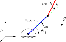
Figure 1: Schematic model of pendubot

Since much of the theory that is employed to synthesize the tracking control law rests on geometric ideas, our approach to the pendubot will proceed on such geometric lines, and exploit its Lie group structure. At first sight, this might seem an overkill for the two-link problem, but the logic of the control synthesis is more evident in the geometric setting. Further, the generalization to the $n$-link manipulator is more easily done employing the geometric framework.

The pendubot (in Figure 1) is a simple mechanical system which evolves on the manifold $SO(2)\times SO(2)$. To enable a matrix Lie group rooted approach to the problem, all the configuration variables in this article are expressed in $SO(2)$, since $S^{1}$ is diffeomorphic to $SO(2)$ by the map $f$ defined as:

$$f:S^{1}\to SO(2)\;\;\;\;f(e^{i\theta})\coloneq\begin{pmatrix}\sin\theta&-\cos\theta\\ \cos\theta&\sin\theta\end{pmatrix}$$

where, $e^{i\theta}=\cos\theta+i\sin\theta$ and $e^{i\theta}\in S^{1}$,
The kinetic energy of the two link robot is considered as the Riemannian metric. The moment of inertia about respective hinge points for link 1 (in blue) and link 2 (in red) are $\mathbb{I}_{1}$ and $\mathbb{I}_{2}$ respectively. $B_{1}$, $B_{2}$ are body fixed frames on link 1 and link 2 respectively and $I_{f}$ is the inertial frame. $R_{1},R_{2}\in SO(2)$ are rotation matrices from $B_{1}$ to $I_{f}$ and from $B_{2}$ to $B_{1}$ respectively. In Figure 1, $R_{i}=e^{i\theta_{i}}$. The center of mass of each rod is assumed to be at the midpoint. $\omega_{1}$ and $\omega_{2}$ are body velocities defined as $\hat{\omega}_{i}=R_{i}^{T}\dot{R}_{i}$ for $i=1,2$. Kinetic energy of the two link robot is given by

$$K(R_{1},R_{2},\omega_{1},\omega_{2})=\int_{B_{1}}||\dot{x}_{B_{1}}||^{2}\rho_{1}\mathrm{d}V_{1}+\int_{B_{1}}||\dot{x}_{B_{2}}||^{2}\rho_{2}\mathrm{d}V_{2}$$ (3)

where , $x_{B_{1}}=R_{1}X_{B_{1}}$, $x_{B_{2}}=R_{1}R_{2}X_{B_{2}}+R_{1}L_{1}$, $X_{B_{i}}$ is the position of a unit mass in the $i$th link in $I_{f}$ frame and, $L_{1}=\begin{pmatrix}0&l_{1}\end{pmatrix}^{T}$, $\rho_{i}$ is the density of $i$th link. Expanding (see Appendix -A for details) yields

$$K(\omega_{1},\omega_{2},R_{2})= \omega_{1}^{2}(\mathbb{I}_{1}+\mathbb{I}_{2}+m_{2}l_{1}^{2}+m_{2}L_{1}^{T}R_{2}L_{2})$$ (4)

$$+\omega_{1}\omega_{2}(2\mathbb{I}_{2}+m_{2}L_{1}^{T}R_{2}L_{2})+\mathbb{I}_{2}\omega_{2}^{2}$$

The potential energy is given by

$$V(R_{1},R_{2})=({{m_{1}\vbox to1.29167pt{}}\over{\vbox to1.29167pt{}2}}+m_{2})gl_{1}e_{1}^{T}R_{1}e_{1}+{{m_{2}\vbox to1.29167pt{}}\over{\vbox to1.29167pt{}2}}gl_{2}e_{1}^{T}R_{2}R_{1}e_{1}$$ (5)

where $e_{1}=\begin{pmatrix}1&0\end{pmatrix}^{T}$. The equations of motion are (see Appendix -B)

$$\dot{\omega}_{1}={{1\vbox to1.29167pt{}}\over{\vbox to1.29167pt{}2K_{1}}}(u_{1}-\Gamma_{1}-K_{2}\dot{\omega}_{2}-\alpha(2\omega_{1}+\omega_{2})) (2K_{3}-{{K_{2}^{2}\vbox to1.29167pt{}}\over{\vbox to1.29167pt{}2K_{1}}})\dot{\omega}_{2}= -{{K_{2}\vbox to1.29167pt{}}\over{\vbox to1.29167pt{}2K_{1}}}(u_{1}-\Gamma_{1}-\alpha(2\omega_{1}+\omega_{2})) -\alpha\omega_{1}+\beta(\omega_{1}^{2}+\omega_{1}\omega_{2})-\Gamma_{2}.$$ (6a) (6b)

where,

$$K_{1}=\mathbb{I}_{1}+\mathbb{I}_{2}+m_{2}l_{1}^{2}+m_{2}L_{1}^{T}R_{2}L_{2},$$

$$K_{2}=2\mathbb{I}_{2}+m_{2}L_{1}^{T}R_{2}L_{2},\quad K_{3}=\mathbb{I}_{2},$$

$$\alpha=m_{2}\langle L_{1}L_{2}^{T},R_{2}\hat{\omega}_{2}\rangle,\quad\beta=m_{2}{\{skew(R_{2}L_{1}L_{2}^{T})\}}\breve{},$$

$$\Gamma_{1}\coloneq(0.5{m_{1}}+m_{2})gl_{1}{\{skew(R_{1}e_{1}e_{1}^{T})\}}\breve{}$$

$$+0.5{m_{2}}gl_{2}{\{skew(R_{1}R_{2}^{T}e_{1}e_{1}^{T})\}}\breve{},$$

$$\Gamma_{2}\coloneq 0.5{m_{2}}gl_{2}{\{skew(R_{2}e_{1}e_{1}^{T}R_{1}^{T})\}}\breve{}.$$

IV Tracking control

In this section, we follow the procedure in Section V of [14] to define a tracking error and error dynamics for the unactuated joint. Let ${R_{2_{ref}}}:\mathbb{R}^{+}\to SO(2)$ be a smooth reference trajectory for joint 2 which has bounded velocity. The objective is to choose $u_{1}(t)$ in (6b) so that $R_{2}(t)$ tracks ${R_{2_{ref}}}(t)$ from almost all initial conditions with asymptotic convergence (this is almost-global tracking which we define later, in Definition 1). The almost-global tracking of $R_{2_{ref}}$ is achieved in two steps.

• In the first step, we define the error dynamics for the unactuated link which describes the evolution of the error trajectory. We ensure that the control input appears in this equation by substituting for the actuated variable in terms of the control.

• In the second step, in order to bring in an SMS structure to the unactuated dynamics, we define a new control which incorporates the additional terms resulting due to step 1. Once the system has the SMS structure, existing tracking laws are easily implemented. We then proceed to synthesize AGAT control.

We shall henceforth refer to this two-step procedure as the separation principle.

IV-A AGAS of error dynamics

Let us denote the angular velocity of the reference trajectory as ${\hat{\omega}}_{r}\coloneq{R_{2_{ref}}}^{T}\dot{R}_{2_{ref}}$. We then define a configuration error trajectory$E(t)\coloneq{R_{2_{ref}}}(t)R_{2}^{T}(t)$ on $SO(2)$. The velocity of this error trajectory is given as

$$\dot{E}={R_{2_{ref}}}({\hat{\omega}}_{r}-{\hat{\omega}}_{2})R_{2}^{T}$$ (7)

Next, we define a closed loop energy like function $E_{cl}:TSO(2)\to\mathbb{R}$ as follows

$$E_{cl}(E,\dot{E})=K_{p}\psi(E)+{{1\vbox to1.29167pt{}}\over{\vbox to1.29167pt{}2}}{||\dot{E}||_{\mathbb{G}_{\mathbb{I}}}}^{2}$$ (8)

where $\mathbb{G}_{\mathbb{I}}$ is the metric induced on $SO(2)$ by the $\mathbb{I}$ (see section 5.3.1 in [4] for more details), $\mathbb{I}\coloneq 2K_{3}-{{K_{2}^{2}\vbox to1.29167pt{}}\over{\vbox to0.90417pt{}2K_{1}}}$, $\psi(E)\coloneq tr\{P(id-E)\}$, $id$ denotes the $2\times 2$ identity matrix, $P\coloneq diag(c_{1},c_{2})$, and $c_{1}+c_{2}\neq 0$.

Remark 1.

At this stage the problem is entirely focused on $SO(2)$.

Definition 1.

The reference trajectory $R_{2_{ref}}$ is almost-globally stable with respect to the closed loop energy like function $E_{cl}$ (defined in (8)) if, for almost all initial conditions $(R_{2}(0),\omega_{2}(0))\in SO(2)\times\mathfrak{so(2)}$, the function $t\to E_{cl}(t)$ is non-increasing.

Definition 2.

The Hessian of $\psi$ is the symmetric $(0,2)$ tensor field denoted by $Hess\psi$ and defined as $Hess\psi(q)(v_{q},w_{q})=\mathbb{G}_{\mathbb{I}}(v_{q},\stackrel{{\scriptstyle\mathbb{G}_{\mathbb{I}}}}{{\nabla}}_{w_{q}}grad\psi),$ where $v_{q}$, $w_{q}\in T_{q}SO(2)$ and $grad$ denotes the gradient vector field.

If $x_{0}$ is a critical point of $\psi$ and $\theta$ is the local coordinate at $x_{0}$, then, $Hess(\psi)(x_{0})$ in coordinates is $Hess\psi(x_{0})={{\partial^{2}\psi\vbox to1.29167pt{}}\over{\vbox to0.90417pt{}\partial\theta^{2}}}(x_{0})$ (see chapter 13 in [13] for details)

Definition 3.

([8]) A function $\psi:SO(2)\to\mathbb{R}$ on $(SO(2),\mathbb{G}_{\mathbb{I}})$ is a navigation function if

1. $\psi$ attains a unique minimum.

2. $Det(Hess\psi(q^{*}))\neq 0$ whenever $\mathrm{d}\psi(q^{*})=0$ for some $q^{*}\in SO(2)$.

Lemma 1.

$\psi$ is a navigation function on $SO(2)$.

Proof.

We proceed to determine the critical points of $\psi:SO(2)\to\mathbb{R}$.

$${{\mathrm{d}\vbox to1.29167pt{}}\over{\vbox to1.29167pt{}\mathrm{d}t}}\psi(E) =-tr(P\dot{E})=-tr(PEE^{T}\dot{E})$$

$$=-tr\big{(}(skew(PE)+sym(PE))(E^{T}\dot{E})\big{)}$$

$$=2{\{skew(PE)\}}\breve{}\quad\{E^{T}\dot{E}\}\breve{}$$

The third step follows from the equality $tr(xy)=-\hat{x}\hat{y}$ and the fact that $E^{T}\dot{E}\in\mathfrak{so(2)}$ is skew symmetric. Therefore, the critical points of $\psi$ are the solution to the equation $skew(PE)=0_{2\times 2}$ or, $PE=E^{T}P$. Let $E=\begin{pmatrix}x&y\\ -y&x\end{pmatrix}$ where $x^{2}+y^{2}=1$, therefore, $skew(PE)=\begin{pmatrix}0&y(c_{1}+c_{2})\\ -y(c_{1}+c_{2})&0\end{pmatrix}$. So, the two critical configurations are given by $\begin{pmatrix}1&0\\ 0&1\end{pmatrix}$ and $\begin{pmatrix}-1&0\\ 0&-1\end{pmatrix}$. Observe that $\psi(E)=tr(P(id-E))=(1-x)(c_{1}+c_{2})$ and hence, that $id$ is the unique minimum and $-id$ is the unique maximum of $\psi$. It is verified that the Hessian is positive definite at both critical points along the lines of Proposition 11.31 in [4]. ∎

We choose the error dynamics for AGAT of $R_{2_{ref}}$ as the SMS $(SO(2),\mathbb{G}_{\mathbb{I}},-K_{p}\mathrm{d}\psi(E)+F_{d}\dot{E})$, where, $F_{d}$ is a dissipative force, and, $K_{p}$ and $\psi$ are defined in (8). Then the error dynamics are given by the following equations

$$\stackrel{{\scriptstyle\mathbb{G}_{\mathbb{I}}}}{{\nabla}}_{\dot{E}}\dot{E}=\mathbb{G}^{\sharp}_{\mathbb{I}}(-K_{p}\mathrm{d}\psi(E)+F_{d}\dot{E})$$ (9)

Lemma 2.

The error dynamics in (9) is almost-globally asymptotically stable about $(E^{*},\dot{E}^{*})=(id,0)$

Proof.

Observe that $E_{cl}(id,0)=0$ and $E_{cl}(q,0)>0$ for all $(q,0)\in TSO(2)$ in a neighborhood of $(id,0)$. Also,

$${{\mathrm{d}\vbox to1.29167pt{}}\over{\vbox to1.29167pt{}\mathrm{d}t}}E_{cl}(E,\dot{E}) =\langle K_{p}\mathrm{d}\psi(E),\dot{E}\rangle+\ll\dot{E},\stackrel{{\scriptstyle\mathbb{G}_{\mathbb{I}}}}{{\nabla}}_{\dot{E}}\dot{E}\gg$$

$$=\langle K_{p}\mathrm{d}\psi(E),\dot{E}\rangle$$

$$+\mathbb{G}_{\mathbb{I}}(\dot{E},-\mathbb{G}_{\mathbb{I}}^{\sharp}(K_{p}\mathrm{d}\psi(E)-F_{d}(\dot{E}))$$

$$=K_{p}\langle\mathrm{d}\psi,\dot{E}\rangle-K_{p}\langle\mathrm{d}\psi,\dot{E}\rangle+\langle F_{d}(\dot{E}),\dot{E}\rangle\leq 0$$

as $F_{d}$ is dissipative. Therefore $E_{cl}$ is a Lyapunov function and the error dynamics in (9) is locally stable around $(id,0)$. The almost-global stability result follows from Lemma 1 in [14] as $\psi$ is a navigation function, $E(g,g)=id$ for all $g\in SO(2)$ and $(\psi,E)$ is a compatible pair. ∎

Remark 2.

The ’zero error’ equilibrium state mentioned in the beginning of this section is $(id,0)$. The configuration at which the navigation function achieves its minimum is the ’zero error’ configuration and the RHS of (9) is the control vector field which drives the error trajectory to $(id,0)$.

IV-B Separation principle and AGAT of $R_{2_{ref}}(t)$

The separation principle has two important steps. For the first step, the LHS of (9) is expressed in terms of the trajectories $R_{2}(t)$, $R_{2_{ref}}(t)$ and their velocities. For the second step the feedback terms to be introduced through $u_{1}$ are identified. The following theorem states the main result of this paper.

Theorem 1.

Consider the pendubot described by equations (6a)-(6b), the smooth bounded reference trajectory ${R_{2_{ref}}}:\mathbb{R}^{+}\to SO(2)$ is almost-globally asymptotically tracked by the control law

$$u_{1}= {{2K_{1}\vbox to1.29167pt{}}\over{\vbox to1.29167pt{}K_{2}}}\bigg{\{}\underbrace{\{Ad_{R_{2}}^{*}u\}\breve{}}_{\text{PD term}}$$ (10)

$$+\underbrace{{{K_{2}\vbox to1.29167pt{}}\over{\vbox to1.29167pt{}2K_{1}}}(\alpha(2\omega_{1}+\omega_{2})+\Gamma_{1})-\alpha\omega_{1}+\beta(\omega_{1}^{2}+\omega_{1}\omega_{2})-\Gamma_{2}}_{\text{cancelling the quadratic terms}}$$

$$-\underbrace{\{\mathbb{I}(\dot{{\hat{\omega}}}_{r}+[{\hat{\omega}}_{2},{\hat{\omega}}_{r}])\}\breve{}\quad}_{\text{feedforward terms}}\bigg{\}}$$

where $R_{2}(t)$ is the controlled trajectory for link 2, and $u\in\mathfrak{g}^{*}$ is defined as $u=E^{T}(-2K_{p}skew(PE)+F_{d}\dot{E})$.

Proof.

Let the body velocity of the error trajectory be defined as $\eta\coloneq T_{E}L_{E^{-1}}\dot{E}$. The LHS of (9) can be simplified as follows

$$\stackrel{{\scriptstyle\mathbb{G}_{\mathbb{I}}}}{{\nabla}}_{\dot{E}}\dot{E} =T_{id}L_{E}\{{{\mathrm{d}\vbox to1.29167pt{}}\over{\vbox to1.29167pt{}\mathrm{d}t}}(E^{T}\dot{E})+\stackrel{{\scriptstyle\mathfrak{so(2)}}}{{\nabla}}_{\eta}\eta\}$$ (11)

$$=T_{id}L_{E}\{-R_{2}\dot{\hat{\omega}}_{2}R_{2}^{T}+R_{2}([\hat{\omega}_{2},\hat{\omega}_{r}]-\dot{\hat{\omega}}_{2})R_{2}^{T}+\stackrel{{\scriptstyle\mathfrak{so(2)}}}{{\nabla}}_{\eta}\eta\}$$

$$=T_{id}L_{E}\{-R_{2}\dot{\omega}_{2}R_{2}^{T}+R_{2}([\hat{\omega}_{2},\hat{\omega}_{r}]+\dot{\hat{\omega}}_{r})R_{2}^{T}\}$$

The first equality follows from Lemma 3 in [15]. The second equality is given by the following simplification

$${{\mathrm{d}\vbox to1.29167pt{}}\over{\vbox to1.29167pt{}\mathrm{d}t}}(E^{T}\dot{E}) ={{\mathrm{d}\vbox to1.29167pt{}}\over{\vbox to1.29167pt{}\mathrm{d}t}}\{E^{T}R_{2_{ref}}({\hat{\omega}}_{r}-{\hat{\omega}}_{2})R_{2}^{T}\}$$

$$={{\mathrm{d}\vbox to1.29167pt{}}\over{\vbox to1.29167pt{}\mathrm{d}t}}\{R_{2}({\hat{\omega}}_{r}-{\hat{\omega}}_{2})R_{2}^{T}\}$$

$$=\dot{R}_{2}\hat{\omega}_{r}R_{2}^{T}+R_{2}\dot{\hat{\omega}}_{r}R_{2}^{T}-R_{2}\hat{\omega}_{r}R_{2}^{T}\dot{R}_{2}R_{2}^{T}$$

$$-\dot{R}_{2}\hat{\omega}_{2}R_{2}^{T}-R_{2}\dot{\hat{\omega}}_{2}R_{2}^{T}+R_{2}\hat{\omega}_{2}R_{2}^{T}\dot{R}_{2}R_{2}^{T}$$

$$=R_{2}(\dot{\hat{\omega}}_{r}+[\hat{\omega}_{2},\hat{\omega}_{r}]-\dot{\hat{\omega}}_{2})R_{2}^{T}$$

The third equality follows from the fact that $SO(2)$ is Abelian, and therefore, $\stackrel{{\scriptstyle\mathfrak{g}}}{{\nabla}}_{\eta}\eta=0$.
Observe (from (9)) that $\stackrel{{\scriptstyle\mathbb{G}_{\mathbb{I}}}}{{\nabla}}_{\dot{E}}\dot{E}=T_{id}L_{E}\mathbb{I}^{\sharp}(u)$, where $u=E^{T}(-2K_{p}skew(PE)+F_{d}\dot{E})$ is the stabilizing control. Now from (11),

$$\mathbb{I}^{\sharp}(u)=-R_{2}\dot{\omega}_{2}R_{2}^{T}+R_{2}([\hat{\omega}_{2},\hat{\omega}_{r}]+\dot{\hat{\omega}}_{r})R_{2}^{T}$$

Rearranging the above equation leads to

$$\mathbb{I}\dot{\omega}_{2} =-Ad_{R_{2}}^{*}(u-\mathbb{I}Ad_{R_{2}}([\hat{\omega}_{2},\hat{\omega}_{r}]-\dot{\hat{\omega}}_{2}))$$ (12)

$$=-Ad_{R_{2}}^{*}u+\mathbb{I}(\dot{{\hat{\omega}}}_{r}+[{\hat{\omega}}_{2},{\hat{\omega}}_{r}])$$

However, from (6b) we have,

$$\mathbb{I}\dot{\omega}_{2}= -{{K_{2}\vbox to1.29167pt{}}\over{\vbox to1.29167pt{}2K_{1}}}(u_{1})+{{K_{2}\vbox to1.29167pt{}}\over{\vbox to1.29167pt{}2K_{1}}}(\alpha(2\omega_{1}+\omega_{2})+\Gamma_{1})-\alpha\omega_{1}$$ (13)

$$+\beta(\omega_{1}^{2}+\omega_{1}\omega_{2})-\Gamma_{2}$$

Comparing (12) and (13) yields the expression for $u_{1}$ as in (10). Essentially, we cancel out the last three terms of (13) and introduce the proportional derivative (or PD) control in (12) through $-{{K_{2}\vbox to1.29167pt{}}\over{\vbox to0.90417pt{}2K_{1}}}(u_{1})$. By Lemma 2, the error dynamics for the tracking problem (in (9)) is almost-globally asymptotically stable about $(id,0)$. Therefore, $u_{1}$ is the desired control for almost-global tracking of ${R_{2_{ref}}}(t)$. ∎

Remark 3.

In the control law (10), the terms $\{Ad_{R_{2}}^{*}u\}\breve{}-\{\mathbb{I}(\dot{{\hat{\omega}}}_{r}+[{\hat{\omega}}_{2},{\hat{\omega}}_{r}])\}\breve{}$ denote the PD plus feed-forward terms for AGAS of the error dynamics. The remaining terms are the quadratic terms that essentially cancel out identical terms in (13) and impart the SMS structure to the error dynamics (in (12)).

Remark 4.

Note that the cancellation of the quadratic terms is not to be mistaken to be feedback linearization; it is an operation solely from a mechanics point of view to impart a mechanical structure to the error dynamics. This feature is elaborated in [9].

V AGAT of unactuated links of an $n$-link robot

Consider an $n$-link robot with $m$ actuated (or active) links and $l$ unactuated (or passive) links. Let $q_{1}\in\underbrace{SO(2)\times\dotsc\times SO(2)}_{\text{m times}}$ and $q_{2}\in\underbrace{SO(2)\times\dotsc\times SO(2)}_{\text{l times}}$ denote the generalized variables of active and passive links respectively. The equations of motion can be expressed as

$$M_{11}\ddot{q}_{1}+M_{12}\ddot{q}_{2}+h_{1}+\Phi_{1}=u_{1} M_{21}\ddot{q}_{1}+M_{22}\ddot{q}_{2}+h_{2}+\Phi_{2}=0$$ (14a) (14b)

where $M_{11}\in\mathbb{R}^{m\times m}$, $M_{12}\in\mathbb{R}^{m\times l}$, $M_{21}\in\mathbb{R}^{l\times m}$ and $M_{22}\in\mathbb{R}^{l\times l}$. $h_{1}$ and $h_{2}$ contain Coriolis and centrifugal terms (quadratic velocity terms), $\Phi_{1}$, $\Phi_{2}$ contain gravitational terms and, $u_{1}\in T_{q_{1}}\underbrace{SO(2)\times\dotsc\times SO(2)}_{\text{m times}}$ is the control vector field to be chosen such that $q_{2}(t)$ tracks a given reference trajectory $q_{2_{ref}}(t)$. The equations (14a)-(14b) can be simplified as follows

$$\ddot{q}_{1}=M_{11}^{-1}(u_{1}-\Phi_{1}-h_{1}-M_{12}\ddot{q}_{2})$$ (15a)

$$(M_{22}-M_{21}M_{11}^{-1}M_{12})\ddot{q}_{2} -M_{21}M_{11}^{-1}(h_{1}+\Phi_{1})+h_{2}+\Phi_{2}$$ (15b)

$$=-M_{21}M_{11}^{-1}u_{1}$$

Remark 5.

$\mathbb{I}\coloneq M_{22}-M_{21}M_{11}^{-1}M_{12}$ is invertible as it is the Schur complement of the invertible mass matrix $M\coloneq\begin{pmatrix}M_{11}&M_{12}\\ M_{21}&M_{22}\end{pmatrix}$.

Let $q_{2_{ref}}(t)\in G$ denote the reference trajectory, where $G=\underbrace{SO(2)\times\dotsc\times SO(2)}_{\text{l times}}$. The group operation is defined component-wise as $L_{(g_{1},\dotsc,g_{l})}(h_{1},\dotsc,h_{l})=(g_{1}h_{1},\dotsc,g_{l}h_{l})$. Similar to Section IV, we first express the error dynamics for the tracking problem. Let $E=q_{2_{ref}}(t)q_{2}^{-1}(t)$ be the error trajectory. The error is identity when the $q_{2}(t)$ coincides with $q_{2_{ref}}(t)$. The error dynamics is given by (9). Simplifying the LHS of (9), we have,

$$\stackrel{{\scriptstyle\mathbb{G}_{\mathbb{I}}}}{{\nabla}}_{\dot{E}}\dot{E} =T_{id}L_{E}\{{{\mathrm{d}\vbox to1.29167pt{}}\over{\vbox to1.29167pt{}\mathrm{d}t}}(E^{T}\dot{E})+\stackrel{{\scriptstyle\mathfrak{g}}}{{\nabla}}_{\eta}\eta\}$$ (16)

$$=T_{id}L_{E}\{\ddot{q}_{2}q_{2}^{-1}+{\stackrel{{\scriptstyle\mathfrak{g}}}{{\nabla}}}_{\eta}\eta+{{\mathrm{d}\vbox to1.29167pt{}}\over{\vbox to1.29167pt{}\mathrm{d}t}}(\dot{q}_{2_{ref}}q_{2_{ref}}^{-1})\}$$

where $\eta\coloneq E^{-1}\dot{E}$. In the following theorem we state the necessary condition for AGAT of $q_{2_{ref}}(t)$.

Theorem 2.

Consider the $n$-link pendubot described by the equations (14a)-(14b) and the smooth bounded reference trajectory $q_{2_{ref}}:\mathbb{R}\to G$. If $rank(M_{21})\geq l$ ($M_{21}$ has full column rank), then the following $u_{1}$ is the control vector field so that $q_{2}(t)$ almost-globally and asymptotically tracks $q_{2_{ref}}(t)$.

$$u_{1} =M_{11}M_{21}^{-1}(T_{e}R_{q_{2}}(u-\mathbb{I}\{{\stackrel{{\scriptstyle\mathfrak{g}}}{{\nabla}}}_{\eta}\eta+{{\mathrm{d}\vbox to1.29167pt{}}\over{\vbox to1.29167pt{}\mathrm{d}t}}(\dot{q}_{2_{ref}}q_{2_{ref}}^{-1})\})$$ (17)

$$+h_{2}-M_{21}M_{11}^{-1}h_{1})$$

where $u=E^{T}(-K_{p}\mathrm{d}\phi(E)+F_{d}\dot{E})$ and $\phi$ is a navigation function on $G$.

Proof.

From (9), we have $\stackrel{{\scriptstyle\mathbb{G}_{\mathbb{I}}}}{{\nabla}}_{\dot{E}}\dot{E}=T_{id}L_{E}\mathbb{I}^{\sharp}u$, where $u=E^{T}(-K_{p}\mathrm{d}\psi(E)+F_{d}\dot{E})$ and $\phi$ is a navigation function on $G$. Substituting $T_{id}L_{E}\mathbb{I}^{\sharp}u$ in the LHS of (16), we obtain

$$u=\mathbb{I}\ddot{q}_{2}q_{2}^{-1}+\mathbb{I}\{{\stackrel{{\scriptstyle\mathfrak{g}}}{{\nabla}}}_{\eta}\eta+{{\mathrm{d}\vbox to1.29167pt{}}\over{\vbox to1.29167pt{}\mathrm{d}t}}(\dot{q}_{2_{ref}}q_{2_{ref}}^{-1})\}$$ (18)

Substituting for $\mathbb{I}\ddot{q}_{2}$ from (15b), we have,

$$u =(M_{21}M_{11}^{-1}h_{1}-h_{2}+M_{21}M_{11}^{-1}u_{1})q_{2}^{-1}$$ (19)

$$+\mathbb{I}\{{\stackrel{{\scriptstyle\mathfrak{g}}}{{\nabla}}}_{\eta}\eta+{{\mathrm{d}\vbox to1.29167pt{}}\over{\vbox to1.29167pt{}\mathrm{d}t}}(\dot{q}_{2_{ref}}q_{2_{ref}}^{-1})\}$$

This implies,

$$M_{21}M_{11}^{-1}u_{1} =T_{e}R_{q_{2}}(u-\mathbb{I}\{{\stackrel{{\scriptstyle\mathfrak{g}}}{{\nabla}}}_{\eta}\eta+{{\mathrm{d}\vbox to1.29167pt{}}\over{\vbox to1.29167pt{}\mathrm{d}t}}(\dot{q}_{2_{ref}}q_{2_{ref}}^{-1})\})$$ (20)

$$+h_{2}+\Phi_{2}-M_{21}M_{11}^{-1}(h_{1}+\Phi_{1}).$$

As, $M_{21}$ has full column rank, therefore, $M_{21}^{-1}$ exists, hence,

$$u_{1}= M_{11}M_{21}^{-1}(T_{e}R_{q_{2}}(u-\mathbb{I}\{{\stackrel{{\scriptstyle\mathfrak{g}}}{{\nabla}}}_{\eta}\eta+{{\mathrm{d}\vbox to1.29167pt{}}\over{\vbox to1.29167pt{}\mathrm{d}t}}(\dot{q}_{2_{ref}}q_{2_{ref}}^{-1})\})$$ (21)

$$+h_{2}+\Phi_{2}-M_{21}M_{11}^{-1}(h_{1}+\Phi_{1})).$$

Therefore, using a separation principle, we have introduced terms through $u_{1}$, so that the error dynamics in (9) retains its SMS structure. As $\phi$ is a navigation function, by a proof similar to Lemma 2, the error dynamics is AGAS about $(e,0)$ where $e$ is the identity of $G$. Therefore, $u_{1}$ is the desired control for AGAT of $q_{2_{ref}}(t)$. ∎

Remark 6.

The condition imposed on $M_{21}$ is called ’strong inertial coupling’ which means that the number of active degrees of freedom must be atleast as many as the passive degrees in order to solve the tracking problem. This is also observed by the authors in [21]. However, in [21], the authors use a partial feedback linearization approach to achieve local tracking, which means the initial conditions of the system are close to the initial conditions of the reference trajectory. In both Theorems 1 and 2, the initial conditions of the unactuated joint(s) of the pendubot are allowed to lie in a dense set in $T(SO(2))$ and $TG$ respectively.

Remark 7.

The navigation function $\phi$ in Theorem 2 which is necessary for AGAS of the error dynamics can be obtained by composing $\psi$ (in $SO(2)$) $l$ times, as elaborated in Section 3 in [5].

VI Simulation results

For the purpose of simulation, the parameters of the pendubot are: $m_{1}=0.25kg$, $m_{2}=0.2kg$, $l_{1}=l_{2}=0.5m$, $g=9.8ms^{-2}$ with the following initial conditions:

$$R_{1}(0)=\begin{pmatrix}1&0\\ 0&1\end{pmatrix},\;\;\omega_{1}(0)=-1\quad rads^{-1},$$

$$R_{2}(0)=\begin{pmatrix}0.4794&0.87758\\ -0.87758&0.4794\end{pmatrix},\;\;\omega_{2}(0)=2\quad rads^{-1}$$

The reference trajectory is given by

$$R_{2_{ref}}(t)=\begin{pmatrix}\sin(t+\pi/4)&\cos(t+\pi/4)\\ -\cos(t+\pi/4)&\sin(t+\pi/4)\end{pmatrix},\;$$

$$\omega_{2_{ref}}(t)=1\quad rads^{-1},\;t\geq 0.$$

The AGAT control in (10) is implemented by considering $K_{p}=2.3$, $F_{d}=-diag(1.5\quad 2)$, $P=diag(1\quad 1.5)$. In this simulation and all others to follow, the differential equations are solved using MATLAB 2014a and the trajectory for the second link (in blue) is compared with the reference trajectory (in red). The first two subfigures plot $R_{2}(11)=cos(\theta_{1})$ with $R_{2_{ref}}(11)$ and $R_{2}(12)=sin(\theta_{1})$ with $R_{2_{ref}}(12)$ respectively. Therefore, they correspond to $x$ and $y$ coordinates in a circle embedded in $\mathbb{R}^{2}$. The third subfigure shows the first coordinate $E(11)$ of $E(t)\in SO(2)$. As, $E(t)\to id$, it is seen that $E(11)$ converges to $1$. The fourth subfigure shows control effort $|u_{1}|$. In the fifth subfigure, we plot $\omega_{1}(t)$ and observe that it remains bounded. The first simulation results are shown in Figure  2.

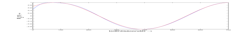
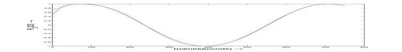
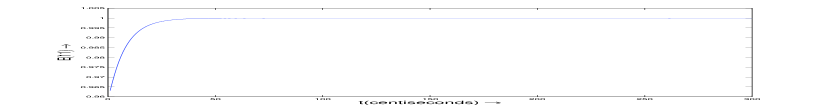
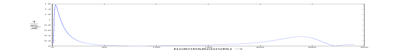
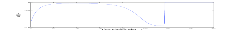
Figure 2: Tracking results for the first two coordinates for the initial condition $R_{2}(0)=\begin{pmatrix}0.4794&0.87758\\ -0.87758&0.4794\end{pmatrix}$ in

For the second simulation we choose the following initial conditions:

$$R_{1}(0)=\begin{pmatrix}1&0\\ 0&1\end{pmatrix},\;\;\;\omega_{1}(0)=-1\quad rads^{-1}$$

$$R_{2}(0)=\begin{pmatrix}0&1\\ -1&0\end{pmatrix},\;\;\;\omega_{2}(0)=2\quad rads^{-1}$$

The reference trajectory is chosen to be:

$$R_{2_{ref}}(t)=\begin{pmatrix}\cos(t)&-\sin(t)\\ \sin(t)&\cos(t)\end{pmatrix},\;\;\omega_{2_{ref}}(t)=1\quad rads^{-1},\;\;t\geq 0.$$

We consider $K_{p}=3$, $F_{d}=-diag(1.5\quad 2)$, $P=diag(2\quad 1.5)$. Figure 3 shows the results. The last subfigure depicts the reference and the actual trajectory on a cylinder

Now for the same initial conditions for the pendubot, we consider

$$R_{2_{ref}}(t)=id,\;\;\omega_{2_{ref}}(0)=0\quad rads^{-1},\;\forall t\geq 0$$

This is therefore, a stabilization problem. The results are shown in Figure 4.

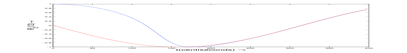
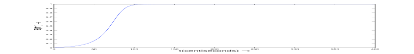
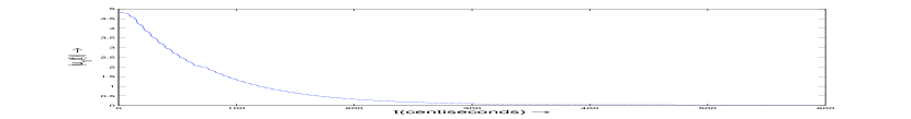
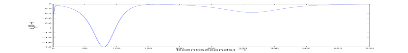
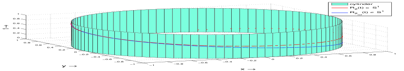
Figure 3: Tracking results for second set of initial conditions and, $R_{2_{ref}}(t)=\begin{pmatrix}\cos(t)&-\sin(t)\\ \sin(t)&\cos(t)\end{pmatrix}.$

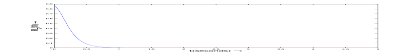
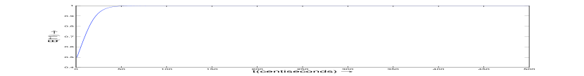
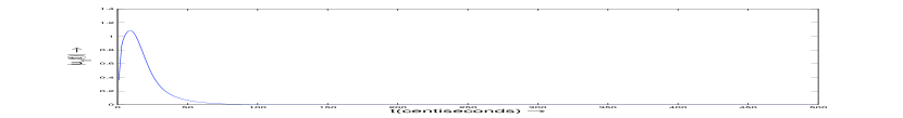
Figure 4: Tracking results for second set of initial conditions and, $R_{2_{ref}}(t)=id$

$$R_{1}(0)=\begin{pmatrix}1&0\\ 0&1\end{pmatrix},\;\;\omega_{1}(0)=-1\quad rads^{-1}$$

$$R_{2}(0)=\begin{pmatrix}0.4794&0.87758\\ -0.87758&0.4794\end{pmatrix},\;\;\omega_{2}(0)=2\quad rads^{-1}$$

The reference trajectory is chosen to be:

$$R_{2_{ref}}(t)=\begin{pmatrix}-\cos(t)&\sin(t)\\ -\sin(t)&-\cos(t)\end{pmatrix},\;\;\omega_{2_{ref}}(t)=1\quad rads^{-1},\;t\geq 0.$$

We consider $K_{p}=2.5$, $F_{d}=-diag(1.5\quad 2.2)$, $P=diag(2\quad 1.5)$. The results are shown in Figure  5.

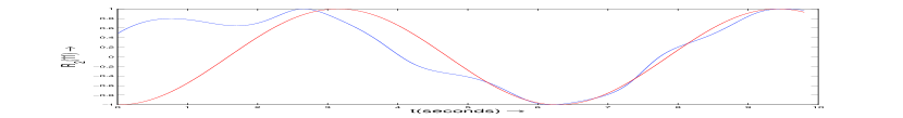
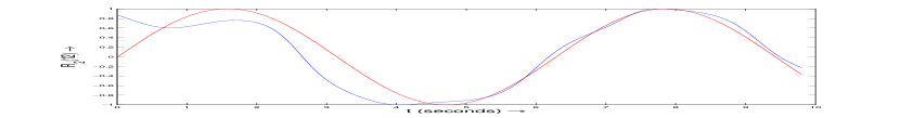
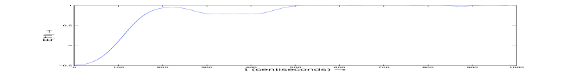
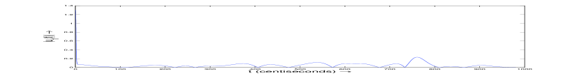
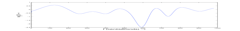
Figure 5: Tracking results for the last set of initial conditions

Next, we consider another pendubot with the following parameters: $m_{1}=0.1kg$, $m_{2}=0.4kg$, $l_{1}=0.25\quad m$ and $l_{2}=0.5\quad m$. The second set of initial conditions is considered along with:

$$R_{2_{ref}}(t)=\begin{pmatrix}\cos(t)&-\sin(t)\\ \sin(t)&\cos(t)\end{pmatrix},\;\;\omega_{2_{ref}}(t)=1\quad rads^{-1},\;t\geq 0.$$

Simulations are performed with $K_{p}=5$, $F_{d}=-diag(1.5\quad 2.5)$, $P=diag(1.5\quad 1.3)$ and results are plotted in Figure 6.

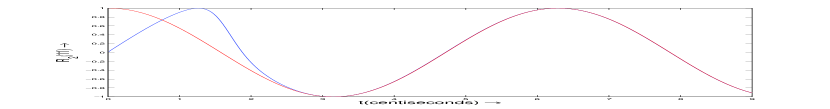
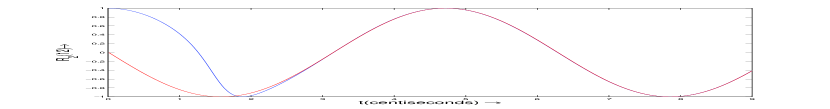
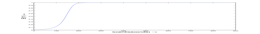
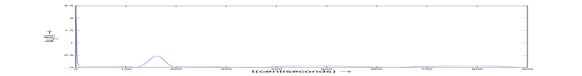
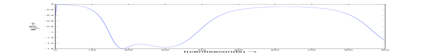
Figure 6: Tracking results for the second pendubot

VII Conclusions

By transforming the dynamical equation governing the unactuated coordinate into an SMS through a suitable transformation of the input, and then adopting standard techniques for tracking control, we synthesize a tracking control law for the unactuated variable. A few features of the control law, the simulations for an $n$-link manipulator and drawing conclusions based on the performance, constitute some ongoing work.

-A Kinetic energy

In what follows, we derive the expression for kinetic energy of the pendubot in (4).

$$\dot{x}_{B_{1}} =\dot{R}_{1}X_{B_{1}}$$ (22)

$$\dot{x}_{B_{2}} =\dot{R}_{1}L_{1}+(\dot{R}_{1}R_{2}+{R}_{1}\dot{R}_{2})X_{B_{2}}$$

Therefore,

$$||\dot{x}_{B_{1}}||^{2} =\langle\dot{R}_{1}X_{B_{1}},\dot{R}_{1}X_{B_{1}}\rangle=\langle\hat{\omega}_{1}X_{B_{1}},\hat{\omega}_{1}X_{B_{1}}\rangle$$ (23)

$$=(\hat{\omega}_{1}X_{B_{1}})^{T}(\hat{\omega}_{1}X_{B_{1}})=\Omega^{T}(\hat{\omega}_{1}X_{B_{1}}\times X_{B_{1}}).$$

where $\Omega=\begin{pmatrix}0&0&\omega\end{pmatrix}^{T}$. From (23), the first term in (3) is

$$\int_{B_{1}}||\dot{x}_{B_{1}}||^{2}\rho_{1}\mathrm{d}V_{1}=\int_{B_{1}}\Omega^{T}(\hat{\omega}_{1}X_{B_{1}}\times X_{B_{1}})\rho_{1}\mathrm{d}V_{1}=\mathbb{I}_{1}\omega^{2}_{1}.$$ (24)

From (22),

$$||\dot{x}_{B_{2}}||^{2} =\langle\dot{R}_{1}L_{1},\dot{R}_{1}L_{1}\rangle+2\langle\dot{R}_{1}L_{1},(\dot{R}_{1}R_{2}+{R}_{1}\dot{R}_{2})X_{B_{2}}\rangle$$ (25)

$$+\langle(\dot{R}_{1}R_{2}+{R}_{1}\dot{R}_{2})X_{B_{2}},(\dot{R}_{1}R_{2}+{R}_{1}\dot{R}_{2})X_{B_{2}}\rangle$$

$$=\langle\hat{\omega}_{1}L_{1},\hat{\omega}_{1}L_{1}\rangle+2\langle\hat{\omega}_{1}L_{1},(\hat{\omega}_{1}R_{2}+R_{2}\hat{\omega}_{2})X_{B_{2}}\rangle$$

$$+\langle(\hat{\omega}_{1}R_{2}+R_{2}\hat{\omega}_{2})X_{B_{2}},(\hat{\omega}_{1}R_{2}+R_{2}\hat{\omega}_{2})X_{B_{2}}\rangle$$

$$=\langle\hat{\omega}_{1}L_{1},\hat{\omega}_{1}L_{1}\rangle+2(\langle\hat{\omega}_{1}L_{1},\hat{\omega}_{1}(R_{2}X_{B_{2}})\rangle$$

$$+\langle\hat{\omega}_{1}L_{1},R_{2}\hat{\omega}_{2}L_{2}\rangle)$$

$$+\langle(\hat{\omega}_{1}R_{2}+R_{2}\hat{\omega}_{2})X_{B_{2}},(\hat{\omega}_{1}R_{2}+R_{2}\hat{\omega}_{2})X_{B_{2}}\rangle$$

We expand the second term in (25),

$$T_{2}\coloneq 2\langle\hat{\omega}_{1}L_{1},\hat{\omega}_{1}(R_{2}X_{B_{2}})\rangle+2\langle\hat{\omega}_{1}L_{1},R_{2}\hat{\omega}_{2}L_{2}\rangle$$

$$=2\langle\Omega_{1},(R_{2}X_{B_{2}})\times(\hat{\omega}_{1}L_{1})\rangle$$

$$+2\langle\Omega_{1},L_{1}\times R_{2}(\hat{\omega}_{2}X_{B_{2}})\rangle$$

$$=2\langle\Omega_{1},(L_{1}^{T}R_{2}X_{B_{2}})\Omega_{1}-((R_{2}X_{B_{2}})^{T}\Omega_{1})L_{1}\rangle$$

$$+2\langle\Omega_{1},(L_{1}^{T}R_{2}X_{B_{2}})(R_{2}\Omega_{2})-(L_{1}^{T}R_{2}\Omega_{2})R_{2}X_{B_{2}}\rangle$$

$$=2\langle\Omega_{1},(L_{1}^{T}R_{2}X_{B_{2}})(\Omega_{1}+\Omega_{2})\rangle$$

as $(R_{2}X_{B_{2}})^{T}\Omega_{1}=0$, $R_{2}\Omega_{2}=\Omega_{2}$ and, $L_{1}^{T}\Omega_{2}=0$.
The third term in (25) is

$$T_{3}\coloneq\langle(\hat{\omega}_{1}R_{2}+R_{2}\hat{\omega}_{2})X_{B_{2}},(\hat{\omega}_{1}R_{2}+R_{2}\hat{\omega}_{2})X_{B_{2}}\rangle$$

$$=\langle\hat{\omega}_{1}R_{2}X_{B_{2}},\hat{\omega}_{1}R_{2}X_{B_{2}}\rangle+2\langle R_{2}\hat{\omega}_{2}X_{B_{2}},\hat{\omega}_{1}R_{2}X_{B_{2}}\rangle$$

$$+\langle R_{2}\hat{\omega}_{2}X_{B_{2}},R_{2}\hat{\omega}_{2}X_{B_{2}}\rangle$$

$$=\langle\hat{\omega}_{1}(R_{2}X_{B_{2}}\times\hat{\omega}_{1}R_{2}X_{B_{2}})\rangle+\langle\hat{\omega}_{1},R_{2}(X_{B_{2}}\times\hat{\omega_{2}}X_{B_{2}})$$

$$+\langle\hat{\omega}_{2}X_{B_{2}},\hat{\omega}_{2}X_{B_{2}}\rangle$$

Observe that,

$$\int_{B_{2}}T_{2}\rho_{2}\mathrm{d}V_{2}=m_{2}(L_{1}^{T}R_{2}L_{2})(\omega_{1}^{2}+\omega_{1}\omega_{2})$$

as $\int_{B_{2}}X_{B_{2}}\rho_{2}\mathrm{d}V_{2}=L_{2}/2$ and,

$$\int_{B_{2}}T_{3}\rho_{2}\mathrm{d}V_{2}=\mathbb{I}_{2}\omega_{1}^{2}+2\mathbb{I}_{2}\omega_{1}\omega_{2}+\mathbb{I}_{2}\omega_{2}^{2}$$

as $\mathbb{I}_{2}(v)=\int_{B_{2}}X_{B_{2}}\times(\hat{v}X_{B_{2}})\rho_{2}\mathrm{d}V_{2}$ for $v\in\mathbb{R}^{3}$. From (25), the second term in (3) is

$$\int_{B_{2}}||\dot{x}_{B_{2}}||^{2}\rho_{2}\mathrm{d}V_{2} =\int_{B_{2}}\langle\hat{\omega}_{1}L_{1},\hat{\omega}_{1}L_{1}\rangle\rho_{2}\mathrm{d}V_{2}$$ (26)

$$+\int_{B_{2}}T_{2}\rho_{2}\mathrm{d}V_{2}+\int_{B_{2}}T_{3}\rho_{2}\mathrm{d}V_{2}$$

$$=m_{2}l_{1}^{2}\omega_{1}^{2}+m_{2}(L_{1}^{T}R_{2}L_{2})(\omega_{1}^{2}+\omega_{1}\omega_{2})$$

$$+\mathbb{I}_{2}\omega_{1}^{2}+2\mathbb{I}_{2}\omega_{1}\omega_{2}+\mathbb{I}_{2}\omega_{2}^{2}$$

Therefore, from (3), (24) and (26), the kinetic energy is

$$K(\omega_{1},\omega_{2},R_{2})= \omega_{1}^{2}(\mathbb{I}_{1}+\mathbb{I}_{2}+m_{2}l_{1}^{2}+m_{2}L_{1}^{T}R_{2}L_{2})$$ (27)

$$+\omega_{1}\omega_{2}(2\mathbb{I}_{2}+m_{2}L_{1}^{T}R_{2}L_{2})+\mathbb{I}_{2}\omega_{2}^{2}$$

-B Equations of motion

The Lagrangian is defined as $L=K-V$ where $K$ is given in (4) and $V$ is given in (5). As the Lagrangian is not invariant with respect to $R_{2}$, therefore the equations of motion have to be derived using method of variations. Let $R_{1}(t)$, $R_{2}(t)$, $t\in[a,b]$ be curves on $SO(2)$ with $\delta R_{i}(a)=R_{i}(b)=0$ for $i=1,2$. By Hamilton’s principle, the variation of the action integral is zero. Therefore,

$$\delta\int_{a}^{b}L(R_{1},R_{2},\omega_{1},\omega_{2})=0$$ (28)

which is

$$\int_{a}^{b}\{\langle{{\delta K\vbox to1.29167pt{}}\over{\vbox to1.29167pt{}\partial\omega_{1}}},\delta\omega_{1}\rangle+\langle{{\delta K\vbox to1.29167pt{}}\over{\vbox to1.29167pt{}\partial\omega_{2}}},\delta\omega_{2}\rangle+\langle{{\delta K\vbox to1.29167pt{}}\over{\vbox to1.29167pt{}\partial R_{2}}},\delta R_{2}\rangle$$ (29)

$$+\langle{{\delta V\vbox to1.29167pt{}}\over{\vbox to1.29167pt{}\partial R_{1}}},\delta R_{1}\rangle+\langle{{\delta V\vbox to1.29167pt{}}\over{\vbox to1.29167pt{}\partial R_{1}}},\delta R_{1}\rangle\}\mathrm{d}t=0$$

where the variations $\delta\omega_{1}$, $\delta\omega_{2}$ are induced by the variations in $R_{1}(t)$ and $R_{2}(t)$ respectively as follows

$$\delta\hat{\omega}_{i}=-R_{i}^{T}\delta R_{i}R_{i}^{T}\dot{R}_{i}+R_{i}^{T}\delta\dot{R}_{i},\quad\text{for}\quad i=1,2.$$ (30)

Let, $\hat{\Sigma}_{i}=R^{T}_{i}\delta R_{i}$, $i=1,2$. As $SO(2)$ is Abelian,

$$\dot{\hat{\Sigma}}_{i}=\delta\hat{\omega}_{i},\quad\text{for}\quad i=1,2.$$ (31)

Therefore, $\dot{\Sigma}_{i}=\delta{\omega}_{i}$, $i=1,2$.
Let $K=\omega_{1}^{2}K_{1}+\omega_{1}\omega_{2}K_{2}+\omega_{2}^{2}K_{3}$ and let $V=T_{1}+T_{2}$ where $T_{1}=({{m_{1}\vbox to1.29167pt{}}\over{\vbox to0.90417pt{}2}}+m_{2})gl_{1}e_{1}^{T}R_{1}e_{1}$ and $T_{2}={{m_{2}\vbox to1.29167pt{}}\over{\vbox to0.90417pt{}2}}gl_{2}e_{1}^{T}R_{2}R_{1}e_{1}$.
From (4), $K_{1}=\mathbb{I}_{1}+\mathbb{I}_{2}+m_{2}l_{1}^{2}+m_{2}L_{1}^{T}R_{2}L_{2}$, $K_{2}=2\mathbb{I}_{2}+m_{2}L_{1}^{T}R_{2}L_{2}$ and, $K_{3}=\mathbb{I}_{2}$. Now we expand each term of (29),

$$\langle{{\delta K\vbox to1.29167pt{}}\over{\vbox to1.29167pt{}\partial\omega_{1}}},\delta\omega_{1}\rangle=\langle 2K_{1}\omega_{1}+K_{2}\omega_{2},\dot{\Sigma}_{1}\rangle,$$ (32)

$$\langle{{\delta K\vbox to1.29167pt{}}\over{\vbox to1.29167pt{}\partial\omega_{2}}},\delta\omega_{2}\rangle=\langle 2K_{3}\omega_{2}+K_{2}\omega_{1},\dot{\Sigma}_{2}\rangle$$ (33)

$$\langle{{\delta K\vbox to1.29167pt{}}\over{\vbox to1.29167pt{}\partial R_{2}}},\delta R_{2}\rangle =\langle m_{2}L_{1}L_{2}^{T}(\omega_{1}^{2}+\omega_{1}\omega_{2}),\delta R_{2}\rangle$$ (34)

$$=\langle m_{2}R_{2}L_{1}L_{2}^{T}(\omega_{1}^{2}+\omega_{1}\omega_{2}),\delta\hat{\Sigma}_{2}\rangle$$

$$\langle{{\delta V\vbox to1.29167pt{}}\over{\vbox to1.29167pt{}\partial R_{1}}},\delta R_{1}\rangle=\langle R_{1}({{\delta T_{1}\vbox to1.29167pt{}}\over{\vbox to1.29167pt{}\partial R_{1}}}+{{\delta T_{2}\vbox to1.29167pt{}}\over{\vbox to1.29167pt{}\partial R_{1}}}),\delta\hat{\Sigma}_{1}\rangle$$ (35)

$$\langle{{\delta V\vbox to1.29167pt{}}\over{\vbox to1.29167pt{}\partial R_{2}}},\delta R_{2}\rangle=\langle R_{2}{{\delta T_{2}\vbox to1.29167pt{}}\over{\vbox to1.29167pt{}\partial R_{2}}},\delta\hat{\Sigma}_{2}\rangle$$ (36)

From (32), integrating by parts we get,

$$\int_{a}^{b}\langle{{\delta K\vbox to1.29167pt{}}\over{\vbox to1.29167pt{}\partial\omega_{1}}},\delta\omega_{1}\rangle=\langle-{{\mathrm{d}\vbox to1.29167pt{}}\over{\vbox to1.29167pt{}\mathrm{d}t}}(2K_{1}\omega_{1}+K_{2}\omega_{2}),\Sigma_{1}\rangle$$ (37)

as $\Sigma_{1}(a)=\Sigma_{1}(b)=0$. Similarly, from (33), integrating by parts we get,

$$\int_{a}^{b}\langle{{\delta K\vbox to1.29167pt{}}\over{\vbox to1.29167pt{}\partial\omega_{2}}},\delta\omega_{2}\rangle=\langle-{{\mathrm{d}\vbox to1.29167pt{}}\over{\vbox to1.29167pt{}\mathrm{d}t}}(2K_{3}\omega_{2}+K_{2}\omega_{1}),\Sigma_{2}\rangle$$ (38)

Therefore, from (34), (37) and (38), (29) is,

$$\int_{a}^{b}\langle -{\bigg{\{}{{\mathrm{d}\vbox to1.29167pt{}}\over{\vbox to1.29167pt{}\mathrm{d}t}}(2K_{1}\omega_{1}+K_{2}\omega_{2})\bigg{\}}}^{\hat{}}-R_{1}({{\delta T_{1}\vbox to1.29167pt{}}\over{\vbox to1.29167pt{}\partial R_{1}}}+{{\delta T_{2}\vbox to1.29167pt{}}\over{\vbox to1.29167pt{}\partial R_{1}}}),\hat{\Sigma}_{1}\rangle$$ (39)

$$+\langle m_{2}R_{2}L_{1}L_{2}^{T}(\omega_{1}^{2}+\omega_{1}\omega_{2})-R_{2}{{\delta T_{2}\vbox to1.29167pt{}}\over{\vbox to1.29167pt{}\partial R_{2}}}$$

$$-{\bigg{\{}{{\mathrm{d}\vbox to1.29167pt{}}\over{\vbox to1.29167pt{}\mathrm{d}t}}(2K_{3}\omega_{2}+K_{2}\omega_{1})\bigg{\}}}^{\hat{}},\hat{\Sigma}_{2}\rangle=0.$$

Since (39) holds for all $\Sigma_{i}$ in definition (31),

$${\bigg{\{}{{\mathrm{d}\vbox to1.29167pt{}}\over{\vbox to1.29167pt{}\mathrm{d}t}}(2K_{1}\omega_{1}+K_{2}\omega_{2})\bigg{\}}}^{\hat{}}+R_{1}({{\delta T_{1}\vbox to1.29167pt{}}\over{\vbox to1.29167pt{}\partial R_{1}}}+{{\delta T_{2}\vbox to1.29167pt{}}\over{\vbox to1.29167pt{}\partial R_{1}}})=u_{1}\quad\text{and},$$ (40a)

$${\bigg{\{}{{\mathrm{d}\vbox to1.29167pt{}}\over{\vbox to1.29167pt{}\mathrm{d}t}}(2K_{3}\omega_{2}+K_{2}\omega_{1})\bigg{\}}}^{\hat{}}-m_{2}(R_{2}L_{1}L_{2}^{T})(\omega_{1}^{2}+\omega_{1}\omega_{2})$$ (40b)

$$+R_{2}{{\delta T_{2}\vbox to1.29167pt{}}\over{\vbox to1.29167pt{}\partial R_{2}}}=0.$$

where $u_{1}$ is the actuation in $L_{1}$.
Note that $L_{1}^{T}R_{2}L_{2}=tr(L_{1}L_{2}^{T}R_{2})$. Therefore,

$${{\mathrm{d}\vbox to1.29167pt{}}\over{\vbox to1.29167pt{}\mathrm{d}t}}K_{1}=m_{2}\langle L_{1}L_{2}^{T},R_{2}\hat{\omega}_{2}\rangle\quad\text{and},\quad{{\mathrm{d}\vbox to1.29167pt{}}\over{\vbox to1.29167pt{}\mathrm{d}t}}K_{2}=m_{2}\langle L_{1}L_{2}^{T},R_{2}\hat{\omega}_{2}\rangle.$$

Also,

$${{\delta T_{1}\vbox to1.29167pt{}}\over{\vbox to1.29167pt{}\partial R_{1}}}=({{m_{1}\vbox to1.29167pt{}}\over{\vbox to1.29167pt{}2}}+m_{2})gl_{1}e_{1}e_{1}^{T}\quad,\quad{{\delta T_{2}\vbox to1.29167pt{}}\over{\vbox to1.29167pt{}\partial R_{1}}}={{m_{2}\vbox to1.29167pt{}}\over{\vbox to1.29167pt{}2}}gl_{2}R_{2}^{T}e_{1}e_{1}^{T}$$

$$\text{and}\quad{{\delta T_{2}\vbox to1.29167pt{}}\over{\vbox to1.29167pt{}\partial R_{2}}}={{m_{2}\vbox to1.29167pt{}}\over{\vbox to1.29167pt{}2}}gl_{2}e_{1}e_{1}^{T}R_{1}^{T}.$$

Let,

$$\alpha\coloneq m_{2}\langle L_{1}L_{2}^{T},R_{2}\hat{\omega}_{2}\rangle,\quad\beta\coloneq m_{2}{\{skew(R_{2}L_{1}L_{2}^{T})\}}\breve{},$$

$$\Gamma_{1} \coloneq(0.5{m_{1}}+m_{2})gl_{1}{\{skew(R_{1}e_{1}e_{1}^{T})\}}\breve{}$$

$$+0.5{m_{2}}gl_{2}{\{skew(R_{1}R_{2}^{T}e_{1}e_{1}^{T})\}}\breve{},$$

$$\Gamma_{2}\coloneq 0.5{m_{2}}gl_{2}{\{skew(R_{2}e_{1}e_{1}^{T}R_{1}^{T})\}}\breve{}.$$

Therefore, (40a) and (40b) are,

$$2K_{1}\dot{\omega}_{1}+\alpha(2\omega_{1}+\omega_{2})+K_{2}\dot{\omega}_{2}+\Gamma_{1}=u_{1}\quad\text{and},$$ (41a)

$$2K_{3}{\dot{\omega}}_{2}+\alpha{\omega}_{1}+K_{2}{\dot{\omega}}_{1}-\beta(\omega_{1}^{2}+\omega_{1}\omega_{2})+\Gamma_{2}=0$$ (41b)

respectively. Therefore, from (41a) and (41b),

$$\dot{\omega}_{1}={{1\vbox to1.29167pt{}}\over{\vbox to1.29167pt{}2K_{1}}}(u_{1}-\Gamma_{1}-K_{2}\dot{\omega}_{2}-\alpha(2\omega_{1}+\omega_{2}))$$ (42a)

$$(2K_{3}-{{K_{2}^{2}\vbox to1.29167pt{}}\over{\vbox to1.29167pt{}2K_{1}}})\dot{\omega}_{2} =-{{K_{2}\vbox to1.29167pt{}}\over{\vbox to1.29167pt{}2K_{1}}}(u_{1}-\Gamma_{1}-\alpha(2\omega_{1}+\omega_{2}))-\alpha\omega_{1}$$ (42b)

$$+\beta(\omega_{1}^{2}+\omega_{1}\omega_{2})-\Gamma_{2}.$$

The reconstruction equations are given by

$$\dot{R}_{i}=R_{i}{\hat{\omega}}_{i},\qquad i=1,2.$$ (43)

where ${\hat{\omega}}_{i}\coloneq\begin{pmatrix}0&-\omega_{i}\\ \omega_{i}&0\end{pmatrix}$, for $i=1,2$.

References

- [1] José Angel Acosta, Romeo Ortega, and Alessandro Astolfi. Position-feedback stabilization of mechanical systems with underactuation degree one. IFAC Proceedings Volumes, 37(13):985–990, 2004.
- [2] Karl Johan Åström and Katsuhisa Furuta. Swinging up a pendulum by energy control. Automatica, 36(2):287–295, 2000.
- [3] Ravi N. Banavar and Arun D. Mahindrakar. Energy-based swing-up of the acrobot and time-optimal motion. In Control Applications, 2003. CCA 2003. Proceedings of 2003 IEEE Conference on, volume 1, pages 706–711. IEEE, 2003.
- [4] Francesco Bullo and Andrew D Lewis. Geometric control of mechanical systems: modeling, analysis, and design for simple mechanical control systems, volume 49. Springer Science & Business Media, 2004.
- [5] Noah J Cowan. Composing navigation functions on cartesian products of manifolds with boundary. In Algorithmic Foundations of Robotics VI, pages 91–106. Springer, 2004.
- [6] Isabelle Fantoni, Rogelio Lozano, and Mark W Spong. Energy based control of the pendubot. IEEE Transactions on Automatic Control, 45(4):725–729, 2000.
- [7] John Hauser and Richard M Murray. Nonlinear controllers for non-integrable systems: The acrobot example. In American Control Conference, 1990, pages 669–671. IEEE, 1990.
- [8] Daniel E Koditschek. The application of total energy as a lyapunov function for mechanical control systems. Contemporary Mathematics, 97:131, 1989.
- [9] TWU Madhushani, DHS Maithripala, and JM Berg. Feedback regularization and geometric pid control for trajectory tracking of mechanical systems: Hoop robots on an inclined plane. In American Control Conference (ACC), 2017, pages 3938–3943. IEEE, 2017.
- [10] Arun D Mahindrakar and Ravi N Banavar*. A swing-up of the acrobot based on a simple pendulum strategy. International Journal of Control, 78(6):424–429, 2005.
- [11] DH Sanjeeva Maithripala and Jordan M Berg. An intrinsic robust pid controller on lie groups. In 53rd IEEE Conference on Decision and Control, pages 5606–5611. IEEE, 2014.
- [12] DH Sanjeeva Maithripala, Jordan M Berg, and Wijesuriya P Dayawansa. Almost-global tracking of simple mechanical systems on a general class of lie groups. IEEE Transactions on Automatic Control, 51(2):216–225, 2006.
- [13] M. Morse. The existence of polar non-degenerate functions on differentiable manifolds. Annals of Mathematics, pages 352–383, 1960.
- [14] Aradhana Nayak and Ravi N Banavar. On almost-global tracking for a certain class of simple mechanical systems. arXiv preprint arXiv:1511.00796, 2015.
- [15] Banavar Ravi and Maithripala DH Sanjeeva Nayak, Aradhana. Almost-global tracking for a rigid body with rotors. arXiv preprint arXiv:1511.00796, 2016.
- [16] Reza Olfati-Saber. Normal forms for underactuated mechanical systems with symmetry. IEEE Transactions on Automatic Control, 47(2):305–308, 2002.
- [17] Romeo Ortega, Mark W Spong, Fabio Gómez-Estern, and Guido Blankenstein. Stabilization of a class of underactuated mechanical systems via interconnection and damping assignment. IEEE transactions on automatic control, 47(8):1218–1233, 2002.
- [18] Romeo Ortega, Mark W Spong, Fabio Gómez-Estern, and Guido Blankenstein. Stabilization of a class of underactuated mechanical systems via interconnection and damping assignment. IEEE transactions on automatic control, 47(8):1218–1233, 2002.
- [19] Anton Shiriaev and O Kolesnichenko. On passivity based control for partial stabilization of underactuated systems. In Decision and Control, 2000. Proceedings of the 39th IEEE Conference on, volume 3, pages 2174–2179. IEEE, 2000.
- [20] Anton Shiriaev, John W Perram, and Carlos Canudas-de Wit. Constructive tool for orbital stabilization of underactuated nonlinear systems: Virtual constraints approach. IEEE Transactions on Automatic Control, 50(8):1164–1176, 2005.
- [21] Mark W Spong. Partial feedback linearization of underactuated mechanical systems. In Intelligent Robots and Systems’ 94.’Advanced Robotic Systems and the Real World’, IROS’94. Proceedings of the IEEE/RSJ/GI International Conference on, volume 1, pages 314–321. IEEE, 1994.
- [22] Mark W Spong. The swing up control problem for the acrobot. IEEE control systems, 15(1):49–55, 1995.