Deep Residual Learning for Small-Footprint Keyword Spotting

Abstract

We explore the application of deep residual learning and dilated convolutions to the keyword spotting task, using the recently-released Google Speech Commands Dataset as our benchmark. Our best residual network (ResNet) implementation significantly outperforms Google’s previous convolutional neural networks in terms of accuracy. By varying model depth and width, we can achieve compact models that also outperform previous small-footprint variants. To our knowledge, we are the first to examine these approaches for keyword spotting, and our results establish an open-source state-of-the-art reference to support the development of future speech-based interfaces.

Index Terms—  deep residual networks, keyword spotting

1 Introduction

The goal of keyword spotting is to detect a relatively small set of predefined keywords in a stream of user utterances, usually in the context of an intelligent agent on a mobile phone or a consumer “smart home” device. Such a capability complements full automatic speech recognition, which is typically performed in the cloud. Because cloud-based interpretation of speech input requires transferring audio recordings from the user’s device, there are significant privacy implications. Therefore, on-device keyword spotting has two main uses: First, recognition of common commands such as “on” and “off” as well as other frequent words such as “yes” and “no” can be accomplished directly on the user’s device, thereby sidestepping any potential privacy concerns. Second, keyword spotting can be used to detect “command triggers” such as “hey Siri”, which provide explicit cues for interactions directed at the device. It is additionally desirable that such models have a small footprint (for example, measured in the number of model parameters) so they can be deployed on low power and performance-limited devices.

In recent years, neural networks have been shown to provide effective solutions to the small-footprint keyword spotting problem. Research typically focuses on a tradeoff between achieving high detection accuracy and having a small footprint. Compact models are usually variants derived from a full model that sacrifice accuracy for a smaller model footprint, often via some form of sparsification.

In this work, we focus on convolutional neural networks (CNNs), a class of models that has been successfully applied to small-footprint keyword spotting in recent years. In particular, we explore the use of residual learning techniques and dilated convolutions. On the recently-released Google Speech Commands Dataset, which provides a common benchmark for keyword spotting, our full residual network model outperforms Google’s previously-best CNN [1] (95.8% vs. 91.7% in accuracy). We can tune the depth and width of our networks to target a desired tradeoff between model footprint and accuracy: one variant is able to achieve accuracy only slightly below Google’s best CNN with a 50$\times$ reduction in model parameters and an 18$\times$ reduction in the number of multiplies in a feedforward inference pass. This model far outperforms previous compact CNN variants.

2 Related Work

Deep residual networks (ResNets) [2] represent a groundbreaking advance in deep learning that has allowed researchers to successfully train deeper networks. They were first applied to image recognition, where they contributed to a significant jump in state-of-the-art performance [2]. ResNets have subsequently been applied to speaker identification [3] and automatic speech recognition [4, 5]. This paper explores the application of deep residual learning techniques to the keyword spotting task.

The application of neural networks to keyword spotting, of course, is not new. Chen et al. [6] applied a standard multi-layer perceptron to achieve significant improvements over previous HMM-based approaches. Sainath and Parada [1] built on that work and achieved better results using convolutional neural networks (CNNs). They specifically cited reduced model footprints (for low-power applications) as a major motivation in moving to CNNs.

Despite more recent work in applying recurrent neural networks to the keyword spotting task [7, 8], we focus on the family of CNN models for several reasons. CNNs today remain the standard baseline for small-footprint keyword spotting—they have a straightforward architecture, are relatively easy to tune, and have implementations in multiple deep learning frameworks (at least TensorFlow [9] and PyTorch [10]). We are not aware of any publicly-available implementations of recurrent architectures to compare against. We believe that residual learning techniques form a yet unexplored direction for the keyword spotting task, and that our use of dilated convolutions achieves the same goal that proponents of recurrent architectures tout, the ability to capture long(er)-range dependencies.

3 Model Implementation

This section describes our base model and its variants. All code necessary to replicate our experiments has been made open source in our GitHub repository.

3.1 Feature Extraction and Input Preprocessing

For feature extraction, we first apply a band-pass filter of 20Hz/4kHz to the input audio to reduce noise. Forty-dimensional Mel-Frequency Cepstrum Coefficient (MFCC) frames are then constructed and stacked using a 30ms window and a 10ms frame shift. All frames are stacked across a 1s interval to form the two-dimensional input to our models.

3.2 Model Architecture

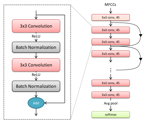
Fig. 1: Our full architecture, with a magnified residual block.

Our architecture is similar to that of He et al. [2], who postulated that it may be easier to learn residuals than to learn the original mapping for deep convolutional neural networks. They found that additional layers in deep networks cannot be merely “tacked on” to shallower nets. Specifically, He et al. proposed that it may be easier to learn the residual $H(\mathbf{x})=F(\mathbf{x})+\mathbf{x}$ instead of the true mapping $F(\mathbf{x})$, since it is empirically difficult to learn the identity mapping for $F$ when the model has unnecessary depth. In residual networks (ResNets), residuals are expressed via connections between layers (see Figure 1), where an input $\mathbf{x}$ to layer $i$ is added to the output of some downstream layer $i+k$, enforcing the residual definition $H(\mathbf{x})=F(\mathbf{x})+\mathbf{x}$.

Following standard ResNet architectures, our residual block begins with a bias-free convolution layer with weights $\mathbf{W}\in\mathbb{R}^{(m\times r)\times n}$, where $m$ and $r$ are the width and height, respectively, and $n$ the number of feature maps. After the convolution layer, there are ReLU activation units and—instead of dropout—a batch normalization [11] layer. In addition to using residual blocks, we also use a $(d_{w},d_{h})$ convolution dilation [12] to increase the receptive field of the network, which allows us to consider the one-second input in its entirety using a smaller number of layers. To expand our input for the residual blocks, which requires inputs and outputs of equal size throughout, our entire architecture starts with a convolution layer with weights $\mathbf{W}\in\mathbb{R}^{(m\times r)\times n}$. A separate non-residual convolution layer and batch normalization layer are further appended to the chain of residual blocks, as shown in Figure 1 and Table 1.

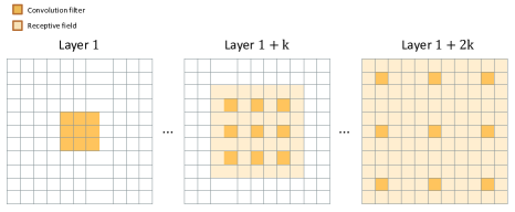
Fig. 2: Exponentially increasing dilated convolutions; in this case, $k=1$.

type	$m$	$r$	$n$	$d_{w}$	$d_{h}$	Par.	Mult.
conv	3	3	45	-	-	405	1.52M
res $\times$ 6	3	3	45	$2^{\lfloor\frac{i}{3}\rfloor}$	$2^{\lfloor\frac{i}{3}\rfloor}$	219K	824M
conv	3	3	45	16	16	18.2K	68.6M
bn	-	-	45	-	-	-	169K
avg-pool	-	-	45	-	-	-	45
softmax	-	-	12	-	-	540	540
Total	-	-	-	-	-	238K	894M

Table 1: Parameters used for res15, along with the number of parameters and multiplies.

Our base model, which we refer to as res15, comprises six such residual blocks and $n=45$ feature maps (see Figure 1). For dilation, as illustrated in Figure 2, an exponential sizing schedule [12] is used: at layer $i$, the dilation is $d_{w}=d_{h}=2^{\lfloor\frac{i}{3}\rfloor}$, resulting in a total receptive field of $125\times 125$. As is standard in ResNet architectures, all output is zero-padded at each layer and finally average-pooled and fed into a fully-connected softmax layer. Following previous work, we measure the “footprint” of a model in terms of two quantities: the number of parameters in the model and the number of multiplies that are required for a full feedforward inference pass. Our architecture uses roughly 238K parameters and 894M multiplies (see Table 1 for the exact breakdown).

type	$m$	$r$	$n$	Par.	Mult.
conv	3	3	19	171	643K
avg-pool	4	3	19	-	6.18K
res $\times$ 3	3	3	19	19.5K	5.0M
avg-pool	-	-	19	-	19
softmax	-	-	12	228	228
Total	-	-	-	19.9K	5.65M

Table 2: Parameters used for res8-narrow.

type	$m$	$r$	$n$	Par.	Mult.
conv	3	3	45	405	1.80M
avg-pool	2	2	45	-	45K
res $\times$ 12	3	3	45	437K	378M
avg-pool	-	-	45	-	45
softmax	-	-	12	540	540
Total	-	-	-	438K	380M

Table 3: Parameters used for res26.

To derive a compact small-footprint model, one simple approach is to reduce the depth of the network. We tried cutting the number of residual blocks in half to three, yielding a model we call res8. Because the footprint of res15 arises from its width as well as its depth, the compact model adds a $4\times 3$ average-pooling layer after the first convolutional layer, reducing the size of the time and frequency dimensions by a factor of four and three, respectively. Since the average pooling layer sufficiently reduces the input dimension, we did not use dilated convolutions in this variant.

In the opposite direction, we explored the effects of deeper models. We constructed a model with double the number of residual blocks (12) with 26 layers, which we refer to as res26. To make training tractable, we prepend a $2\times 2$ average-pooling layer to the chain of residual blocks. Dilation is also not used, since the receptive field of 25 3$\times$3 convolution filters is large enough to cover our input size.

In addition to depth, we also varied model width. All models described above used $n=45$ feature maps, but we also considered variants with $n=19$ feature maps, denoted by -narrow appended to the base model’s name. A detailed breakdown of the footprint of res8-narrow, our best compact model, is shown in Table 2; the same analysis for our deepest and widest model, res26, is shown in Table 3.

4 Evaluation

4.1 Experimental Setup

We evaluated our models using Google’s Speech Commands Dataset [9], which was released in August 2017 under a Creative Commons license. The dataset contains 65,000 one-second long utterances of 30 short words by thousands of different people, as well as background noise samples such as pink noise, white noise, and human-made sounds. The blog post announcing the data release also references Google’s TensorFlow implementation of Sainath and Parada’s models, which provide the basis of our comparisons.

Following Google’s implementation, our task is to discriminate among 12 classes: “yes,” “no,” “up,” “down,” “left,” “right,” “on,” “off,” “stop,” “go”, unknown, or silence. Our experiments followed exactly the same procedure as the TensorFlow reference. The Speech Commands Dataset was split into training, validation, and test sets, with 80% training, 10% validation, and 10% test. This results in roughly 22,000 examples for training and 2,700 each for validation and testing. For consistency across runs, the SHA1-hashed name of the audio file from the dataset determines the split.

To generate training data, we followed Google’s preprocessing procedure by adding background noise to each sample with a probability of $0.8$ at every epoch, where the noise is chosen randomly from the background noises provided in the dataset. Our implementation also performs a random time-shift of $Y$ milliseconds before transforming the audio into MFCCs, where $Y\sim\textsc{Uniform}[-100,100]$. In order to accelerate the training process, all preprocessed inputs are cached for reuse across different training epochs. At each epoch, 30% of the cache is evicted.

Accuracy is our main metric of quality, which is simply measured as the fraction of classification decisions that are correct. For each instance, the model outputs its most likely prediction, and is not given the option of “don’t know”. We also plot receiver operating characteristic (ROC) curves, where the $x$ and $y$ axes show false alarm rate (FAR) and false reject rate (FRR), respectively. For a given sensitivity threshold—defined as the minimum probability at which a class is considered positive during evaluation—FAR and FRR represent the probabilities of obtaining false positives and false negatives, respectively. By sweeping the sensitivity interval $[0.0,1.0]$, curves for each of the keywords are computed and then averaged vertically to produce the overall curve for a particular model. Curves with less area under the curve (AUC) are better.

4.2 Model Training

Mirroring the ResNet paper [2], we used stochastic gradient descent with a momentum of 0.9 and a starting learning rate of 0.1, which is multiplied by 0.1 on plateaus. We also experimented with Nesterov momentum, but we found slightly decreased learning performance in terms of cross entropy loss and test accuracy. We used a mini-batch size of 64 and $L_{2}$ weight decay of $10^{-5}$. Our models were trained for a total of 26 epochs, resulting in roughly 9,000 training steps.

4.3 Results

Model	Test accuracy	Par.	Mult.
trad-fpool3	90.5% $\pm$ 0.297	1.37M	125M
tpool2	91.7% $\pm$ 0.344	1.09M	103M
one-stride1	77.9% $\pm$ 0.715	954K	5.76M
res15	95.8% $\pm$ 0.484	238K	894M
res15-narrow	94.0% $\pm$ 0.516	42.6K	160M
res26	95.2% $\pm$ 0.184	438K	380M
res26-narrow	93.3% $\pm$ 0.377	78.4K	68.5M
res8	94.1% $\pm$ 0.351	110K	30M
res8-narrow	90.1% $\pm$ 0.976	19.9K	5.65M

Table 4: Test accuracy of each model with 95% confidence intervals (across five trials), as well as footprint size in terms of number of parameters and multiplies.

Since our own networks are implemented in PyTorch, we used our PyTorch reimplementations of Sainath and Parada’s models as a point of comparison. We have previously confirmed that our PyTorch implementation achieves the same accuracy as the original TensorFlow reference [10]. Our ResNet models are compared against three CNN variants proposed by Sainath and Parada: trad-fpool3, which is their base model; tpool2, the most accurate variant of those they explored; and one-stride1, their best compact variant. The accuracies of these models are shown in Table 4, which also shows the 95% confidence intervals from five different optimization trials with different random seeds. The table provides the number of model parameters as well as the number of multiplies in an inference pass. We see that tpool2 is indeed the best performing model, slightly better than trad-fpool3. The one-stride1 model substantially reduces the model footprint, but this comes at a steep price in terms of accuracy.

The performance of our ResNet variants is also shown in Table 4. Our base res15 model achieves significantly better accuracy than any of the previous Google CNNs (the confidence intervals do not overlap). This model requires fewer parameters, but more multiplies, however. The “narrow” variant of res15 with fewer feature maps sacrifices accuracy, but remains significantly better than the Google CNNs (although it still uses $\sim$30% more multiplies).

Looking at our compact res8 architecture, we see that the “wide” version strictly dominates all the Google models—it achieves significantly better accuracy with a smaller footprint. The “narrow” variant reduces the footprint even more, albeit with a small degradation in performance compared to tpool2, but requires 50$\times$ fewer model parameters and 18$\times$ fewer multiplies. Both models are far superior to Google’s compact variant, one-stride1.

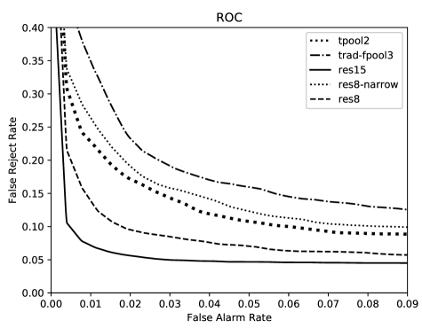
Fig. 3: ROC curves for different models.

Turning our attention to the deeper variants, we see that res26 has lower accuracy than res15, suggesting that we have overstepped the network depth for which we can properly optimize model parameters. Comparing the narrow vs. wide variants overall, it appears that width (the number of feature maps) has a larger impact on accuracy than depth.

We plot the ROC curves of selected models in Figure 3, comparing the two competitive baselines to res8, res8-narrow, and res15. The remaining models were less interesting and thus omitted for clarity. These curves are consistent with the accuracy results presented in Table 4, and we see that res15 dominates the other models in performance at all operating points.

5 Conclusions and Future Work

This paper describes the application of deep residual learning and dilated convolutions to the keyword spotting problem. Our work is enabled by the recent release of Google’s Speech Commands Dataset, which provides a common benchmark for this task. Previously, related work was mostly incomparable because papers relied on private datasets. Our work establishes new, state-of-the-art, open-source reference models on this dataset that we encourage others to build on.

For future work, we plan to compare our CNN-based approaches with an emerging family of models based on recurrent architectures. We have not undertaken such a study because there do not appear to be publicly-available reference implementations of such models, and the lack of a common benchmark makes comparisons difficult. The latter problem has been addressed, and it would be interesting to see how recurrent neural networks stack up against our approach.

References

- [1] Tara N. Sainath and Carolina Parada, “Convolutional neural networks for small-footprint keyword spotting,” in Interspeech, 2015, pp. 1478–1482.
- [2] Kaiming He, Xiangyu Zhang, Shaoqing Ren, and Jian Sun, “Deep residual learning for image recognition,” in CVPR, 2016, pp. 770–778.
- [3] Chunlei Zhang and Kazuhito Koishida, “End-to-end text-independent speaker verification with triplet loss on short utterances,” in Interspeech, 2017, pp. 1487–1491.
- [4] Wayne Xiong, Jasha Droppo, Xuedong Huang, Frank Seide, Mike Seltzer, Andreas Stolcke, Dong Yu, and Geoffrey Zweig, “The Microsoft 2016 conversational speech recognition system,” in ICASSP, 2017, pp. 5255–5259.
- [5] Wayne Xiong, Lingfeng Wu, Fil Alleva, Jasha Droppo, Xuedong Huang, and Andreas Stolcke, “The Microsoft 2017 conversational speech recognition system,” arXiv:1708.06073v2, 2017.
- [6] Guoguo Chen, Carolina Parada, and Georg Heigold, “Small-footprint keyword spotting using deep neural networks,” in ICASSP, 2014, pp. 4087–4091.
- [7] Sercan Ömer Arik, Markus Kliegl, Rewon Child, Joel Hestness, Andrew Gibiansky, Christopher Fougner, Ryan Prenger, and Adam Coates, “Convolutional recurrent neural networks for small-footprint keyword spotting,” arXiv:1703.05390v3, 2017.
- [8] Ming Sun, Anirudh Raju, George Tucker, Sankaran Panchapagesan, Gengshen Fu, Arindam Mandal, Spyros Matsoukas, Nikko Strom, and Shiv Vitaladevuni, “Max-pooling loss training of Long Short-Term Memory networks for small-footprint keyword spotting,” arXiv:1705.02411v1, 2017.
- [9] Pete Warden, “Launching the speech commands dataset,” Google Research Blog, 2017.
- [10] Raphael Tang and Jimmy Lin, “Honk: A PyTorch reimplementation of convolutional neural networks for keyword spotting,” arXiv:1710.06554v2, 2017.
- [11] Sergey Ioffe and Christian Szegedy, “Batch normalization: Accelerating deep network training by reducing internal covariate shift,” arXiv:1502.03167v3, 2015.
- [12] Fisher Yu and Vladlen Koltun, “Multi-scale context aggregation by dilated convolutions,” arXiv:1511.07122v3, 2015.