Multi-level Residual Networks from Dynamical Systems View

Abstract

Deep residual networks (ResNets) and their variants are widely used in many computer vision applications and natural language processing tasks. However, the theoretical principles for designing and training ResNets are still not fully understood. Recently, several points of view have emerged to try to interpret ResNet theoretically, such as unraveled view, unrolled iterative estimation and dynamical systems view. In this paper, we adopt the dynamical systems point of view, and analyze the lesioning properties of ResNet both theoretically and experimentally. Based on these analyses, we additionally propose a novel method for accelerating ResNet training. We apply the proposed method to train ResNets and Wide ResNets for three image classification benchmarks, reducing training time by more than 40% with superior or on-par accuracy.

1 Introduction

Deep neural networks have powered many research areas from computer vision (He et al., 2016; Huang et al., 2017b), natural language processing (Cho et al., 2014) to biology (Esteva et al., 2017) and e-commerce (Ha et al., 2016). Deep Residual Networks (ResNets) (He et al., 2016), and their variants such as Wide ResNets (Zagoruyko & Komodakis, 2016) and DenseNets (Huang et al., 2017b), are among the most successful architectures. In ResNets, the authors employ identity skip-connections that bypass residual layers, allowing data to flow from previous layers directly to any subsequent layers.

With the success of ResNet and its variants on various applications (He et al., 2016; 2017; Pohlen et al., 2017; Xiong et al., 2017; Oord et al., 2016; Wu et al., 2016), several views such as unraveled view (Veit et al., 2016), unrolled iterative estimation view (Greff et al., 2017) and dynamical systems view (Haber et al., 2017; E, 2017; Chang et al., 2017) have emerged to try to interpret ResNets through theoretical analysis and empirical results. These views provide preliminary interpretations, however, deep understanding of ResNets is still an active on-going research topic (Jastrzebski et al., 2017; Li et al., 2016; Hardt & Ma, 2017; Li & Yuan, 2017).

The dynamical systems view interprets ResNets as ordinary differential equations (ODEs), a special kind of dynamical systems (Haber et al., 2017; E, 2017), opening up possibilities of exploiting the computational and theoretical success from dynamical systems to ResNets. From this point of view, stable and reversible architectures (Haber & Ruthotto, 2017; Chang et al., 2017) are developed. However, few empirical analysis of this view has been done and many phenomena such as the removing of layers not leading to performance drop are not explained by the dynamical systems view. In this work, we take steps forward to complement this dynamical systems view with empirical analysis of its properties and the lesion studies.

One challenge of deep ResNets is the long training time. It is extremely time-consuming to train on large datasets such as ImageNet or with very deep ResNets such as 1000-layer networks, which may take several days or even weeks on high-performance hardware with GPU acceleration. Recently the reversible residual networks (Gomez et al., 2017; Chang et al., 2017) consumes 50% more computational time for reducing memory usage by reconstructing the activations, which exposes training time to be a more severe problem. Inspired by the dynamical systems interpretation, we additionally propose a simple yet effective multi-level method for accelerating ResNets training.

In summary, the main contributions of this work are:

• We study the dynamical systems view and explain the lesion studies from this view through empirical analysis.

• We propose a simple yet efficient multi-level training method for ResNets based on dynamical systems view.

• We demonstrate the proposed multi-level training method on ResNets (He et al., 2016) and Wide ResNets (Zagoruyko & Komodakis, 2016) across three widely used datasets, achieving more than 40% training time reduction with superior or on-par accuracy.

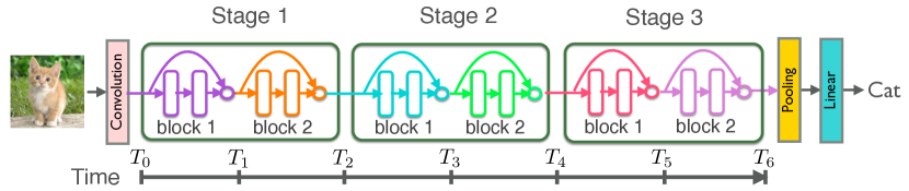
Figure 1: Dynamical systems view of ResNets. ResNets equally discretize the time interval $[0,T]$ using time points $T_{0},T_{1},\ldots,T_{d}$, where $T_{0}=0$, $T_{d}=T$ and $d$ is the total number of blocks.

2 Related work

2.1 ResNets and variants

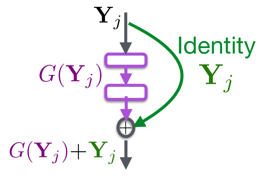
Figure 2: A residual block. Each residual block has two components: the residual module $G$ and the identity skip-connection, which add up to the output of a block.

ResNets (He et al., 2016) are deep neural networks of stacking simple residual blocks, which contain identity skip-connections that bypass the residual layers. A residual block, as shown in Fig. 2, can be written as

$$\mathbf{Y}_{j+1}=\mathbf{Y}_{j}+G(\mathbf{Y}_{j},{\boldsymbol{\theta}}_{j})\quad\mathrm{for}\quad j=0,...,N-1,$$ (1)

where ${\bf Y}_{j}$ is the feature map at the $j$th layer, ${\boldsymbol{\theta}}_{j}$ represents the $j$th layer’s network parameters. $G$ is referred to as a residual module, consisting of two convolutional layers. As shown in Fig. 1, the network is divided into several stages; each consists of a number of residual blocks. In the first block of each stage, the feature map size is halved, and the number of filters is doubled. The feature map remains the same dimensionality for subsequent blocks in a stage.

After the success of ResNets in popular competitions such as ImageNet (Russakovsky et al., 2015), Pascal VOC (Everingham et al., 2010) and Microsoft COCO (Lin et al., 2014), there emerged many successors (Huang et al., 2016; 2017b; Chang et al., 2017; Gomez et al., 2017; Targ et al., 2016; Hardt & Ma, 2017; Zagoruyko & Komodakis, 2016). For instance, DenseNet (Huang et al., 2017b) connects between any two layers with the same feature-map size. ResNxt (Xie et al., 2017) introduces a homogeneous, multi-branch architecture to increase the accuracy.

2.2 Interpretations of ResNets

Unraveled view In Veit et al. (2016), ResNets are interpreted from an unraveled view in which ResNets are viewed as a collection of many paths which data flow along from input to output. Each residual block consists of a residual module and an identity skip-connection; a path is defined as a configuration of which residual module to enter and which to skip. For a ResNet with $n$ residual blocks, there are $2^{n}$ unique paths. Through lesion studies, Veit et al. (2016) further demonstrate that paths in ResNets do not strongly depend on each other and behave like an ensemble. When a residual block is removed, the number of paths is reduced from $2^{n}$ to $2^{n-1}$, leaving half of the paths still valid, which explains why ResNets are resilient to dropping blocks. Besides the explicit ensemble view, training ResNets with stochastic depth (Huang et al., 2016) can be viewed as an ensemble of networks with varying depths implicitly.

Unrolled iterative estimation view ResNets are interpreted as unrolled iterative estimation in Greff et al. (2017). From this view, the level of representation stays the same within each stage. The residual blocks in a stage work together to estimate and iteratively refine a single level of representation: the first layer in a stage provides a rough estimate for the representation, and subsequent layers refine that estimate. An implication of this view is that processing in each block is incremental and removing blocks only has a mild effect on the final results. Based on this view, Jastrzebski et al. (2017) provide more analytical and empirical results.

Dynamical systems view ResNets can be interpreted as a discretization of dynamical systems (Haber et al., 2017; E, 2017). The basic dynamics at each step is a linear transformation followed by component-wise nonlinear activation function. The behavior of large dynamical systems is often a notoriously difficult problem in mathematics, particularly for discrete dynamical systems. This is similar to the gradient exploding/vanishing problem for deep neural networks or recurrent neural networks. Imposing structural constraints on dynamical systems such as Hamiltonian systems to conserve the energy is explored in Haber & Ruthotto (2017); Chang et al. (2017). However, no interpretation on the phenomenon of deleting layers is studied from this point of view.

2.3 ResNets efficient training methods

One major challenge of deep ResNets is their long training time. To alleviate this issue, several attempts have been made. Stochastic depth (Huang et al., 2016) randomly drops entire residual blocks during training and bypassing their transformations through identity skip-connections; during testing, all the blocks are in use. When a block is bypassed for a specific iteration, there is no need to perform forward-backward computation. With stochastic depth, approximately $25\%$ of training time could be saved. Figurnov et al. (2017) reduce the inference time of residual networks by learning to predict early halting scores based on the image content. Huang et al. (2017a) investigate image classification with computational resource limits at test time. SparseNets (Zhu et al., 2018) is a simple feature aggregation structure with shortcut paths bypassing exponentially growing number of layers. Mollifying networks (Gulcehre et al., 2016) start the optimization with an easier (possibly convex) objective function and let it evolve during the training, until it eventually goes back to being the original, difficult to optimize, objective function. It can also be interpreted as a form adaptive noise injection that only depends on a single hyperparameter.

3 ResNets from dynamical systems view

In this section, we first provide a brief introduction to the dynamical systems view in which ResNets are considered as ODEs. Based on this view, we provide empirical analysis to explain some intriguing properties and phenomena of ResNets.

3.1 Dynamical systems view

For the pre-activation ResNets $\mathbf{Y}_{j+1}=\mathbf{Y}_{j}+G(\mathbf{Y}_{j},{\boldsymbol{\theta}}_{j}),$ the residual module $G$ consists of two sets of batch normalization, ReLU and convolutional layers. Without loss of generality, we can conceptually add a parameter $h$ and rewrite the residual module as $G=hF$. The residual block becomes

$$\mathbf{Y}_{j+1}=\mathbf{Y}_{j}+hF(\mathbf{Y}_{j},{\boldsymbol{\theta}}_{j}),$$ (2)

which can be further rewritten as

$$\frac{\mathbf{Y}_{j+1}-\mathbf{Y}_{j}}{h}=F(\mathbf{Y}_{j},{\boldsymbol{\theta}}_{j}).$$ (3)

For a sufficiently small $h$, Eq. (3) can be regarded as a forward Euler discretization of the initial value ODE

$$\dot{\mathbf{Y}}(t)=F(\mathbf{Y}(t),{\boldsymbol{\theta}}(t)),\ \mathbf{Y}(0)=\mathbf{Y}_{0},\ \mathrm{for}\ 0\leq t\leq T,$$ (4)

where time $t$ corresponds to the direction from input to output, $\mathbf{Y}(0)$ is the input feature map after the initial convolution, and $\mathbf{Y}(T)$ is the output feature map before the softmax classifier. Thus, the problem of learning the network parameters, ${\boldsymbol{\theta}}$, is equivalent to solving a parameter estimation problem or optimal control problem involving the ODE in Eq. (4).

3.2 Time step size

The new parameter $h$ is called the step size of discretization. In the original formulation of ResNets in Eq. (1), $h$ does not exist, and is implicitly absorbed by the residual module $G$. We call it the implicit step size. The step size $h$ can also be explicitly expressed in the model: the output of the residual module is multiplied by $h$ before being added to the identity mapping. In this case, $h$ is a hyper-parameter and we name it the explicit step size. In this section, we only consider implicit step size.

We assume that ${\bf Y}(0)$ and ${\bf Y}(T)$ correspond to the input and output feature maps of the network respectively, where the time length $T$ is fixed. As illustrated in Fig. 1, ResNets equally discretize $[0,T]$ using time points $T_{0},T_{1},\ldots,T_{j},\ldots,T_{d}$, where $T_{0}=0$, $T_{d}=T$ and $d$ is the number of blocks. Thus each time step is $h=T_{j+1}-T_{j}=T/d$.

Thus, we can obtain

$$\|G({\bf Y}_{j})\|=\|hF({\bf Y}_{j})\|=\frac{T}{d}\|F({\bf Y}_{j})\|,$$ (5)

where $F$ in the underlying ODE in Eq. (4) does not depend on $d$. In other words, $d$ is inversely proportional to the norm of the residual modules $G(Y_{j})$.

Empirical analysis To verify the above statement, we run experiments on ResNets with varying depths. If our theory is correct, the norm of the residual module $\|G({\bf Y}_{j})\|$ should be inversely proportional to the number of residual blocks. Take ResNet-32 with 15 residual blocks in total as an example. We calculate the average $L^{2}$-norm of the residual modules $\gamma=\frac{1}{15}\sum_{j=1}^{15}\|G(\mathbf{Y}_{j})\|$. Figure 3 shows $\gamma$ for different ResNet models. The curve resembles a reciprocal function, which is consistent with Eq. (5) and the dynamical system point of view.

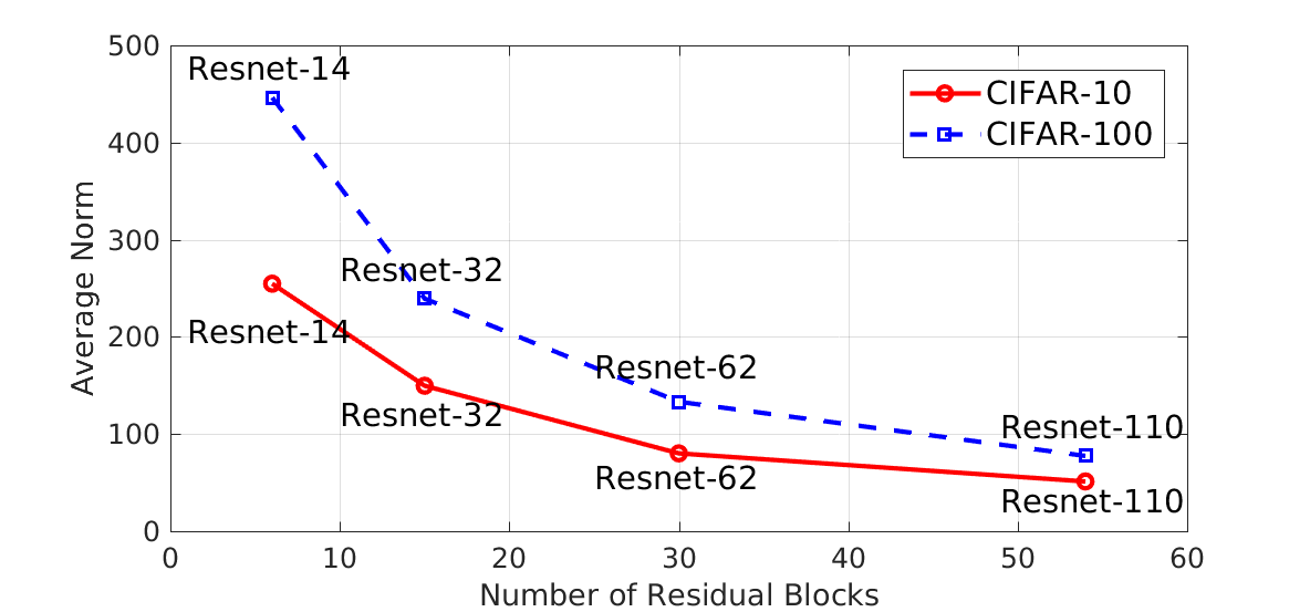
Figure 3: The average $L^{2}$-norm of the residual modules $\gamma$ vs the number of residual blocks $d$. The curve resembles a reciprocal function, which is consistent with Eq. (5) and the dynamical systems view.

3.3 Lesion study

Lesion studies for ResNets in Veit et al. (2016) remove single or multiple residual blocks, and shuffle the residual blocks at test time. Surprisingly, only removing downsampling blocks has a modest impact on performance, no other block removal leads to a noticeable effect.

According to the dynamical systems view, removing one residual block is equivalent to skipping one time step and squeezing two adjacent steps into one. This operation may change the dynamical system. However, we will show in the following that the effect is negligible when the output of residual module $G({\bf Y}_{j})$ is small enough.

Let $t_{0},t_{1},t_{2}$ be three consecutive time points such that $t_{1}=t_{0}+h$ and $t_{2}=t_{0}+2h$. Suppose the removed block corresponds to time point $t_{1}$. Before the removal of the time point, the discretization is

$${\bf Y}(t_{1}) ={\bf Y}(t_{0})+hF({\bf Y}(t_{0})),$$

$${\bf Y}(t_{2}) ={\bf Y}(t_{1})+hF({\bf Y}(t_{1}))={\bf Y}(t_{0})+hF({\bf Y}(t_{0}))+hF({\bf Y}(t_{1})).$$ (6)

After $t_{1}$ is removed, the time interval $[t_{0},t_{2}]$ is squeezed to $[t_{0},t_{2}^{\prime}]$, where $t_{2}^{\prime}=t_{0}+h$ is the new time point after $t_{0}$. The new discretization is

$${\bf Y}(t_{2}^{\prime})={\bf Y}(t_{0})+hF({\bf Y}(t_{0})).$$ (7)

The difference of the feature before and after the removal operation is

$${\bf Y}(t_{2}^{\prime})-{\bf Y}(t_{2})=hF({\bf Y}(t_{1})),$$ (8)

which is the output of the residual module $G({\bf Y}(t_{1}))$. Therefore, the effect of removing the block is negligible when $G({\bf Y}(t_{1}))$ is small.

Empirical analysis To empirically verify that $G({\bf Y}(t))$ are small, we train a ResNet-110 model (3 stages with 18 residual blocks per stage) on CIFAR-10/100, and plot the $L^{2}$-norm of input ${\bf Y}_{j}$ and output $G({\bf Y}_{j})$ of each residual module at test time. As shown in Figure 4, except for the first block at each stage, later blocks have tiny residual module outputs $G({\bf Y}_{j})$ compared with the inputs ${\bf Y}_{j}$. This provides an explanation why removing one block does not notably impact the performance.

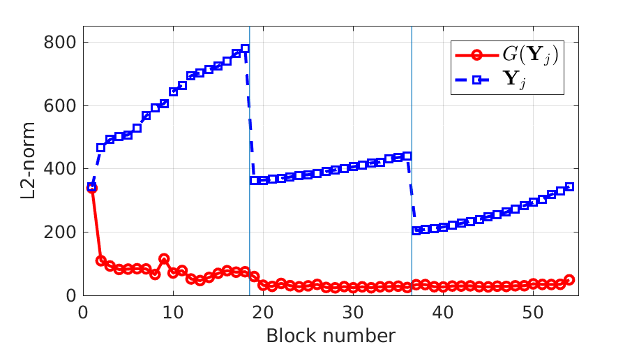
(a) CIFAR-10

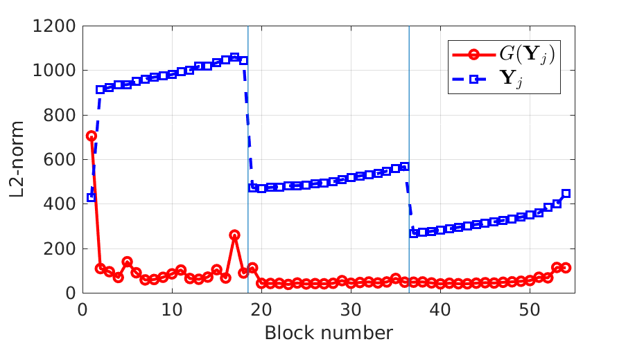
(b) CIFAR-100

Figure 4: $L^{2}$-norm of the input and output of the residual module $G$. ResNet-110 models are trained on CIFAR-10 and CIFAR-100. The norms are evaluated at test time. It shows that within a residual block, the identity mapping contributes much more than the residual module. In other words, $G({\bf Y}_{j})$ is relatively small for most residual blocks.

The effect of shuffling residual blocks can be analyzed in a similar way. When the outputs of the residual modules are small, each block only slightly modifies the feature map. Therefore, we can expect the effect of shuffling to be moderate, especially in later stages.

When the network is deep, the outputs of the residual modules are close to zero. Each residual module can be regarded as feature refinement. The magnitude of change is large only in the first block; the subsequent blocks only slightly refine the features, which is consistent with the unrolled iterative estimation view.

4 Efficient training with multi-level method

Given the connection between ResNets and ODEs, existing theories and numerical techniques for ODEs can be applied to ResNets. In numerical analysis, multi-grid methods (Hackbusch, 2013) are algorithms for solving differential equations using a hierarchy of discretizations with varying step sizes. Inspired by multi-grid methods, we propose the multi-level training method.

4.1 Multi-level training

The idea of the multi-level method is, during training, we start with a shallow network using a large explicit step size $h$. After a few training steps, we switch to a deeper network, by doubling the number of residual blocks and halving the step size to $h/2$. This operation is called interpolation, which applies to all the stages at the same time. Fig. 5 illustrates the interpolation operation for one stage. The interpolation operation inserts a new residual block right after every existing block, and copies the convolutional weights and batch normalization parameters from the adjacent old block to the new block.

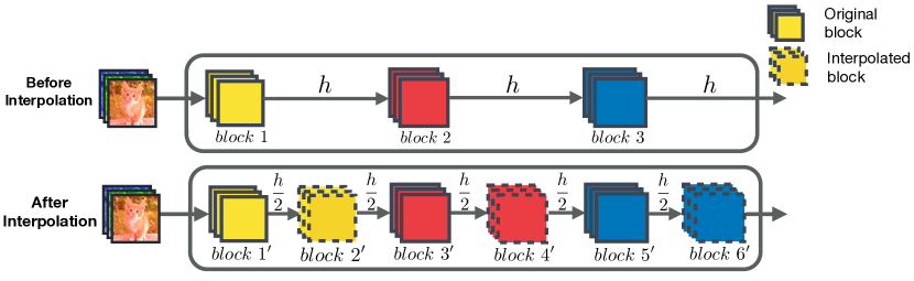
Figure 5: An illustration of the interpolation operation for one stage. We insert one residual block right after each existing block in the stage. The model parameters, including convolutional weights and batch normalization parameters, are copied from the adjacent old block to interpolated blocks. After that, the explicit step size $h$ is halved. For example, before interpolation, this stage has three residual blocks, numbered 1 to 3. After interpolation, block 1, 2 and 3 become block 1’, 3’ and 5’ respectively. Three new blocks are inserted: block 2’, 4’ and 6’, whose parameters are copied from its previous block respectively.

In the multi-level training process, interpolations happen several times, thus dividing the training steps into cycles. Table 1 gives an example to illustrate this process. According to our dynamical systems view, by interpolating the residual blocks and halving the step size, we solve exactly the same differential equation. Therefore, the interpolation operation at the beginning of a cycle gives a good initialization of the parameters.

	# Residual Blocks	Explicit Step Size $h$	# Training Steps
Cycle 1	2-2-2	1	$N_{1}$
Cycle 2	4-4-4	0.5	$N_{2}$
Cycle 3	8-8-8	0.25	$N_{3}$

Table 1: An illustration of the multi-level method with 3 cycles. The ResNet model has 3 stages; # Residual Blocks column represents the number of blocks in each stage. In cycle 1, the training starts with a 2-2-2 model using $h=1$. After $N_{1}$ training steps, the first interpolation happens: the model becomes 4-4-4, and the step size is halved to $0.5$. Similarly, $N_{2}$ training steps later, the second interpolation doubles the number of blocks to 8-8-8 and halves $h$ to 0.25. Cycle 3 lasts for $N_{3}$ training steps.

Each cycle itself can be regarded as a training process, thus we need to reset the learning rate to a large value at the beginning of each training cycle and anneal the learning rate during that cycle. Here we adopt the cosine annealing learning rate schedule (Loshchilov & Hutter, 2017). Within each cycle, the learning rate is

$$\eta=\eta_{\min}+\frac{1}{2}(\eta_{\max}-\eta_{\min})(1+\cos(\frac{T_{\mathrm{cur}}}{T}\pi)),$$ (9)

where $\eta_{\min}$ and $\eta_{\max}$ represent the minimum and maximum learning rate respectively, $T_{\mathrm{cur}}$ accounts for how many training steps have been performed in the current cycle, and $T$ denotes the total number of training steps in this cycle. The learning rate starts from $\eta_{\max}$ at the beginning of each cycle and decreases to $\eta_{\min}$ at the end of the cycle.

4.2 Training time

# Interpolations	0	1	2	3	4	5	$\cdots$
Theoretical Time Saved	0%	$25\%$	$42\%$	$53\%$	$61\%$	67%	$\cdots$

Table 2: Number of interpolations vs theoretical time saved, relative to the full model. Theoretically, time saved is monotonically increasing as the number of interpolation increases, but the marginal benefit is diminishing.

Since the number of residual blocks in cycle $i$ is half of that in cycle $i+1$, theoretically, the running time in cycle $i$ should also be half of that in cycle $i+1$. Take a multi-level method with two cycles as an example, it trains a shallow model (2-2-2 blocks) for $N$ steps and switches to a deep model (4-4-4 blocks) for another $N$ steps. Compared with the deep model trained for $2N$ steps, the multi-level method reduces training time by $1/4$.

More generally, if one uses the multi-level method with $k$ interpolations equally dividing the training steps, theoretically it saves $1-\frac{2^{k+1}-1}{2^{k}(k+1)}$ of training time, compared to the full model (model in the last cycle) trained for the same number of total steps. Table 2 shows the theoretical time saved. Time saved is monotonically increasing as the number of interpolation increases, but the marginal time saved is diminishing. Furthermore, when the number of interpolations is large, each cycle might not have enough training steps. Therefore, there is a trade-off between efficiency and accuracy.

5 Experiments

The empirical results on the dynamical systems view are presented in Sec. 3.2 and 3.3. In this section, we evaluate the efficacy and efficiency of the proposed multi-level method on two state-of-the art deep learning architectures for image classification: ResNet and Wide ResNet, across three standard benchmarks.

Model	# Blocks	CIFAR-10		CIFAR-100		STL-10
		Error	Time	Error	Time	Error	Time
ResNet-14	2-2-2	9.75%	38m	33.34%	38m	27.78%	33m
ResNet-50	8-8-8	7.58%	114m	28.64%	115m	25.95%	114m
ResNet-50-i (Ours)	2-2-2 to 8-8-8	7.10%	67m	28.71%	68m	25.98%	68m
ResNet-32	5-5-5	7.74%	76m	29.96%	74m	26.02%	71m
ResNet-122	20-20-20	6.47%	266m	26.74%	266m	25.16%	266m
ResNet-122-i (Ours)	5-5-5 to 20-20-20	6.56%	154m	26.81%	154m	24.36%	162m

Table 3: Main multi-level method results for ResNets with different depths. The model name with $i$ corresponds to the multi-level method. Our multi-level training method achieves superior or on-par accuracy with the last cycle model while saving about $40\%$ of training time. The unit of training time is a minute.

5.1 Datasets and networks

Datasets Three widely used datasets are used for evaluation: CIFAR-10, CIFAR-100 (Krizhevsky & Hinton, 2009), and STL10 (Coates et al., 2011). Details on these datasets and data augmentation methods can be found in Appendix A.

Networks We use ResNets (He et al., 2016) and Wide ResNets (Zagoruyko & Komodakis, 2016) for all the datasets. All the networks have three stages, with the number of filters equal to 16-32-64 for ResNets, and 32-64-128 for Wide ResNets.

5.2 Experimental settings

Based on the analysis in Table 2, we use two interpolations, that is three cycles, for the multi-level method in order to optimize the trade-off between efficiency and accuracy.

For each experiment, we run our multi-level model with three cycles. For comparison, two other models are trained for the same number of steps: a model with the same architecture as the first cycle and a model with the same architecture as the last cycle.

We call them first cycle model and last cycle model respectively. We also use the cyclic learning rate schedule (Loshchilov & Hutter, 2017) for the first cycle model and last cycle model for fair comparison.

All the models are trained for 160 epochs. For our multi-level method, the models are interpolated at the 60th and 110th epochs. For baseline models, the learning rate cycle also restarts at epoch 60 and 110. The maximum and minimum learning rates $\eta_{\min}$ and $\eta_{\max}$ are set $0.001$ and $0.5$ respectively. For CIFAR-10 and CIFAR-100 experiments, the mini-batch size is 100. For STL-10 experiments, the mini-batch size is 32. We use a weight decay of $2\times 10^{-4}$, and momentum of $0.9$. All the experiments are evaluated on machines with a single Nvidia GeForce GTX 1080 GPU. The networks are implemented using TensorFlow library (Abadi et al., 2016).

5.3 Main results and analysis

We present the main results and analysis in this section. More experimental results can be found in Appendix D. The theoretical time saved for two interpolations is $42\%$, which is consistent with the experiment results.

The main results are shown in Table 3 and 4, for ResNets and Wide ResNets respectively. We report the test error rate and training time. Compared with the first cycle model, our multi-level method achieves much lower test error. Compared with the last cycle model, the test error is competitive or slightly lower, but the training time reduction is over $40\%$. This result applies to both ResNets and WResNets across three datasets. The interpolation of (Wide) ResNet-50-i from $2$-$2$-$2$ to $8$-$8$-$8$ and (Wide) ResNet-122-i from $5$-$5$-$5$ to $20$-$20$-$20$ show that our multi-level training method is effective for different network depths.

The train and test curves with both ResNets and Wide ResNets are shown in Fig. 6. Although both training and test accuracy temporarily drops at the start of each cycle, the performance eventually surpasses the previous cycles. ResNets and Wide ResNets have similar train and test curves, indicating that our multi-level training method is effective for different network widths.

Model	# Blocks	CIFAR-10		CIFAR-100		STL-10
		Error	Time	Error	Time	Error	Time
WResNet-14	2-2-2	7.38%	51m	27.92%	51m	24.58%	63m
WResNet-50	8-8-8	5.87%	174m	24.49%	173m	23.82%	222m
WResNet-50-i (Ours)	2-2-2 to 8-8-8	5.95%	101m	24.92%	101m	22.82%	131m
WResNet-32	5-5-5	6.29%	111m	25.32%	111m	23.51%	136m
WResNet-122	20-20-20	5.38%	406m	23.11%	406m	22.00%	516m
WResNet-122-i (Ours)	5-5-5 to 20-20-20	5.46%	239m	23.04%	237m	22.65%	307m

Table 4: Main multi-level method results for Wide ResNets (WResNets) with different depths. The model name with $i$ corresponds to the multi-level method. Our multi-level training method achieves superior or on-par accuracy with the last cycle model while saving about $40\%$ of training time. The unit of training time is a minute.

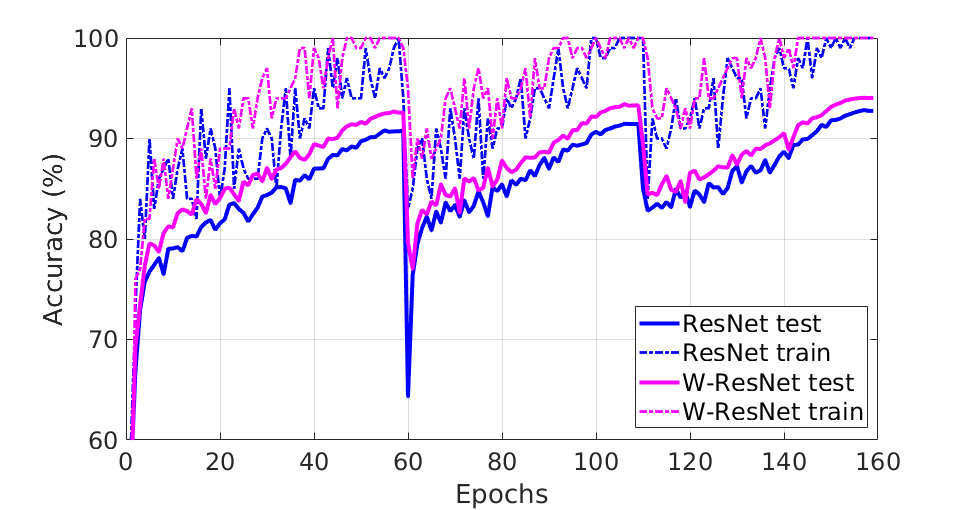
(a) CIFAR-10

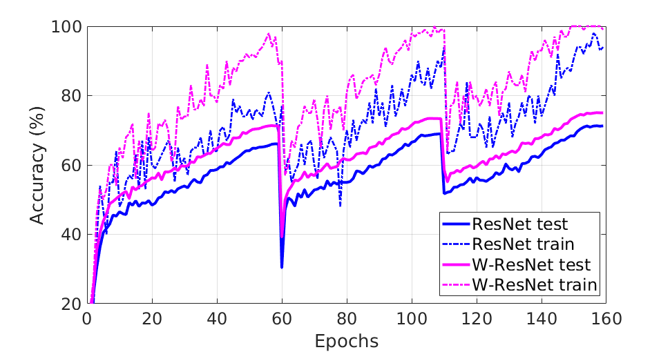
(b) CIFAR-100

Figure 6: Train and test curves using our multi-level method with ResNet-50-i and WResNet-50-i on CIFAR-10/100. The models are interpolated at epoch 60 and 110, dividing the training steps to three cycles. Although both training and test accuracy temporarily drops at the start of each cycle, the performance eventually surpasses the previous cycles.

6 Conclusion

In this work, we study ResNets from the dynamical systems view and explain the lesion studies from this view through both theoretical and empirical analyses. Based on these analyses, we develop a simple yet effective multi-level method for accelerating the training of ResNets. The proposed multi-level training method is evaluated on two state-of-the-art residual network architectures across three widely used classification benchmarks, reducing training time by more than $40\%$ with similar accuracy. For future work, we would like to explore the dynamical systems view on other ResNets variants such as DenseNets.

Appendix A Datasets and model details

CIFAR-10 and CIFAR-100 The CIFAR-10 dataset (Krizhevsky & Hinton, 2009) consists of 50,000 training images and 10,000 testing images in 10 classes with $32\times 32$ image resolution. The CIFAR-100 dataset has the same number of training and testing images as CIFAR-10, but has 100 classes. We use the common data augmentation techniques including padding four zeros around the image, random cropping, random horizontal flipping and image standardization (Huang et al., 2016).

STL-10 The STL-10 dataset (Coates et al., 2011) is an image classification dataset with 10 classes with image resolutions of $96\times 96$. It contains 5,000 training images and 8,000 testing images. Compared with CIFAR-10/100, each class has fewer training samples but higher image resolution. We use the same data augmentation as the CIFAR-10/100 except for padding $12$ zeros around the images.

Number of parameters We list the number of parameters for each model in Table 5.

Model	# Blocks	CIFAR-10	CIFAR-100	STL-10
ResNet-14	2-2-2	172,506	178,356	172,506
ResNet-50	8-8-8	755,802	761,652	755,802
ResNet-32	5-5-5	464,154	470,004	464,154
ResNet-122	20-20-20	19,22,394	1,928,244	19,22,394
WResNet-14	2-2-2	685,994	697,604	685,994
WResNet-50	8-8-8	3,013,802	3,025,412	3,013,802
WResNet-32	5-5-5	1,849,898	1,861,508	1,849,898
ResNet-122	20-20-20	7,669,418	7,681,028	7,669,418

Table 5: The number of parameters for each network model.

Appendix B Implementation details

Interpolation Figure 5 gives a conceptual illustration of the interpolation operation. When implementing this operation, the first block in each stage requires special treatment. The first block changes the size of the feature map and the number of channels, thus the shapes of convolution and batch normalization parameters are different from those in subsequent blocks. As a result, we cannot simply copy the parameters from block 1’ to block 2’. Instead, the parameters of block 2’ are copied from block 3’.

Appendix C Further analysis of time step size

Instead of using $h$ as an implicit step size in Sec. 3.2, we can also explicitly express it in the model. That is, a residual block represents the function $F$ instead of $G$, and $h$ becomes a hyperparameter of the model. In other words, in each residual block, the output of the residual module is multiplied by $h$ before being added to the identity mapping. Now $h$ is the explicit step size that we can control. This enables us to verify the claim that the depth of the network does not affect the underlying differential equation.

Empirical analysis We run the following experiments on CIFAR-10 and CIFAR-100:

• ResNet-32: 15 blocks with $h=1$;

• ResNet-62: 30 blocks with $h=0.5$;

• ResNet-122: 60 blocks with $h=0.25$;

According to our theory, those three models are different discretizations of the same differential equation in Eq. (2). As a result, the function values $F(t)$ should be roughly the same across the time interval $[0,T]$, which is discretized to 15, 30 and 60 time steps respectively. In Figure 7, we plot the $L^{2}$-norm of the residual blocks $F({\bf Y}_{j})$ and scale the block number to the corresponding conceptual time points. It can be seen from the figure that the three curves follow the same trend, which represents the underlying function $F(t)$.

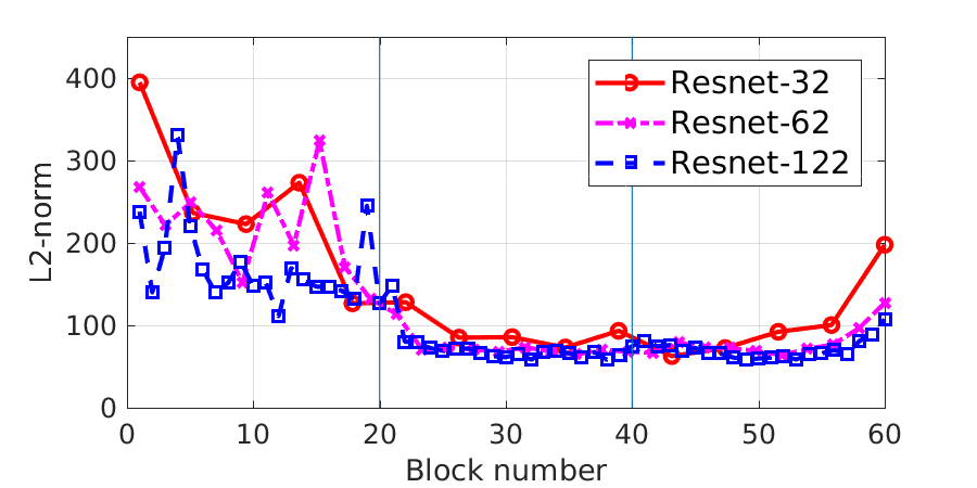
(a) CIFAR-10

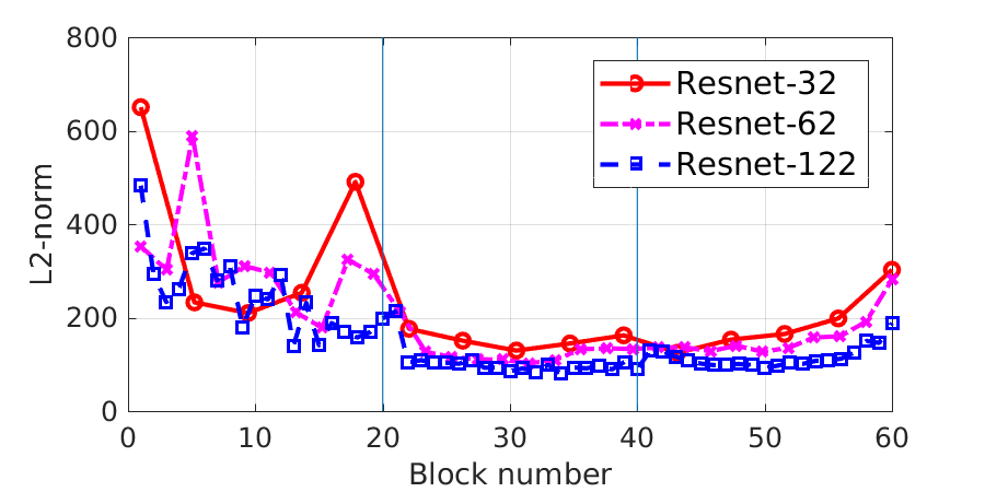
(b) CIFAR-100

Figure 7: Comparison of $\|F({\bf Y}_{j})\|$ among three models: (1) ResNet-32 with $h=1$, (2) ResNet-62 with $h=0.5$, (3) ResNet-122 with $h=0.25$. If the dynamical systems view is correct, the three curves should approximately follow the same trend.

Appendix D More experimental results

Train and test curves on STL-10 We show the train and test curves using our multi-level training method on ResNet-50-i and Wide ResNet-50-i on STL10 in Fig. 8.

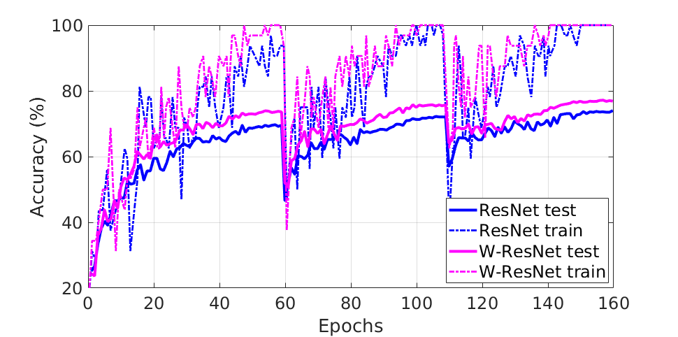
Figure 8: Train and test curves using our multi-level method with ResNet-50-i and WResNet-50-i on STL10. Although both training and testing accuracy temporarily drops at the start of each cycle, the performance eventually surpasses the previous cycles.

Effect of learning rate To study the effect of $\eta_{\max}$ and $\eta_{\min}$ on the cyclic learning rate in Eq. (9), we plot their effect on test accuracy in Fig. 9. We empirically find that $\eta_{\max}=0.5$ and $\eta_{\min}=0.001$ achieve the best accuracy. With the increase of maximum learning rate $\eta_{\max}$, the test accuracy increases first and then decreases. A potential explanation is that with a small learning rate, the system learns slowly, while with a high learning rate, the system contains too much kinetic energy and is unable to reach the deeper and narrower parts of the loss function.

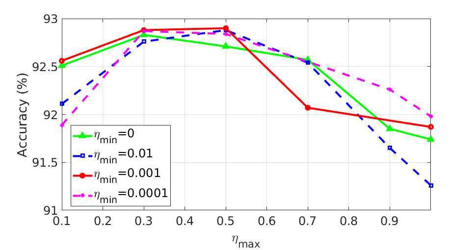
Figure 9: Effect of $\eta_{\max}$ and $\eta_{\min}$ in cyclic learning rate. In most cases, as $\eta_{\max}$ increases, the testing accuracy increases first and then decreases.

Effect of resetting the learning rate To study the effect of resetting the learning rate at the beginning of each cycle, we also run the multi-level training method without resetting the learning rate, that is to use Eq. 9 throughout all cycles. The experiment setting is the same as described in Section 5.2. We train Resnet-50-i on CIFAR-10, CIFAR-100 and STL-10. Each setting is repeated 10 times to obtain the confidence intervals. Fig. 10 shows the results: resetting the learning rate at the beginning of each cycle gives better validation accuracy.

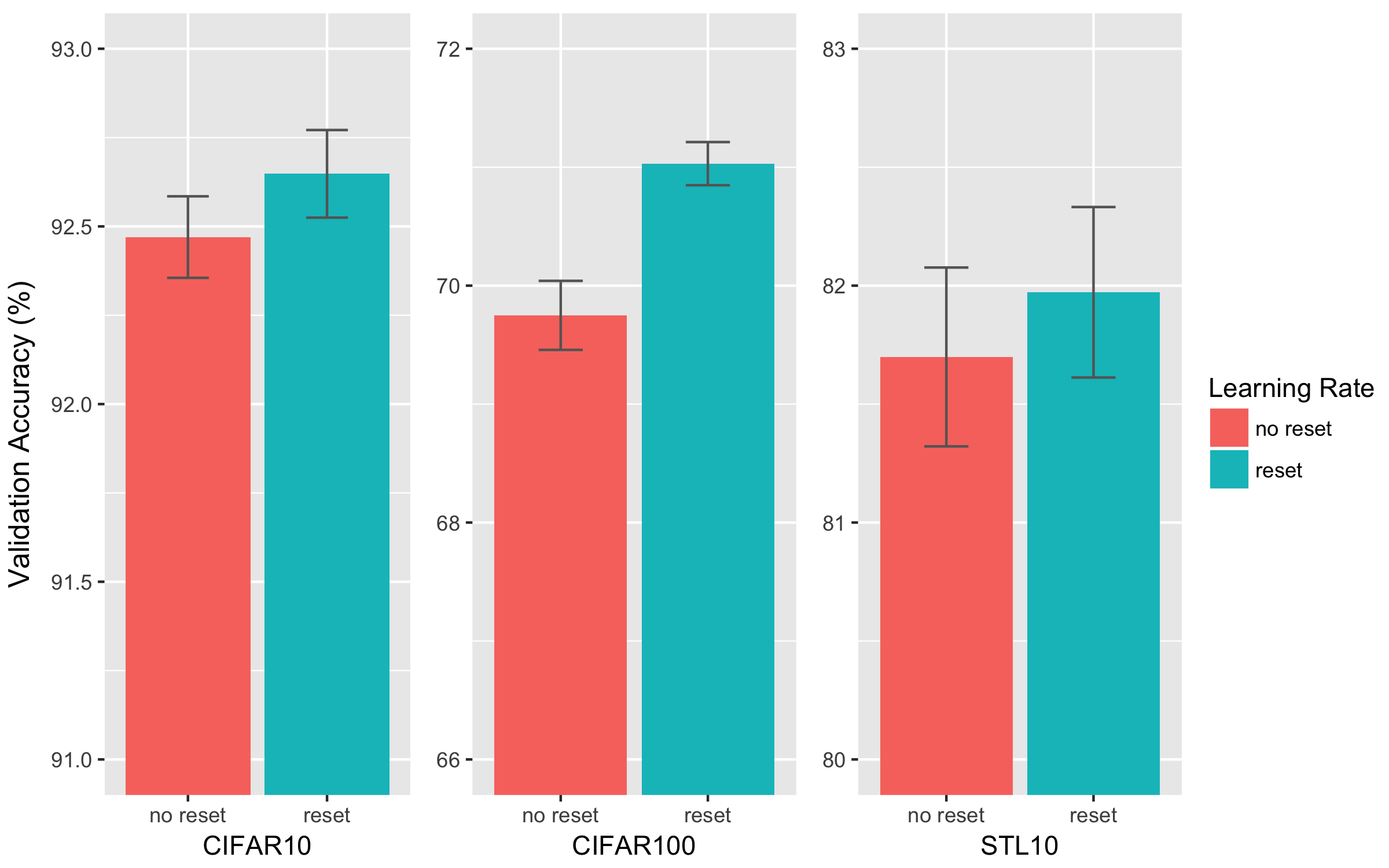
Figure 10: Effect of resetting the learning rate. Resetting the learning rate at the beginning of each cycle gives better validation accuracy.

Comparison with shallow and deep ResNets Fig. 11 shows that training accuracy curves for a shallow ResNet (same depth as the starting model) and a deep ResNet (same depth as the final model).

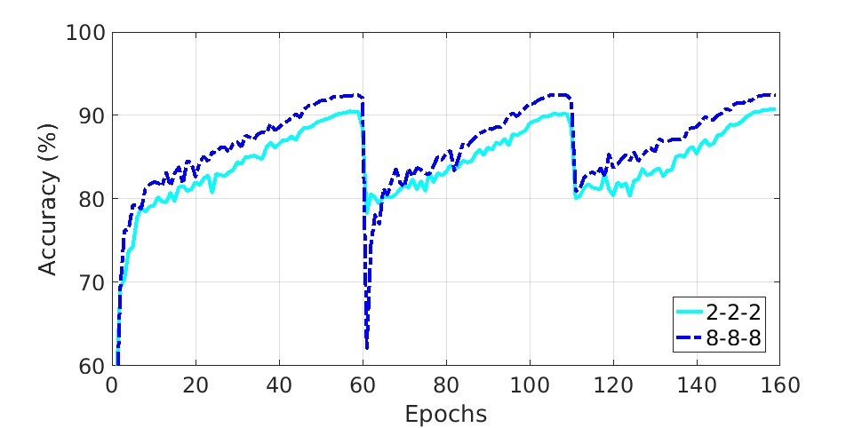
(a) CIFAR-10

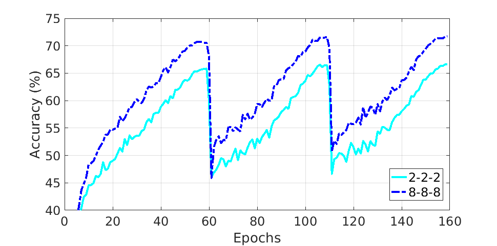
(b) CIFAR-100

Figure 11: Shallow and deep ResNets. Training accuracy curves for a shallow ResNet (same depth as the starting model) and a deep ResNet (same depth as the final model).

References

- Abadi et al. (2016) Martín Abadi, Ashish Agarwal, Paul Barham, Eugene Brevdo, Zhifeng Chen, Craig Citro, Greg S Corrado, Andy Davis, Jeffrey Dean, Matthieu Devin, et al. Tensorflow: Large-scale machine learning on heterogeneous distributed systems. arXiv preprint arXiv:1603.04467, 2016.
- Chang et al. (2017) Bo Chang, Lili Meng, Eldad Haber, Lars Ruthotto, David Begert, and Elliot Holtham. Reversible architectures for arbitrarily deep residual neural networks. arXiv preprint arXiv:1709.03698, 2017.
- Cho et al. (2014) Kyunghyun Cho, Bart Van Merriënboer, Caglar Gulcehre, Dzmitry Bahdanau, Fethi Bougares, Holger Schwenk, and Yoshua Bengio. Learning phrase representations using rnn encoder-decoder for statistical machine translation. ACL, 2014.
- Coates et al. (2011) Adam Coates, Andrew Ng, and Honglak Lee. An analysis of single-layer networks in unsupervised feature learning. In Proceedings of the fourteenth international conference on artificial intelligence and statistics, 2011.
- E (2017) Weinan E. A proposal on machine learning via dynamical systems. Communications in Mathematics and Statistics, 5(1):1–11, 3 2017.
- Esteva et al. (2017) Andre Esteva, Brett Kuprel, Roberto A Novoa, Justin Ko, Susan M Swetter, Helen M Blau, and Sebastian Thrun. Dermatologist-level classification of skin cancer with deep neural networks. Nature, 2017.
- Everingham et al. (2010) Mark Everingham, Luc Van Gool, Christopher KI Williams, John Winn, and Andrew Zisserman. The pascal visual object classes (voc) challenge. IJCV, 2010.
- Figurnov et al. (2017) Michael Figurnov, Maxwell D Collins, Yukun Zhu, Li Zhang, Jonathan Huang, Dmitry Vetrov, and Ruslan Salakhutdinov. Spatially adaptive computation time for residual networks. CVPR, 2017.
- Gomez et al. (2017) Aidan N Gomez, Mengye Ren, Raquel Urtasun, and Roger B Grosse. The reversible residual network: Backpropagation without storing activations. NIPS, 2017.
- Greff et al. (2017) Klaus Greff, Rupesh K Srivastava, and Jürgen Schmidhuber. Highway and residual networks learn unrolled iterative estimation. In ICLR, 2017.
- Gulcehre et al. (2016) Caglar Gulcehre, Marcin Moczulski, Francesco Visin, and Yoshua Bengio. Mollifying networks. arXiv preprint arXiv:1608.04980, 2016.
- Ha et al. (2016) Jung-Woo Ha, Hyuna Pyo, and Jeonghee Kim. Large-scale item categorization in e-commerce using multiple recurrent neural networks. In KDD, 2016.
- Haber & Ruthotto (2017) Eldad Haber and Lars Ruthotto. Stable architectures for deep neural networks. arXiv preprint arXiv:1705.03341, 2017.
- Haber et al. (2017) Eldad Haber, Lars Ruthotto, and Elliot Holtham. Learning across scales-a multiscale method for convolution neural networks. arXiv preprint arXiv:1703.02009, 2017.
- Hackbusch (2013) Wolfgang Hackbusch. Multi-grid methods and applications, volume 4. Springer Science & Business Media, 2013.
- Hardt & Ma (2017) Moritz Hardt and Tengyu Ma. Identity matters in deep learning. ICLR, 2017.
- He et al. (2016) Kaiming He, Xiangyu Zhang, Shaoqing Ren, and Jian Sun. Deep residual learning for image recognition. In CVPR, 2016.
- He et al. (2017) Kaiming He, Georgia Gkioxari, Piotr Dollár, and Ross Girshick. Mask R-CNN. In ICCV, 2017.
- Huang et al. (2016) Gao Huang, Yu Sun, Zhuang Liu, Daniel Sedra, and Kilian Q Weinberger. Deep networks with stochastic depth. In ECCV, 2016.
- Huang et al. (2017a) Gao Huang, Danlu Chen, Tianhong Li, Felix Wu, Laurens van der Maaten, and Kilian Q Weinberger. Multi-scale dense convolutional networks for efficient prediction. arXiv preprint arXiv:1703.09844, 2017a.
- Huang et al. (2017b) Gao Huang, Zhuang Liu, Kilian Q Weinberger, and Laurens van der Maaten. Densely connected convolutional networks. CVPR, 2017b.
- Jastrzebski et al. (2017) Stanisław Jastrzebski, Devansh Arpit, Nicolas Ballas, Vikas Verma, Tong Che, and Yoshua Bengio. Residual connections encourage iterative inference. arXiv preprint arXiv:1710.04773, 2017.
- Krizhevsky & Hinton (2009) Alex Krizhevsky and Geoffrey Hinton. Learning multiple layers of features from tiny images. 2009.
- Li et al. (2016) Sihan Li, Jiantao Jiao, Yanjun Han, and Tsachy Weissman. Demystifying resnet. arXiv preprint arXiv:1611.01186, 2016.
- Li & Yuan (2017) Yuanzhi Li and Yang Yuan. Convergence analysis of two-layer neural networks with relu activation. NIPS, 2017.
- Lin et al. (2014) Tsung-Yi Lin, Michael Maire, Serge Belongie, James Hays, Pietro Perona, Deva Ramanan, Piotr Dollár, and C Lawrence Zitnick. Microsoft coco: Common objects in context. In ECCV, 2014.
- Loshchilov & Hutter (2017) Ilya Loshchilov and Frank Hutter. SGDR: Stochastic gradient descent with warm restarts. ICLR, 2017.
- Oord et al. (2016) Aaron van den Oord, Sander Dieleman, Heiga Zen, Karen Simonyan, Oriol Vinyals, Alex Graves, Nal Kalchbrenner, Andrew Senior, and Koray Kavukcuoglu. Wavenet: A generative model for raw audio. arXiv preprint arXiv:1609.03499, 2016.
- Pohlen et al. (2017) Tobias Pohlen, Alexander Hermans, Markus Mathias, and Bastian Leibe. Full resolution image compression with recurrent neural networks. CVPR, 2017.
- Russakovsky et al. (2015) Olga Russakovsky, Jia Deng, Hao Su, Jonathan Krause, Sanjeev Satheesh, Sean Ma, Zhiheng Huang, Andrej Karpathy, Aditya Khosla, Michael Bernstein, et al. Imagenet large scale visual recognition challenge. IJCV, 2015.
- Targ et al. (2016) Sasha Targ, Diogo Almeida, and Kevin Lyman. Resnet in resnet: generalizing residual architectures. ICLR Workshop, 2016.
- Veit et al. (2016) Andreas Veit, Michael J Wilber, and Serge Belongie. Residual networks behave like ensembles of relatively shallow networks. In NIPS, 2016.
- Wu et al. (2016) Yonghui Wu, Mike Schuster, Zhifeng Chen, Quoc V Le, Mohammad Norouzi, Wolfgang Macherey, Maxim Krikun, Yuan Cao, Qin Gao, Klaus Macherey, et al. Google’s neural machine translation system: Bridging the gap between human and machine translation. arXiv preprint arXiv:1609.08144, 2016.
- Xie et al. (2017) Saining Xie, Ross Girshick, Piotr Dollár, Zhuowen Tu, and Kaiming He. Aggregated residual transformations for deep neural networks. CVPR, 2017.
- Xiong et al. (2017) Wayne Xiong, Jasha Droppo, Xuedong Huang, Frank Seide, Mike Seltzer, Andreas Stolcke, Dong Yu, and Geoffrey Zweig. The microsoft 2016 conversational speech recognition system. In ICASSP, 2017.
- Zagoruyko & Komodakis (2016) Sergey Zagoruyko and Nikos Komodakis. Wide residual networks. BMVC, 2016.
- Zhu et al. (2018) Ligeng Zhu, Ruizhi Deng, Zhiwei Deng, Greg Mori, and Ping Tan. Sparsely connected convolutional networks. arXiv preprint arXiv:1801.05895, 2018.