Spiral arms in CALIFA galaxies traced by non-circular velocities, abundances, and extinctions

Abstract

We derive maps of the observed velocity of ionized gas, the oxygen abundance, and the extinction (Balmer decrement) across the area of the four spiral galaxies NGC 36, NGC 180, NGC 6063, and NGC 7653 from integral field spectroscopy obtained by the Calar Alto Legacy Integral Field Area (CALIFA) survey. We searched for spiral arms through Fourier analysis of the spatial distribution of three tracers (non-circular motion, enhancement of the oxygen abundance, and of the extinction) in the discs of our target galaxies. The spiral arms (two-armed logarithmic spirals in the deprojected map) are shown in each target galaxy for each tracer considered. The pitch angles of the spiral arms in a given galaxy obtained with the three different tracers are close to each other. The enhancement of the oxygen abundance in the spiral arms as compared to the abundance in the interarm regions at a given galactocentric distance is small; within a few per cent. We identified a metallicity gradient in our target galaxies. Both barred galaxies in our sample show flatter gradients than the two galaxies without bars. Galactic inclination, position angle of the major axis, and the rotation curve were also obtained for each target galaxy using the Fourier analysis of the two-dimensional velocity map.

1 Introduction

Spiral arms are a prominent feature of late-type regular disc galaxies. The spirals arms in galaxies have been investigated via the analysis of the spatial distribution of different tracers such as the positions of H ii regions (e.g., Kalnajs, 1975; Considere & Athanassoula, 1982), the light distribution at a given wavelength (e.g., Iye et al., 1982; Elmegreen & Elmegreen, 1984; Considere & Athanassoula, 1988; Eskridge et al., 2002), the velocity of gas clouds (e.g., Rots, 1975; Sakhibov & Smirnov, 1987, 1989, 1990, 2004; Canzian, 1993; Fridman et al., 2001a, b), the dust distribution (e.g., Grosbol et al., 1999), magnetic fields (e.g., Vallée, 1995; Frick et al., 2016), etc.

The investigation of spiral arms requires a detailed map of the chosen tracers across the galactic disc. Spiral arms appear as a deviation from the axisymmetric distribution of the tracer (e.g., velocity, abundance, etc.). Since the amplitude of the deviation is small, high-quality measurements of the tracer are required in order to reveal the spiral arm. Integral field spectroscopy of galaxies provides information about the spatial distribution of different tracers simultaneously and allows us to compare between parameters of the spiral arms determined through different tracers. This is particularly useful when examining the link between the kinematical and other properties of spiral arms.

Observations with integral field spectroscopy were carried out for a large sample of galaxies in the framework of the “Calar Alto Legacy Integral Field Area Survey” (CALIFA, see Sánchez et al., 2012a; Husemann et al., 2013; García-Benito et al., 2015). These data have enabled studies of the radial and azimuthal distributions of different characteristics in galaxies such as their stellar populations (Sánchez-Blázquez et al., 2014; Martín-Navarro et al., 2015), star formation rate and history (Pérez et al., 2013; González Delgado et al., 2014, 2016), motions of the ionized gas (Barrera-Ballesteros et al., 2015; García-Lorenzo et al., 2015; Holmes et al., 2015), and oxygen abundances (Sánchez et al., 2012b; Pilyugin et al., 2014; Sánchez et al., 2014; Zinchenko et al., 2016; Sánchez-Menguiano et al., 2016a).

In our current study we will construct maps of the velocity field of the ionized gas, of oxygen abundances, and of the extinction (Balmer decrement) within the optical radius, $R_{25}$, in the discs of four galaxies with two-dimensional spectroscopy from the CALIFA survey. We will search for the manifestation of spiral arms using the method of Fourier analysis of the azimuthal distribution of the tracers (non-circular motions, oxygen abundance, and extinction) in thin ring zones at different galactocentric distances in the plane of the galaxy. The decomposition of the two-dimensional maps of different tracers through Fourier analysis allows us to quantify structures in a range of scales from $\sim 0.2R_{25}$ to $\sim 0.7R_{25}$. The Fourier analysis provides data on the multiplicity (simultaneous existence of several modes), geometrical form, and radial extent of the spiral arms. Such an analysis was used before to determine the spiral arms from the positions of H ii regions (Considere & Athanassoula, 1982), the light distribution at a given wavelength (Considere & Athanassoula, 1988), and velocity fields of ionized gas (Sakhibov & Smirnov, 1987, 1989, 1990, 2004; Canzian, 1993; Fridman et al., 2001a, b). Our aim is to determine the parameters of the spiral arms based on different tracers, and to study their morphological relations.

The paper is structured as follows. The data are discussed in Section 2. In Section 3 we describe the method of the Fourier analysis of a two-dimensional velocity field and the results obtained for our target galaxies. The determination of the spiral arms from the oxygen abundance and the extinction maps is described in Section 4. The comparison between spiral arms derived from different tracers is given in Section 5. Section 6 summarizes our conclusions.

Table 1: The galaxy sample.

Galaxy	Type	T-type	log$(M_{*})^{a}$	$M_{R}^{b}$	Inclinationc	PAc	$R_{25}^{c}$	$R_{25}^{c}$	$V_{max}^{d}$	$D$
				[mag]	[degree]	[degree]	[arcmin]	[kpc]	[km s-1]	[Mpc]
1	2	3	4	5	6	7	8	9	10	11
NGC 36	SABb	3.0	10.82	-22.34	64	14	0.95	22.38	253.8	81.0
NGC 180	Sc	4.6	10.66	-22.27	46	165	1.09	22.39	217	70.6
NGC 6063	Scd	5.9	9.94	-20.54	56	156	0.75	10.19	141.6	46.7
NGC 7653	Sb	3.1	10.48	-21.62	31	175	0.77	13.06	228	58.3

^a Stellar mass estimated by the CALIFA collaboration (Walcher et al., 2014)

^b R-band absolute magnitude obtained by the CALIFA collaboration (Walcher et al., 2014)

^c Values taken from Zinchenko et al. (2016)

^d Maximum rotation velocity corrected for inclination ( http://leda.univ-lyon1.fr/search.html)

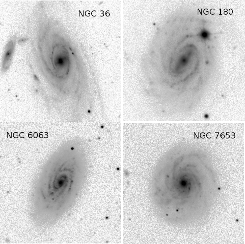
Figure 1: Images of the target galaxies are shown in the Sloan Digital Sky Survey (SDSS) $g$ filter ($4686\AA$). The images are taken from the NASA Extragalactic Database (NED). North is up and east is to the left.

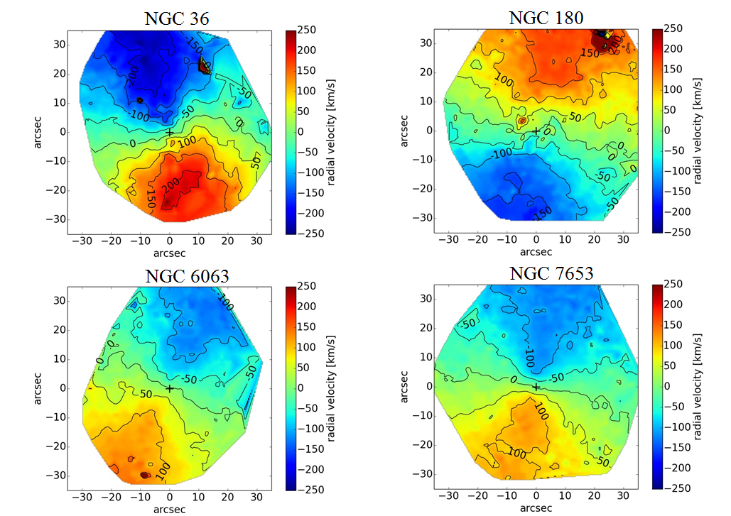
Figure 2: The colour-coded maps of the observed velocity fields in the target galaxies corrected for the systemic velocity of the respective galaxy as a whole. The lines show the contours of equal line-of-sight velocities. The contours are separated by $50$ km s^-1. The position of the centre of the galaxy is marked by a plus sign.

2 The Data

We selected four galaxies from the sample of CALIFA galaxies studied in Zinchenko et al. (2016). We chose galaxies where the spaxels with measured emission lines are homogeneously distributed over the image of the galaxy. Images of the target galaxies in the Sloan Digital Sky Survey (SDSS) $g$ filter are shown in Fig. 1. The images are taken from the NASA Extragalactic Database (NED). The processing of the observational data is reported in Zinchenko et al. (2016). Therefore we just briefly describe the data analysis steps and report additional measurements performed here.

We used publicly available spectra from the CALIFA survey data release 2 (DR2; Sánchez et al. (2012a); García-Benito et al. (2015); Walcher et al. (2014)), based on observations with the PMAS/PPAK integral field spectrophotometer mounted on the Calar Alto 3.5-m telescope in Spain. We used the low-resolution data cubes (setup V500) to determine the spatial distribution of the physical parameters of the interstellar ionized gas. The integrated stellar spectra in all spaxels were fitted using the public version of the STARLIGHT code (Cid Fernandes et al., 2005; Mateus et al., 2006; Asari et al., 2007) adapted for execution in the NorduGrid ARC environment of the Ukrainian National Grid. We used a set of 45 synthetic simple stellar population (SSP) spectra with metallicities $Z=0.004$, 0.02, and 0.05, and 15 ages from 1 Myr up to 13 Gyr from the evolutionary synthesis models of Bruzual & Charlot (2003), and the reddening law of Cardelli et al. (1989) with $R_{V}=3.1$. The nebular emission spectrum in each spaxel was obtained by subtracting the stellar population synthesis spectrum from the observed one. The profiles of H$\beta$, H$\alpha$, [OIII]$\lambda\lambda$4959,5007, [NII]$\lambda\lambda$6548,6584, and [SII]$\lambda\lambda$6717,6731 lines were fitted by Gaussians.

The line-of-sight velocity of the interstellar gas was determined from the wavelength of the centre of the H$\alpha$ line profile. The observed velocity fields of the target galaxies corrected for the systemic velocity of each galaxy, $V_{sys}$, are shown in Fig. 2. We list the inferred values of $V_{sys}$ in Table 3.

The measured line fluxes were corrected for interstellar reddening using the theoretical H$\alpha$ to H$\beta$ ratio from Osterbrock (1989), assuming case B recombination, an electron temperature of 10,000 K, and the analytical approximation to the Whitford interstellar reddening law by Izotov et al. (1994). If the measured value of the ratio H$\alpha$/H$\beta$ is lower than the theoretical one (2.86) then the reddening is adopted to be zero.

We used the oxygen abundances determined in Zinchenko et al. (2016) through a strong-line method (the $C$ method, Pilyugin et al., 2012). It should be noted that the $C$ method produces oxygen abundances compatible to the metallicity scale defined by H ii regions with $T_{e}$-based abundances.

For the further analysis of the velocity field and the extinction map we selected spaxels with a ratio of the flux to the flux error $\epsilon\geq 8$ for the H$\alpha$ emission line. For the oxygen abundance map, only spaxels with $\epsilon\geq 3$ for the each of the H$\beta$, H$\alpha$, [OIII]$\lambda$5007, [NII]$\lambda$6584 lines were selected for further analysis.

The properties of our target galaxies are given in Table 1. The galaxy name is reported in the first column. The morphological type and the morphological type code $T$ of the galaxy taken from the LEDA data base (Paturel et al., 2003) are reported in Columns 2 and 3. The stellar mass of the galaxy and its absolute magnitude are listed in Columns 4 and 5. The galaxy inclination and position angle of the major axis obtained from the analysis of the photometric map are reported in Columns 6 and 7. The isophotal radii $R_{25}$ in arcmin and in kpc are given in Columns 8 and 9, respectively. The adopted distance is listed in Column 10.

Our subsequent study is based on the maps of velocity, oxygen abundance, and extinction $A_{V}$ (Balmer decrement) of the four galaxies.

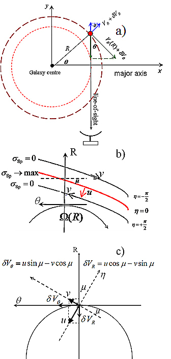
Figure 3: $a)$ Contributions of the different components of the gas motion to the line-of-sight velocity. $b)$ The velocity field of a spiral density wave. $\sigma_{Sp}$ denotes the density perturbation of the galactic disc. The pitch angle of the spiral arm, $\mu$, is defined as the angle between tangents to the circle and to the spiral arm. The lines of equal spiral arm phase, $\eta=const$, are lines of equal density and velocity perturbation. The component of the streaming velocity perpendicular to the spiral arm, $u$, has its extreme value at $\eta=0$. The tangential streaming velocity, $v$, reaches its extreme values for $\eta=\pm\pi/2$, i.e., at the outer and inner spiral arm borders (perturbed density $\sigma_{Sp}=0$). $c)$ The radial (along the direction of increasing galactocentric distance) and tangential (parallel to the direction of rotation) components of the velocity perturbations ($\delta V_{R}$, $\delta V_{\theta}$) are related to the streaming velocity $(u,v)$ by Eq. 5 and depend on the pitch angle $\mu$.

3 The kinematic spiral arms

3.1 Fourier coefficients from the velocity field

The Fourier transformation method is used to decompose a two-dimensional velocity field into a hierarchy of structures on different scales. This method, applied to a number of narrow concentric annuli in radial direction of the galaxy, allows one to extract the field of perturbations in both the angular and radial components of the velocity and to investigate logarithmic and other types of spiral arms. It should be noted that there is no assumption of the shape of the spiral arms with this method. In the current Section this method is applied to the two-dimensional velocity fields to investigate the spiral structure of the velocity perturbations arising due to spiral density waves.

The line-of-sight velocity field of the gas in galactic discs exhibits deviations from a purely circular motion, which are associated with the spiral arms of the galaxy (Visser, 1980). These deviations could be due to the influence of a spiral density wave on the circular rotation of the gas in the disc (Lin et al., 1969). The tangential and radial components of perturbed velocities ($\delta V_{\theta}$, $\delta V_{R}$) caused by a spiral density wave depend on the amplitude of the wave, the position of the corotation and Lindblad resonances, and the mass distribution within the galaxy. Here $R$ is the deprojected galactocentric distance in the plane of the galaxy and $\theta$ is the polar angle, measured from the major axis of the galaxy. There can also be deviations from pure circular motions of other types, e.g., a radially symmetric outflow or inflow toward the center of the galaxy, caused by bars, warps, lopsidedness, or a galactic fountain (e.g., Bosma, 1978; Sakhibov & Smirnov, 1987, 1989, 1990, 2004; Fraternali et al., 2001; Schinnerer et al., 2000). The description of different approaches to the modelling of non-circular motions in a two-dimensional velocity map is given in Spekkens & Sellwood (2007), where the non-circular motions with rather high velocities due to a bar-like distortion of an axisymmetric potential are considered. The objective of the present paper is to examine the non-circular motions caused by density wave perturbations. It is expected that the radial velocities caused by a bar can exceed the non-circular velocities caused by density wave perturbations in the bar region. We will investigate the non-circular motions in the disc outside the bars where radial velocities caused by the spiral perturbation are expected to make a dominant contribution to the non-circular motions.

The contributions of the perturbed tangential ($\delta V_{\theta}$) and radial ($\delta V_{R}$) components of the velocity to the observed line-of-sight velocity are given by the equation (see Fig. 3a)

$$V_{sp}=\Bigl{(}\delta V_{\theta}(R,\theta)\cdot\cos\theta+\delta V_{R}(R,\theta)\cdot\sin\theta\Bigl{)}\cdot\sin i$$ (1)

Thus, the line-of-sight velocity $V^{obs}_{r}(R,\theta)$ observed at a given point of the disc involves the velocity of the galaxy as a whole, $V_{gal}$, the rotation velocity, $V_{\theta}(R)$, a pure radial inflow or outflow $V_{R}$, and the velocities $\delta V_{\theta}$ and $\delta V_{R}$ caused by the density wave perturbation (see Fig. 3a).

$$\frac{V^{obs}_{r}(R,\theta)}{\sin i}=V_{gal}+\Bigl{(}V_{\theta}(R)+\delta V_{\theta}(R,\theta)\Bigl{)}\cdot\cos\theta+\Bigl{(}V_{R}+\delta V_{R}(R,\theta)\Bigl{)}\cdot\sin\theta$$ (2)

where $i$ is the inclination angle of the galaxy.

Our aim is to extract the contributions caused by the spiral density wave, $\delta V_{\theta}$ and $\delta V_{R}$, to the observed velocity $V^{obs}_{r}(R,\theta)$. If the gravitational potential of a disc galaxy is perturbed by a rotating spiral wave, the gas in the disc reacts by streaming motions that are also of spiral shape. The response of the gas then is

$$u=\hat{u}\cos\eta$$ (3)

$$v=-\hat{v}\sin\eta$$

where $\eta$ is the phase of the perturbation by a spiral wave (which varies across the spiral arm, see Fig. 3b)

$$\eta=-m\theta+mh\cot\mu\ln{(R/R_{0})}$$ (4)

where $h=+1$ and $h=-1$ for an S- and Z-spiral arm, respectively, $\mu$ is the pitch angle (a measurement of the tightness of the winding of spiral arms), and $m$ is the number of the arms. The parameter h determines the direction of winding of the spiral arm in the sky: S-shaped or Z-shaped. Note that a right-handed coordinate system is used. The values $\hat{u}$ and $\hat{v}$ are amplitudes (extreme values) of orthogonal (across the spiral arm) and tangential streaming velocities. The orthogonal streaming velocity has its extreme value at the centre of the spiral arm for $\eta=0$ and the tangential streaming velocity has its extreme values at the outer and inner spiral arm borders for $\eta=\pm\pi/2$ (Fig. 3b).

The orthogonal and tangential streaming velocities make a contribution to the observed line-of-sight velocity $V^{obs}_{r}(R,\theta)$ in the form of the velocity perturbations ($\delta V_{R}$, $\delta V_{\theta}$). The radial (along the direction of increasing galactocentric distance) and tangential (parallel to the direction of rotation) components of the velocity perturbations ($\delta V_{R}$, $\delta V_{\theta}$) are related to the streaming velocity $(u,v)$ by Eq. 5 and depend on the geometrical form (pitch angle $\mu$) of the spiral arm (see Fig. 3c)

$$\delta V_{\theta}=h(u\sin\mu-v\cos\mu)$$ (5)

$$\delta V_{R}=u\cos\mu-v\sin\mu$$

Using Eq. (3) to Eq. (5) and grouping the sine and cosine terms of identical quantities of $\theta$, the perturbed motion $V_{sp}$ (Eq. (1)) caused by the mode $m$ can be written in the form

$$V_{sp}=\frac{1}{2}(\hat{u}-\hat{v})\cdot\cos\Bigl{(}(m-1)\theta\Bigr{)}\cdot\sin\Bigl{(}m\cot\mu\ln{(R/R_{0})+\mu\Bigr{)}}$$

$$-\frac{1}{2}(\hat{u}-\hat{v})\cdot\sin\Bigl{(}(m-1)\theta\Bigr{)}\cdot\cos\Bigl{(}m\cot\mu\ln{(R/R_{0})+\mu\Bigr{)}}$$ (6)

$$-\frac{1}{2}(\hat{u}+\hat{v})\cdot\cos\Bigl{(}(m+1)\theta\Bigr{)}\cdot\sin\Bigl{(}m\cot\mu\ln{(R/R_{0})-\mu\Bigr{)}}$$

$$+\frac{1}{2}(\hat{u}+\hat{v})\cdot\sin\Bigl{(}(m+1)\theta\Bigr{)}\cdot\cos\Bigl{(}m\cot\mu\ln{(R/R_{0})-\mu\Bigr{)}}$$

Eq. (3.1) corresponds the case of $h=+1$, because all our target galaxies are S-spirals. The coefficients of the sines and cosines of the polar angles $(m-1)\theta$ and $(m+1)\theta$ determine the contribution of the velocity perturbations to the observed line-of-sight velocity. Inspection of Eq. (3.1) shows that the second mode of the spiral-density wave ($m=2$) – a two-armed spiral – contributes to the values multiplied by the sines and cosines of the polar angles $\theta$ and $3\theta$ while the first mode ($m=1$) – a one-armed spiral – contributes to the values multiplied by the sines and cosines of the polar angles $\theta=0$ and $2\theta$.

Eq. (3.1) and Eq. (2) result in

$$\frac{V^{obs}_{r}(R,\theta)}{\sin i}=a_{0}+a_{1}\cos(\theta)+b_{1}\sin(\theta)+$$

$$+a_{2}\cos(2\theta)+b_{2}\sin(2\theta)+a_{3}\cos(3\theta)+b_{3}\sin(3\theta)$$ (7)

where the coefficients $a_{0},a_{1},b_{1},a_{2},b_{2},a_{3}$, and $b_{3}$ are

$$a_{0}=V_{gal}+\frac{1}{2}(\hat{u}_{1}-\hat{v}_{1})\cdot\sin\Bigl{(}\cot\mu_{1}\ln{(R/R_{01})+\mu_{1}\Bigr{)}}$$

$$a_{1}=V_{\theta}(R)+\frac{1}{2}(\hat{u}_{2}-\hat{v}_{2})\cdot\sin\Bigl{(}2\cot\mu_{2}\ln{(R/R_{02})+\mu_{2}\Bigr{)}}$$

$$b_{1}=V_{R}-\frac{1}{2}(\hat{u}_{2}-\hat{v}_{2})\cdot\cos\Bigl{(}2\cot\mu_{2}\ln{(R/R_{02})+\mu_{2}\Bigr{)}}$$ (8)

$$a_{2}=-\frac{1}{2}(\hat{u}_{1}+\hat{v}_{1})\cdot\sin\Bigl{(}\cot\mu_{1}\ln{(R/R_{01})-\mu_{1}\Bigr{)}}$$

$$b_{2}=\frac{1}{2}(\hat{u}_{1}+\hat{v}_{1})\cdot\cos\Bigl{(}\cot\mu_{1}\ln{(R/R_{01})-\mu_{1}\Bigr{)}}$$

$$a_{3}=-\frac{1}{2}(\hat{u}_{2}+\hat{v}_{2})\cdot\sin\Bigl{(}2\cot\mu_{2}\ln{(R/R_{02})-\mu_{2}\Bigr{)}}$$

$$b_{3}=\frac{1}{2}(\hat{u}_{2}+\hat{v}_{2})\cdot\cos\Bigl{(}2\cot\mu_{2}\ln{(R/R_{02})-\mu_{2}\Bigr{)}}$$

Hereafter the quantities $\hat{u}_{1}$, $\hat{v}_{1}$, $\mu_{1}$, and $R_{01}$ mean the velocity perturbation amplitudes, the pitch angle, and scaling factor for the first mode ($m=1$), and $\hat{u}_{2}$, $\hat{v}_{2}$, $\mu_{2}$, and $R_{02}$ stand for the velocity perturbation amplitudes, the pitch angle, and the scaling factor for the second mode ($m=2$) of a spiral density wave, respectively.

The systemic velocity $V_{gal}$ of the galaxy (not corrected for inclination) contributes in the zeroth Fourier harmonic and mixes with the velocity perturbation from the first mode $m=1$ of the spiral density wave.

The circular rotation $V_{\theta}(R)$ contributes in the first Fourier harmonics ($a_{1}$) and mixes with the velocity perturbation from the second mode $m=2$ of the spiral density wave.

The first mode of the spiral wave ($m=1$) – a one-armed asymmetric structure – contributes to the zeroth and second Fourier harmonics of the azimuthal distribution of the observed line-of-sight velocities. The second mode of the spiral-density wave ($m=2$) – a two-armed spiral – contributes also to the first and third Fourier harmonics of the azimuthal distribution of line-of-sight velocities at a given galactocentric distance, $R$. Since the zeroth Fourier coefficient, $a_{0}$, may include a contribution not only from the systemic velocity of the galaxy $V_{gal}$ but also from the first mode of the spiral density wave, the zeroth Fourier coefficient must change in radial direction along the galactic disc.

Thus, if the velocity of the galaxy, $V_{gal}$, and the radial change of the Fourier coefficients, $a_{1}(R)$, are determined, the pure rotation curve of the galaxy, $V_{\theta}(R)$, can be measured. The radial variation of the coefficients $a_{2}(R),b_{2}(R),a_{3}(R)$, and $b_{3}(R)$ defines the amplitude of the velocity perturbations caused by the spiral arms as well as the geometric form of the arms. Thus, the problem of the analysis of the residual velocities caused by a spiral density wave can be reduced to the determination of the first three harmonics of the Fourier series of the observed azimuthal distribution of the line-of-sight velocities for the thin ring zones.

There is also an impact of the bar in the inner part of a barred galaxy. Accounting for the impact of the bar, according to the bisymmetric model by Spekkens & Sellwood (2007), changes Eq. 2 for the observed line-of-sight velocity:

$$\frac{V^{obs}_{r}(R,\theta)}{\sin i}=V_{gal}+\Bigl{(}V_{\theta}(R)+\delta V_{\theta}(R,\theta)+V_{2,t}\Bigl{)}\cdot\cos\theta+$$

$$+\Bigl{(}V_{R}+\delta V_{R}(R,\theta)+V_{2,r}\Bigl{)}\cdot\sin\theta$$ (9)

where $V_{2,t}=\hat{V}_{2,t}\cos(2\theta_{b})$ and $V_{2,r}=\hat{V}_{2,r}\sin(2\theta_{b})$ are the tangential and radial components of the non-circular flow caused by the bar. These components vary with the angle to the bar axis $\theta_{b}=\theta-\phi_{b}$ as the cosine and sine of $2\theta_{b}$, respectively. The major axis of the bar lies at an angle $\phi_{b}$ to the projected major axis of the galaxy (see Fig. 1 in Spekkens & Sellwood (2007)). The maximal amplitudes of the tangential and radial components of the non-circular flow caused by bar, $\hat{V}_{2,t}(R)$ and $\hat{V}_{2,r(R)}$, respectively, are both functions of the radius. Eq. 3.1 can be rewritten as:

$$a_{0}=V_{gal}+\frac{1}{2}(\hat{u}_{1}-\hat{v}_{1})\cdot\sin\Bigl{(}\cot\mu_{1}\ln{(R/R_{01})+\mu_{1}\Bigr{)}}$$

$$a_{1}=V_{\theta}(R)+\frac{1}{2}(\hat{u}_{2}-\hat{v}_{2})\cdot\sin\Bigl{(}2\theta_{Sp2}+\mu_{2}\Bigr{)}-\frac{1}{2}(\hat{V}_{2,t}-\hat{V}_{2,r})\cdot\sin\Bigl{(}2\phi_{b}\Bigr{)}$$

$$b_{1}=V_{R}-\frac{1}{2}(\hat{u}_{2}-\hat{v}_{2})\cdot\cos\Bigl{(}2\theta_{Sp2}+\mu_{2}\Bigr{)}+\frac{1}{2}(\hat{V}_{2,t}-\hat{V}_{2,r})\cdot\cos\Bigl{(}2\phi_{b}\Bigr{)}$$ (10)

$$a_{2}=-\frac{1}{2}(\hat{u}_{1}+\hat{v}_{1})\cdot\sin\Bigl{(}\cot\mu_{1}\ln{(R/R_{01})-\mu_{1}\Bigr{)}}$$

$$b_{2}=\frac{1}{2}(\hat{u}_{1}+\hat{v}_{1})\cdot\cos\Bigl{(}\cot\mu_{1}\ln{(R/R_{01})-\mu_{1}\Bigr{)}}$$

$$a_{3}=-\frac{1}{2}(\hat{u}_{2}+\hat{v}_{2})\cdot\sin\Bigl{(}2\theta_{Sp2}-\mu_{2}\Bigr{)}-\frac{1}{2}(\hat{V}_{2,t}+\hat{V}_{2,r})\cdot\sin\Bigl{(}2\phi_{b}\Bigr{)}$$

$$b_{3}=\frac{1}{2}(\hat{u}_{2}+\hat{v}_{2})\cdot\cos\Bigl{(}2\theta_{Sp2}-\mu_{2}\Bigr{)}+\frac{1}{2}(\hat{V}_{2,t}+\hat{V}_{2,r})\cdot\cos\Bigl{(}2\phi_{b}\Bigr{)}$$

where $\theta_{Sp2}=\cot\mu_{2}\ln{(R/R_{02})}$ belongs to the bisymmetrical (mode $m=2$) of the spiral perturbations. Eq. 3.1 shows that the spiral term at the coefficients $a_{1},b_{1},a_{3},b_{3}$ is modulated by the periodic sine or cosine functions. The amplitudes of the tangential and radial components of the non-circular flow caused by the bar, $\hat{V}_{2,t}(R)$ and $\hat{V}_{2,r(R)}$, respectively, are both functions of the radius. Since the elliptical bar potential decreases monotonously with radius $R$ the bar term in Eq. 3.1 also decreases monotonously. Eq. 2 and Eq. 3.1 correspond to the radial model by Spekkens & Sellwood (2007) with additional terms of spiral perturbations. Eq. 3.1 and Eq. 3.1 correspond to the bisymmetric model by the same authors with additional terms of spiral perturbations. We refer to the model described by Eq. 2 and Eq. 3.1 as the radial model with spiral perturbations and to the model described by Eq. 3.1 and Eq. 3.1 as the bisymmetric model with spiral perturbations.

In the outer part of the galaxy, the impact of the elliptical bar potential decreases quickly with radius $R$. A bar term would add to the radial symmetric (outflow/inflow) motion and the impact of the spiral term, or vanish. This means that beyond the bar Eq. 3.1 and Eq. 3.1 will coincide with Eq. 2 and Eq. 3.1. Since our main goal is a study of the impact of spirals on the spatial distribution of tracers, we adopt the radial model with spiral perturbations (Eq. 2 and Eq. 3.1) outside the bar. The pure radial outflow or inflow velocities contribute to the first Fourier harmonic ($b_{1}$) while the pitch angle $\mu_{2}$ and characteristic radius $R_{02}$ will be determined from the third Fourier harmonic. The radial disturbance by the bar has no impact on the definition of the geometrical parameters of the spiral arms.

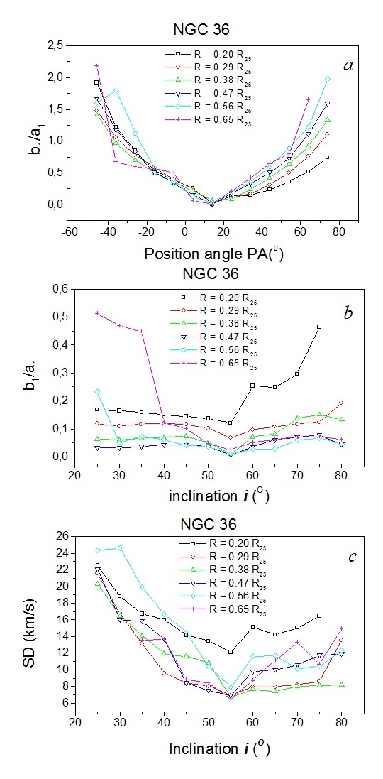
Figure 4: The change of the ratio of the Fourier coefficients $b_{1}/a_{1}$ in dependence on the proposed values of position angle $PA$ (a) and inclination angle $i$ (b) in NGC 36. c)The change of the standard deviation $SD$ of the observed line-of-sight velocities from the predicted ones in dependence on the proposed values of the inclination angle $i$ in NGC 36.

3.2 Determination of the galaxy inclination and the position angle of the major axis

Here we estimate the galaxy inclination and the position angle of the major axis from the analysis of the observed velocity field and compare them with the values for the same quantities obtained from the analysis of the surface brightness distribution (Zinchenko et al., 2016). One may expect that the rotation makes a dominant contribution to the observed line-of-sight velocities. This means that the ratio of the Fourier coefficients $b_{1}/a_{1}$ is minimized if the galaxy inclination and position angle of the major axis are correct. It is expected that the velocities of the radially symmetric motions $V_{R}$ are within 10 – 20 km s^-1, the velocities of the spiral perturbations $\delta V_{R}$ within 5 – 10 km s^-1 (Rohlfs, 1977), and the rotation velocities $V_{\theta}$ within 150 – 300 km s^-1. Then the expected value of the ratio $b_{1}/a_{1}$ does not exceed $10\%-15\%$ if the values of $i$ and $PA$ are correct. The radial velocities can reach unrealistically large values (which may be comparable to the rotation velocities or even exceed them) if the values of $i$ and $PA$ are not correct. Thus, $PA$ and $i$ are estimated from the requirement that the ratio of the Fourier coefficients $b_{1}/a_{1}$ is minimized for the correct values of $i$ and $PA$.

We first consider a set of values of galaxy inclinations and position angles of the major axis with large steps, $\Delta i=5\degr$ and $\Delta P=10\degr$. A set of deprojected coordinates of individual pixels in the target galaxy for each set of the values of $i$ and $PA$ is obtained. Then a set of the coefficients $a_{0},a_{1},b_{1},a_{2},b_{2},a_{3},$ and $b_{3}$ of Eq. (3.1) is determined for each set of the deprojected coordinates of the individual pixels by fitting to the line-of-sight velocities. The disc is divided into annuli of width $\Delta R$ = 1 kpc in the plane of the target galaxy (see 3.5). The coefficients $a_{0},a_{1},b_{1},a_{2},b_{2},a_{3},$ and $b_{3}$ are assumed to be equal for all the pixels within a given annulus. Assuming that the rotation makes a dominant contribution to the observed line-of-sight velocities we choose the values of $i$ and $PA$ that minimize the ratio of the Fourier coefficients $b_{1}/a_{1}$ as an approximation of the position angle of the major axis and the inclination angle of the galaxy. Fig. 4(a,b) shows the Fourier coefficient ratio $b_{1}/a_{1}$ as a function of $PA$ and $i$ for the galaxy NGC 36. To avoid crowding in the diagrams, the data are presented for the interval from 4.5 kpc to 14.5 kpc (from $0.20R_{25}$ to $0..65R_{25}$) with a step size of 2 kpc. Each curve corresponds to a single annulus. The step size in $PA$ is $\Delta_{PA}=10\degr$ and the step size in $i$ is $\Delta_{i}=5\degr$. Each ring zone shows a different $b_{1}/a_{1}$ value, but every curve has its minimum at the same $PA=14\degr$ and at the same $i=55\degr$. In some zones the minimum of the curve in the $b_{1}/a_{1}$ vs. $i$ diagram is not so prominent as in the $b_{1}/a_{1}$ vs. $PA$ diagram. Therefore, we consider an additional diagram. Fig. 4(c) shows the standard deviation SD of the observed line-of-sight velocity in an annulus compared to the one predicted by Eq. 3.1 as a function of inclination angle $i$ for NGC 36. The minimum value of the SD occurs at the same inclination $i=55\degr$ as in the previous $b_{1}/a_{1}$ vs. $i$ diagram. Every annulus shows different SD values, but almost all curves have a similar minimum of SD $\approx$ (6–8) km s^-1 at the same $i=55\degr$.

Next, we use a set of $PA$ and $i$ values with smaller step sizes of $2\degr$ to find more accurate values of the $PA$ and $i$ for the target galaxies. The obtained values of $PA$ and $i$ are listed in Table 3 (Columns 2 and 3, respectively) and are used below to find the deprojected coordinates of the spaxels with measured oxygen abundance and Balmer decrement.

Our obtained values of $PA$ and $i$ are generally in agreement with the photometry-based values of the $PA$ and $i$ reported in Table 1. The inclination of the galaxy NGC 36 determined here from the kinematics ($i=55\degr$) agrees with axis ratio $b/a=0.56$ reported in the Uppsala General Catalogue of Galaxies (Nilson, 1973) and is close to the $b/a=0.62$ given in the Third Reference Catalogue of Bright Galaxies (RC3 de Vaucouleurs et al, 1991)

We only find a significant discrepancy between the values of the $PA$ determined by the different methods for the galaxy NGC 7653: $PA=140\degr$ listed in the NED data base based on the angular diameters measured in $K_{s}$ (2MASS “total”) passband, $PA=172.5\degr$ given in the LEDA data base, $PA=175\degr$ based on the photometry map of Zinchenko et al. (2016), and $PA=165\degr$ obtained here for the velocity map. It should be noted that NGC 7653 is a nearly face-on galaxy.

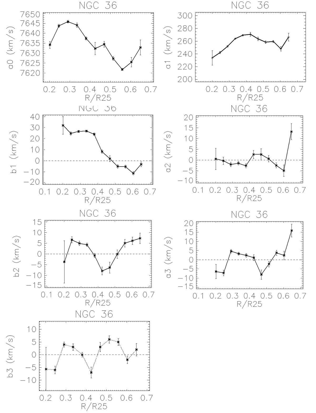
Figure 5: The radial change of the Fourier coefficients $a_{0}$, $a_{1}$, $b_{1}$, $b_{2}$, $a_{3}$, and $b_{3}$ in NGC 36.

3.3 Determination of the systemic velocity of galaxies from the velocity map

The deprojected coordinates of each pixel in the target galaxy are determined with the position angle of the major axis and the galaxy inclination obtained in Subsection 3.2. The galactic disc is divided into several annuli of a width of $\Delta R=1$ kpc. For every annulus, we determine the seven unknown Fourier coefficients $a_{0},a_{1},b_{1},a_{2},b_{2},a_{3},$ and $b_{3}$ of Eq. (3.1) using a least-squares method. The step size of $\Delta R=1$ kpc provides 50 to 200 data points in each annulus in the interval of galactocentric distances from $R\sim 0.2R_{25}$ to $R\sim R=0.7R_{25}$. Thus the number of data points (spaxels) in each annulus is large enough for a reliable determination of the coefficients of Eq. (3.1). The determinations of the coefficients $a_{0},a_{1},b_{1},a_{2},b_{2},a_{3},$ and $b_{3}$ in a several annuli allows us to assess the radial change of these coefficients.

Fig. 5 shows an example of the radial change of the coefficients $a_{0},a_{1},b_{1},a_{2},b_{2},a_{3},$ and $b_{3}$ in case of NGC 36. The range of galactocentric distances where the coefficients were determined covers a large part of the disc from approximately $R=0.2R_{25}$ to $R=0.7R_{25}$. As was noted in Subsection 3.1 the Fourier coefficients contain information on the systemic velocity of the galaxy, $V_{gal}$, the pure circular motion, $V_{\theta}(R)$, the radially symmetric motion, $V_{R}$, the peculiar velocities caused by the spiral arms, and the geometric shape of the arms.

First we estimate the systemic velocity $V_{sys}$ of the galaxy, which is a projection of the velocity of the galaxy as a whole along the line-of-sight. As noted above (Section 3, Eq.(̃3.1)), the zeroth Fourier coefficient $a_{0}$ includes contributions from the first mode of the spiral density wave and from the space velocity of the galaxy.

If the true value of the systemic velocity $V_{sys}$ is subtracted from the line-of-sight velocity of each point (spaxel) then the coefficient $a_{0}$ expresses the impact of the spiral wave only and changes along the radius as a sine function

$$a_{0}=\frac{1}{2}\Bigl{(}\hat{u}_{1}-\hat{v}_{1}\Bigr{)}\cdot\sin\Bigl{(}\cot\mu_{1}\ln{(R/R_{01})+\mu_{1}\Bigr{)}}.$$ (11)

The radially averaged value of $a_{0}$ must be close to zero, and the absolute value of maximum positive and negative amplitudes must be equal to each other. This condition can be used to estimate the true value of the systemic velocity $V_{sys}$. To do so, we constructed a set of diagrams of $a_{0}$ vs. $R$ for different values of the $V_{sys}$. The value of the $V_{sys}$ for which the absolute values of the maximum positive and negative values of the $a_{0}$ are equal to each other is adopted to be true. In this case, the absolute value of the $a_{0}$ corresponds to the amplitude of the non-circular perturbations caused by the spiral density wave.

Fig. 6 shows the value of $a_{0}$ obtained with the true $V_{sys}$ as a function of galactocentric distance for each galaxy. We assume that Fig. 6 shows the radial change of the non-circular perturbation caused by the first mode ($m=1$) of the spiral density wave in our target galaxies. The bars in Fig. 6 show the errors of the zeroth Fourier coefficients $a_{0}$, determined from the standard least-squares procedure. The large number (50 – 200) of the conditional equations (because of the large number of measurements) in each annulus provides low uncertainties of $a_{0}$, i.e., the errors are significantly lower than the amplitude of the non-circular perturbations caused by the spiral density wave. One can see from Fig. 6 that the amplitude of non-circular velocities is around 10 km s^-1, which agrees with the line-of-sight components of the density wave motions predicted by the model (see Fig. 12 in Rots (1975)). This fact can be considered as additional evidence in favor of the validity of the value of $V_{sys}$.

Our estimates of the systemic line-of-sight velocities $V_{sys}$ agree with the values of other authors (listed in the NED database): $6224\pm 12$ km s^-1 for NGC 36 (Karachentsev & Makarov, 1996), $5394\pm 5$ km s^-1 for NGC 180 (de Vaucouleurs et al, 1991), $2944\pm 8$ km s^-1 for NGC 6063 (Fixsen et al., 1996), and $4378\pm 20$ km s^-1 for NGC 7653 (Mould et al., 2000).

The obtained values of the systemic velocities of the target galaxies are given in Column 4 of Table 3. The uncertainty of the systemic velocity $V_{sys}$ is estimated as the sum of the error in the line-of-sight velocity and the maximum amplitude of the first mode.

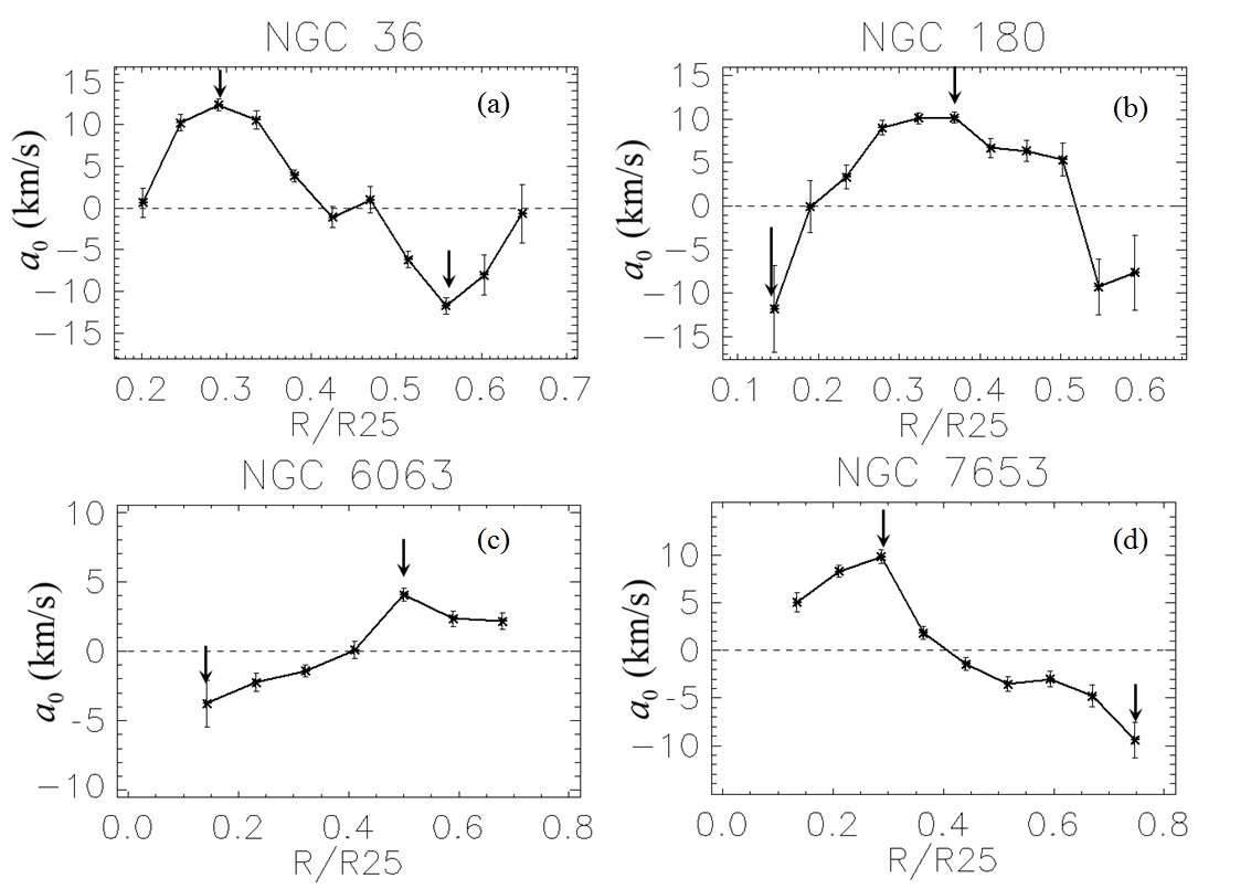
Figure 6: The coefficient $a_{0}$, computed for the true $V_{sys}$, as a function of galactocentric distance in our target galaxies. The $a_{0}(R)$ illustrates the radial change of the non-circular perturbations of the velocity caused by the first mode ($m=1$) of the spiral density wave (see Eq. 11). The arrows show the positions of the maximum positive and negative amplitudes of perturbations, caused by the spiral density wave.

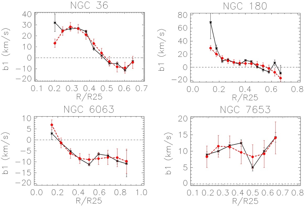
Figure 7: Fourier coefficient $b_{1}$ as a function of galactocentric distance in our target galaxies (black curve). The Fourier coefficient $b_{1}$ illustrates the radial change of non-circular perturbations of the velocity caused by the radially symmetric motion $V_{R}$ and the second mode ($m=2$) of the spiral density wave (see Eq. 3.1). The red curve is a model used to determine the radially symmetric motion $V_{R}$ and the amplitude of the velocity perturbation caused by the second mode of the spiral density wave.

3.4 Radially symmetric motions in the target galaxies obtained from velocity maps

The radially symmetric motion $V_{R}$ can be determined from the radial change of the first Fourier harmonics (black curves in Fig. 7). Expression 3 of Eq. 3.1 shows that the radial motion $V_{R}$ contributes to the Fourier coefficient ($b_{1}$) and mixes with the velocity perturbation from the second mode $m=2$ of the spiral density wave. First, we consider the barred galaxies NGC 36 and NGC 180. There are large radial velocities of $V_{R}>30$ km s^-1 (NGC 36) and $V_{R}>60$ km s^-1 (NGC 160) in the inner parts of both barred galaxies. We assume that this is an effect of the bar. The large error of coefficient $b_{1}$ in these points suggests that there is an explicit contribution of radial streaming velocities of the bar to the azimuthally averaged radial motion in NGC 36 and NGC 180.

Fig. 7 shows that there is a periodical component of the radial motion in the middle and outer parts of disc. The periodical component of the coefficient $b_{1}$ is shifted relative to the zero velocity line (dashed line in Fig. 7). This may be an effect of the large-scale radial outflow/inflow motion outside of the bar region. We approximated the radial change of the coefficient $b_{1}$ by a polynomial function of the third degree (red curve). As a sine or cosine shape of the variable term of the polynomial in barred galaxies corresponds rather to the spiral term than the bar term in Eq. 3.1, we made the simplest assumption that the variable term of the polynomial describes the impact of the spirals. The constant term may be explained as an azimuthally averaged radial outflow/inflow motion, while the impact of the bar term in the outer regions is negligible. This means that the coefficient $b_{1}(R)$ comprises generally the radial outflow/inflow motion $V_{R}$ and the radial component of the velocity perturbations from spirals. The relative small errors of the coefficient $b_{1}$ in the outer regions of the barred galaxies NGC 36 and NGC 180 may indicate that a contribution of radial streaming velocities in the bar to the azimuthally averaged radially symmetric motion in NGC 36 and NGC 180 is small outside the bar. So we explain the radial change of the coefficient $b_{1}(R)$ with the help of the radial model with spiral perturbations (Eq. 3.1). The curve can be interpreted as follows. The Fourier coefficient $b_{1}$ comprises a constant radially symmetric large-scale component $V_{R}$ and a periodical component of the non-circular motion caused by spiral perturbations outside the region with bar impact. Table 2 lists the radial velocities in our target galaxies. Similar radial velocities were detected in NGC 2976 by Spekkens & Sellwood (2007).

Table 2: Radially symmetric motion in our target galaxies.

Galaxy	$V_{R}$ (km/s)a
NGC 36	$9.1\pm 3.1$
NGC 180	$7.0\pm 3.4$
NGC 6063	$-4.6\pm 1.2$
NGC 7653	$10.1\pm 1.4$

^a Since the side of the disk nearest to the observer disk along the minor axis is unknown, it is not possible to distinguish between inflow and outflow motion.

3.5 Determination of the geometrical parameters of spiral arms from the velocity map

Despite the observational fact that spiral arms in a real galaxy never have a strict geometric form because other local structures may muddle their appearance, investigators always try to describe the large-scale spiral structure of galaxies using a model of regular geometric form. To minimize the influence of local structures, a large radial interval should be analyzed. On the other hand, observations show that the pitch angle can vary along the radius (the change can exceed $20\%$ (Savchenko & Reshetnikov, 2013)). This suggests that a small radial interval should be analysed. Therefore the number of annuli used to determine the pitch angle is smaller than the total number of annuli adopted when the Fourier coefficients were computed.

Figure 8: The radial change of the Fourier coefficients $a_{3}$ and $b_{3}$ in NGC 180 shows that starting at about $0.2R_{25}$, the periodic component associated with the spiral velocity perturbation dominates the monotonically decreasing component of the bar term in the coefficients $a_{3}$ and $b_{3}$ from equation Eq. 3.1.

In the current study, we adopt a logarithmic form of spiral arms because it appears suitable and leads to a satisfactory fit. We should note that the procedure of the determination of the Fourier coefficients does not assume that the spiral arms are logarithmic. In earlier work, spirals of different shapes were compared with observed spiral structures (Considere & Athanassoula, 1982, and references therein). It was found (Considere & Athanassoula, 1982) that the deviations of logarithmic and other shapes of spiral arms are smaller than the dispersion in the positions of H ii regions or other arm tracers.

A logarithmic spiral is defined by the expression

$$R=R_{0}e^{(\tan(\mu)\cdot\theta)}$$ (12)

where $R$ and $\theta$ are polar coordinates in the plane of the galaxy, and $\mu$ is a pitch angle of the spiral arm.

The change of the coefficient $a_{0}$, computed for the true $V_{sys}$, with galactocentric distance (see Fig. 6 and Eq. 11) provides a possibility to define graphically the pitch angle $\mu_{1}$ of the spiral arm. The phase difference between the maximum positive and the maximum negative deviations from the (dashed) line of zero velocity is equal to $\pi$. Fig. 6a shows that the maximum positive deviation takes place at a galactocentric distance $R_{max}/R_{25}=0.31$ and the maximum negative deviation occurs at a galactocentric distance $R_{min}/R_{25}=0.58$ (marked with arrows) for the galaxy NGC 36. This results in a pitch angle of

$$\mu_{1}=\arctan\Bigl{(}\frac{1}{\pi}\ln\Bigl{(}\frac{R_{min}/R_{25}}{R_{max}/R_{25}}\Bigr{)}\Bigr{)}\approx 11\degr$$

where $R/R_{25}$ is a fractional radius (the galactocentric distance normalized to the disc’s isophotal radius at 25 mag arcsec^-2). The graphical determination of the places with a given phase difference, e.g., $\pi$, for other galaxies is an ambiguous task. Assuming that the curve is a periodic function we determine the maximum positive and maximum negative deviations from the condition that the phase difference is equal to $\pi$ (marked with arrows in Fig. 6). We find a pitch angle $\mu_{1}\approx 17\degr$ for NGC 180, $\mu_{1}\approx 22\degr$ for NGC 6063, and $\mu_{1}\approx 16\degr$ for NGC 7653.

The geometrical parameters of two-armed spirals $\mu_{2}$ and $R_{02}$ can be found from the radial change of the Fourier coefficients $a_{3}(R)$ and $b_{3}(R)$ (see Eq. 3.1). The sixth and seventh expressions of Eq. 3.1 give

$$\frac{a_{3}}{\sqrt{a_{3}^{2}+b_{3}^{2}}}=\sin\big{(}2\cot\mu_{2}\ln{(R/R_{02})}-\mu_{2}\big{)}$$ (13)

Eq. (13) can be rewritten as a linear regression

$$y=A+Bx$$ (14)

with the notations

$$x=\ln(R)$$

$$y=\arcsin\Biggl{(}\frac{a_{3}}{\sqrt{a_{3}^{2}+b_{3}^{2}}}\Biggr{)}$$

$$A=\mu_{2}-2\cot(\mu_{2})\cdot\ln(R_{02})$$

$$B=2\cot(\mu_{2})$$

The estimation of the coefficients of the regression (14) provides the geometrical parameters of two-armed spirals, $\mu_{2}$ and $R_{02}$. Table 3 (Col. 6) shows estimations of the pitch angle of $\mu_{2}$ of the two-armed spirals $\mu_{2}$ in our sample using velocity field perturbations.

We note the following: NGC 36 has a relatively short bar, $R_{bar}\approx 0.14R_{25}$. We determine the pitch angle $\mu_{2}$ and characteristic radius $R_{02}$ from the coefficients $a_{3}$ and $b_{3}$ computed in the annuli outside the bar. So our radial model with spiral perturbations (Eq. 2 and Eq. 3.1) is applied.

NGC 180 has a relatively long bar, $R_{bar}\approx 0.3R_{25}$. The coefficients $a_{3}$ and $b_{3}$ used in the determination of the pitch angle $\mu_{2}$ and characteristic radius $R_{02}$ were computed for a number of annuli, some of which lie at the end of bar (from $0.23R_{25}$ to $0.3R_{25}$) while the others are located outside the bar (from $0.3R_{25}$ to $0.4R_{25}$). Fig. 8 shows that starting at about $0.2R_{25}$, the periodic term associated with the spiral velocity perturbation in the expressions (Eq. 3.1) for the coefficients $a_{3}$ and $b_{3}$ dominates over the monotonically decreasing term associated with the bar.

The application of the radial model (Eq. 2 and Eq. 3.1) to the non-barred galaxies NGC 6063 and NGC 7653 works well.

Since the pitch angle can vary along the radius (the change can exceed 20% (Savchenko & Reshetnikov, 2013)), a limited interval of galactocentric distances $R$ was used in the determination of the pitch angle. This reduces the number of annuli, which lowers the accuracy of the pitch angle estimation. The intervals of galactocentric distances $R$ used for each tracer are given in Columns 7, 9, and 11 of the Table 3. These intervals do not cover the whole disc.

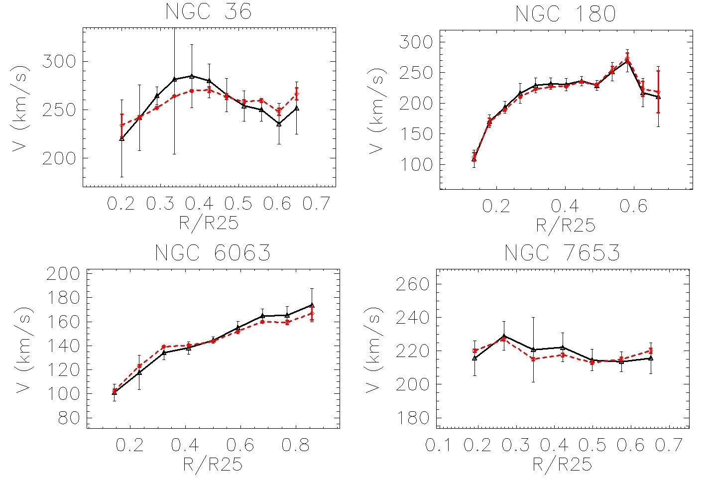
Figure 9: The rotation velocity $V_{\theta}(R)$ (solid black curve) and the value of the Fourier coefficient $a_{1}(R)$ (dotted red curve) as a function of galactocentric distance for the target galaxies.

Table 3: The derived properties of our target galaxies (the position angle of the major axis, $PA$, the galaxy inclination angle, $i$, the systemic velocity, $V_{gal}$, the maximum rotation velocity, $V_{max}$, the pitch angle of the spiral arms, $\mu_{2}$, and the scaling factor $R_{02}$).

Galaxy	$PA^{a}$	$i^{a}$	$V_{sys}$	$V_{max}$	$\mu_{2}^{b}$	$\Delta R^{b}$	$\mu_{2}^{c}$	$\Delta R^{c}$	$\mu_{2}^{d}$	$\Delta R^{d}$	$R_{02}$
	deg	deg	km/s	km/s	deg	$(R/R_{25})$	deg	$(R/R_{25})$	deg	$(R/R_{25})$	$(R/R_{25})$
1	2	3	4	5	6	7	8	9	10	11	12
NGC 36	14	55	6253$\pm$29	279	10	0.29 - 0.44	11	0.45 - 0.67	11	0.45 - 0.67	$0.53\pm 0.09$
NGC 180	165	46	5405$\pm$14	277	18	0.23 - 0.37	17	0.24 - 0.38	18	0.23 - 0.45	$0.29\pm 0.06$
NGC 6063	156	58	2945$\pm$11	168	23	0.34 - 0.48	24	0.54 - 0.85	22	0.36 - 0.63	$0.57\pm 0.15$
NGC 7653	165	31	4356$\pm$21	225	14	0.52 - 0.65	15	0.31 - 0.47	12	0.31 - 0.44	$0.43\pm 0.19$

$(^{a})$Uncertainties of the determination of $PA$ and $i$ are $\pm 2^{o}$.

$(^{b})$Value estimated from the velocity field.

$(^{c})$Value determined from the extinction map ratio $I_{H\alpha}/I_{H\beta}$.

$(^{d})$Value is obtained from the oxygen abundance map.

The step size intervals of the galactocentric distances $\Delta R$ used for the determination of the pitch angle of the spiral arms with different tracers are given in Columns 7, 9, and 11.

3.6 Rotation curves of the target galaxies obtained from velocity maps

The Fourier coefficients $a_{1}(R)$ and $b_{1}(R)$ of Eq. (3.1) can be used to determine the rotation curve of a galaxy. The second expression of Eq. (3.1) can be rewritten as

$$V_{\theta}(R)=a_{1}(R)-\frac{1}{2}(\hat{u}_{2}-\hat{v}_{2})\cdot\sin\big{(}2\cot\mu_{2}\ln{(R/R_{02})}-\mu_{2}\big{)}.$$ (15)

The spiral perturbations in Eq. 15 are accounted for using the pitch angle $\mu_{2}$ obtained in Sec. 3.5 and the amplitude derived from the Fourier coefficient $b_{1}$. Neglecting the tangential bar term in the Eq. 3.1 affects the estimation of the average rotation velocity and can result in a significant error of the rotation curve in the inner annuli for the galaxy NGC 180 with its long bar. The rotation curve of the galaxy NGC 36 with a small bar is derived outside the bar region.

Fig. 9 shows the rotation velocity $V_{\theta}(R)$ (solid black curve) and the value of the Fourier coefficient $a_{1}(R)$ (dashed red curve) as a function of galactocentric distance for the galaxies considered. We note that the error bar in the $a_{1}$ coefficient is substantially smaller than the error bar in $V_{\theta}$ except for a few cases, such as the last point of the rotation curve in NGC 180, where the large error of $a_{1}$ corresponds to the large error of $V_{\theta}$. Sources of large errors of rotation velocities $V_{\theta}(R)$ lie in the uncertainties of the pitch angle $\mu_{2}$ caused by the complex structure of the spiral patterns and variations of the pitch angle with galactocentric distance, as well as in uncertainties of the radial and tangential disturbances caused by the bar in barred galaxies. A precise determination of the pure rotation curve remains a difficult task and depends on the applied method of the decomposition of the observed velocities.

4 Spiral arms traced by abundance and extinction

Here we examine the manifestation of spiral arms in the oxygen abundance ($12+\log(O/H)$) and Balmer decrement ($I_{H\alpha}/I_{H\beta}$) distributions across the discs of our galaxies. Since the high-density (dust) clouds are concentrated along the spiral arms one can expect that the extinction is higher in the spiral arms than in the interarm regions. The star formation regions are also concentrated in the spiral arms. As consequence, the Type II supernova explosions responsible for the production and ejection of the bulk of oxygen into the interstellar gas occur more often in spiral arms than in the interarm regions. If the rate of the dissemination, dispersion, and mixing of the newly produced elements in the gas is slow enough then one can expect that there is an oxygen abundance enhancement in the spiral arms.

4.1 Determination of spiral arms from the abundance (extinction) map

We assume that the oxygen abundance distribution in the interarm regions of the disc, $I_{0}$, is axisymmetric and that the enhancement of the oxygen abundance in the spiral arms, $I_{Sp}$, is small in comparison to the oxygen abundance in the interarm region at a given galactocentric distance. Then the oxygen abundance distribution in the disc, $I$, is given by the expression

$$I(R,\theta)=I_{0}(R)+I_{Sp}(R,\theta),\quad\mid I_{Sp}\mid\ <<\ \mid I_{0}\mid.$$ (16)

The distribution of the enhancement of the oxygen abundance across the spiral arms, $I_{Sp}$s, is assumed to be

$$I_{Sp}=\hat{I}\cos\eta.$$ (17)

According to Eq. (17), the line of equal spiral arm phase $\eta=const$ is a line of equal enhancement of the oxygen abundance. It means that the centre of a spiral arm ($I_{Sp}=\hat{I}$) is defined by the condition $\eta=0$. The values of $\eta=\pm\pi/2$ correspond to the outer and inner spiral arm borders ($I_{Sp}=0$).

Taking into account Eq. (4) and Eq. (17) and grouping the sine and the cosine terms of identical quantities of $\theta$, Eq. (16) can be rewritten in the form

$$I(R,\theta)=a_{0}+a_{1}\cos(\theta)+b_{1}\sin(\theta)+a_{2}\cos(2\theta)+b_{2}\sin(2\theta)$$ (18)

where the coefficients $a_{0}(R),a_{1}(R),b_{1}(R),a_{2}(R)$, and $b_{2}(R)$ are

$$a_{0}=I_{0}(R)$$

$$a_{1}=\hat{I}_{1}\cos(\cot\mu_{1}\ln{(R/R_{01})}$$

$$b_{1}=\hat{I}_{1}\sin(\cot\mu_{1}\ln{(R/R_{01})}$$

$$a_{2}=\hat{I}_{2}\cos(2\cot\mu_{2}\ln{(R/R_{02})}$$ (19)

$$b_{2}=\hat{I}_{2}\sin(2\cot\mu_{2}\ln{(R/R_{02})}$$

The first mode $m=1$ – one-armed asymmetric structure – contributes to the first Fourier harmonics of the azimuthal distribution of the abundance at a given galactocentric distance $R$. $\hat{I}_{1}$ is the maximum enhancement of the oxygen abundance in the centre of the one-armed spiral structure. The second mode $m=2$ – a two-armed spiral – contributes to the quantities multiplied by the sines and cosines of the polar angle $2\theta$; i.e., to the second Fourier harmonics. $\hat{I}_{2}$ is the maximum enhancement of the oxygen abundance in the centre of the two-armed spiral structure. The coefficient $a_{0}(R)=I_{0}(R)$ is a function of the galactocentric distance $R$ only and provides the radial abundance gradient in the interarm regions (see Fig 10).

The coefficients $a_{0}(R),a_{1}(R),b_{1}(R),a_{2}(R)$, and $b_{2}(R)$ were obtained through the least-squares method using the abundance map $I(R,\theta)$ for each target galaxy.

Then we consider the radial change of the ratio

$$\frac{b_{2}}{\sqrt{a_{2}^{2}+b_{2}^{2}}}=\sin\bigl{(}2\cot\mu_{2}\ln{(R/R_{02})}\bigr{)}.$$ (20)

With the definitions

$$x=\ln(R)$$

$$y=\frac{1}{2}\arcsin\Biggl{(}\frac{b_{2}}{\sqrt{a_{2}^{2}+b_{2}^{2}}}\Biggr{)}$$

$$A=-\cot(\mu_{2})\cdot\ln(R_{02})$$

$$B=\cot(\mu_{2})$$

Eq. (20) can be rewritten as a linear regression (Eq. (14)). The coefficients $A$ and $B$ of the linear regression are obtained through the least-squares method. The pitch angle of a two-armed spiral, $\mu_{2}$, and the constant $R_{02}$ are then defined by the obtained coefficients $A$ and $B$. Our results are presented in Table 3 (Column 10).

This method can be applied not only to the abundance maps, but to any scalar field distributed across a galactic disc. In this study we also apply it to the determination of spiral arms from the extinction maps (Column 8 in Table 3).

4.2 Metallicity gradients in discs and parameters of spiral arms derived from abundance maps

We noted above that the coefficient $a_{0}(R)=I_{0}(R)$ gives the radial abundance gradient in the interarm regions. Fig 10 shows the obtained radial oxygen abundance gradients in the interarm regions in our four galaxies. The traditional form of the abundance gradient (linear regression) is adopted:

$$12+\log\big{(}O/H\big{)}=12+\log\big{(}O/H\big{)}_{0}+grad\cdot\big{(}R/R_{25}\big{)}$$ (21)

where $12+\log\big{(}O/H\big{)}_{0}$ is the extrapolated central oxygen abundance and the $grad$ is the slope of the oxygen abundance gradient expressed in terms of dex $R_{25}^{-1}$. The $R/R_{25}$ is the fractional radius (the galactocentric distance normalized to the disc isophotal radius, $R_{25}$).

The obtained central oxygen abundance and the slope of the oxygen abundance gradient in the interarm regions of our galaxies are listed in Table 4 and shown in Fig. 10. The slopes of the metallicity gradients expressed in terms of dex $R_{eff}^{-1}$ are also obtained using the values of the $R_{eff}$ from Sánchez et al. (2014) (Table 4).

Fig 11 shows the enhancement of the oxygen abundance in the spiral arms as compared to the mean (azimuthally averaged) abundance in the interarm regions at a given galactocentric distance as a function of galactocentric distance for the galaxies considered. The enhancement caused by the second mode ($m=2$) of the spiral density waves is considered. Inspection of Fig 11 shows that the enhancement of the oxygen abundance in the spiral arms is small and increases outwards from $\sim 2$ to $\sim 8$ per cent.

The comparison between the parameters of the radial distributions of the oxygen abundance in the interarm regions (the extrapolated central oxygen abundance and the slope of the oxygen abundance gradient) listed in Table 4 and the parameters of the radial abundance distribution for the whole discs (spiral arms and interarm regions) reported in Zinchenko et al. (2016) shows that these two sets of values are close to each other. This suggests that the influence of the spiral arms on the radial abundance gradient in galactic discs is small.

It should be noted that the location of the spiral arms can be established from the abundance map not for the whole disc but only for some range of galactocentric distances. These ranges are given in Table 3 (Column 11). The spiral arms start at some dstance from the center and therefore the innermost part of the galaxies is excluded from our considerations. The spiral arms at the peripheral outer regions of our galaxies cannot be established because of the poor statistics of the observed points.

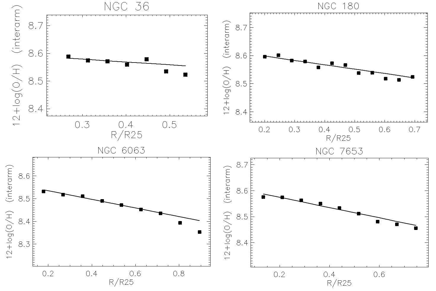
Figure 10: Radial abundance gradients in the interarm regions for our target galaxies. The squares stand for the oxygen abundances at different radii. The line shows the best fit to those data.

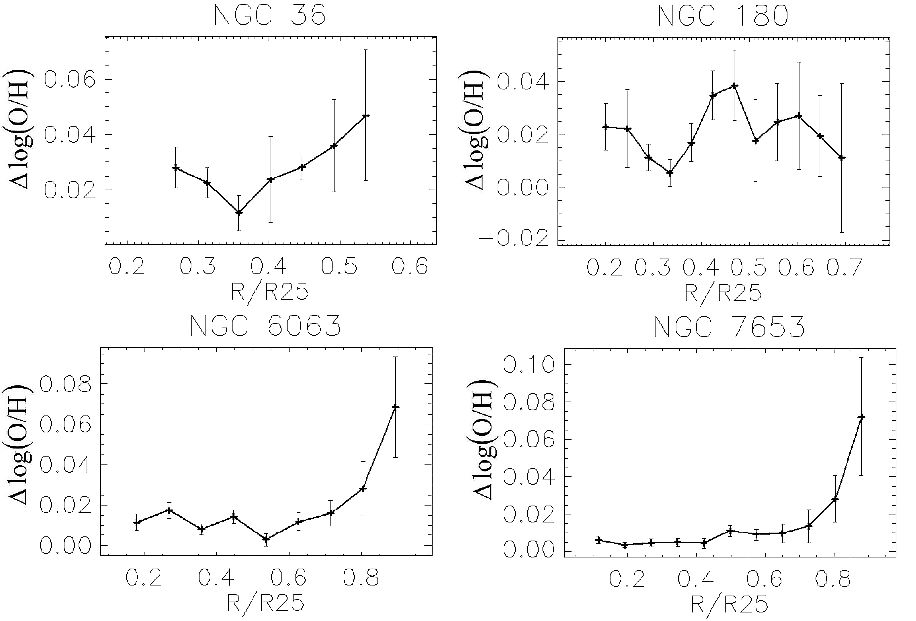
Figure 11: The enhancement of the oxygen abundance $\Delta\log$(O/H) in the spiral arms as compared to the interarm regions as a function of galactocentric distance for the target galaxies.

Table 4: The extrapolated central oxygen abundance and the slope of the oxygen abundance gradient

Galaxy	$12+\log\big{(}O/H\big{)}_{0}$	$grad$	$grad$	$R_{25}/R_{eff}$
		$dex/R_{25}$	$dex/R_{eff}$
1	2	3	4	5
NGC 36	$8.61\pm 0.01$	$-0.10\pm 0.02$	$-0.07$	1.53
NGC 180	$8.63\pm 0.01$	$-0.16\pm 0.02$	$-0.09$	1.77
NGC 6063	$8.573\pm 0.002$	$-0.189\pm 0.005$	$-0.09$	2.02
NGC 7653	$8.614\pm 0.001$	$-0.196\pm 0.003$	$-0.09$	2.15

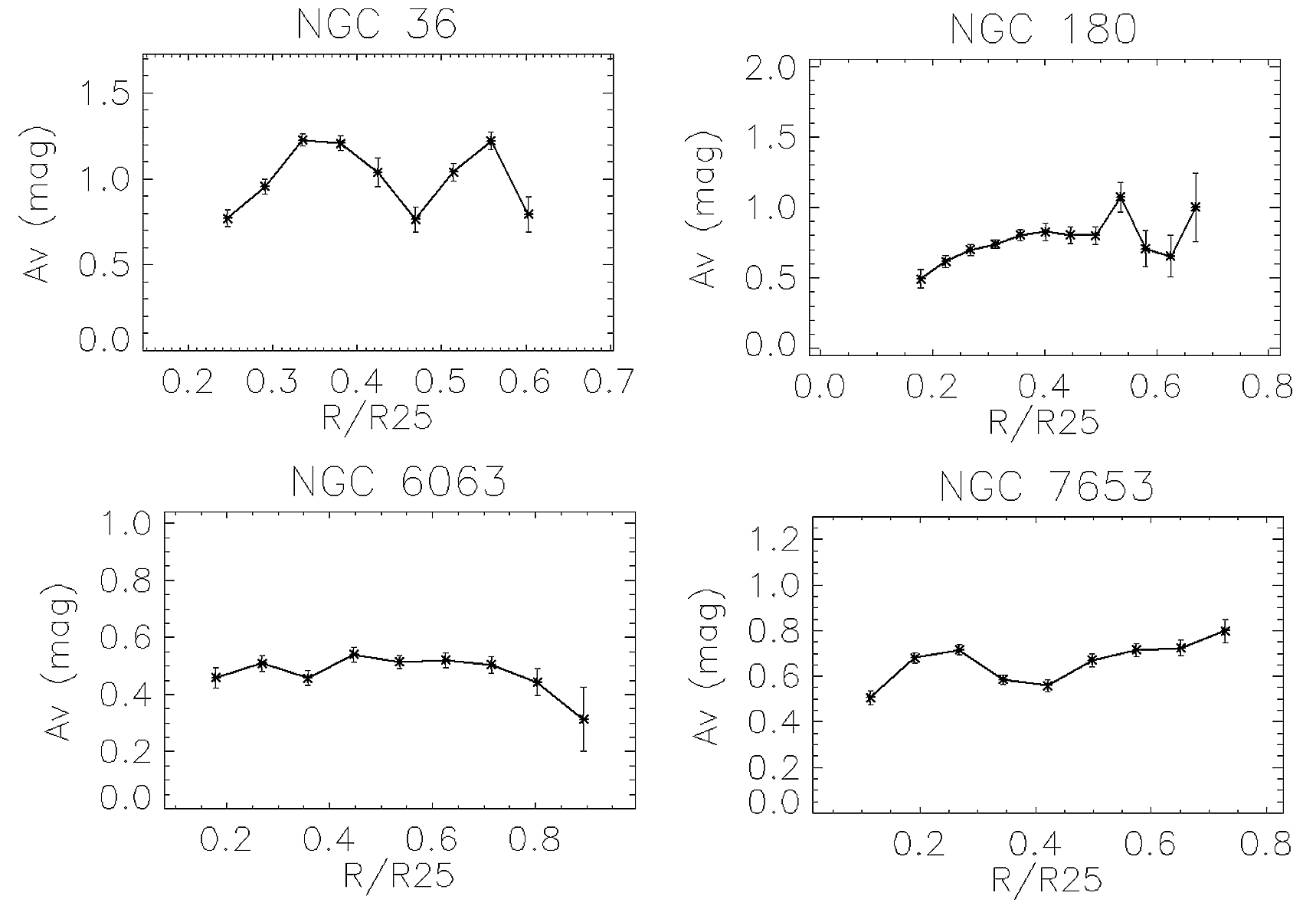
Figure 12: The visual extinction $A_{V}$ as a function of galactocentric distance in our target galaxies. The points mark the azimuthally averaged values of extinction. The error bars show the scatter.

4.3 Spiral arms in our galaxies derived from extinction maps

The method described above and used for the analysis of the abundance map to trace the spiral arms can be also applied to the extinction map. Here we search for spiral arms in our target galaxies using the Balmer decrement and succeeded in uncovering the spiral arms in each target galaxy.

Fig 12 shows the azimuthally averaged value of the visual extinction $A_{V}$ in the interarm regions as a function of galactocentric distance in our target galaxies. Inspection of Fig 12 shows that there is no common systematic change of the extinction along the radial extent of the disc; instead the extinction is constant within the uncertainties.

Fig 13 shows the difference between the extinction in the spiral arms, $A_{V}(Spiral)$, and the mean extinction in the interarm regions, $A_{V}(Interarm)$, as a function of galactocentric distance. The difference $A_{V}(Spiral)-A_{V}(Interarm)$ increases monotonically outwards.

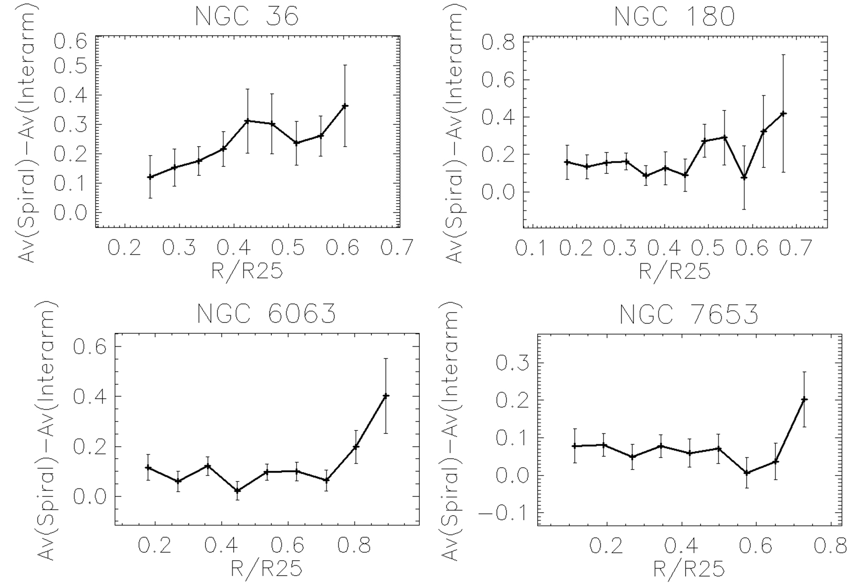
Figure 13: The difference between the total visual extinction in the spiral arms, $A_{V}(Spiral)$, and the mean extinction in the interarm regions, $A_{V}(Interarm)$, as a function of galactocentric distance.

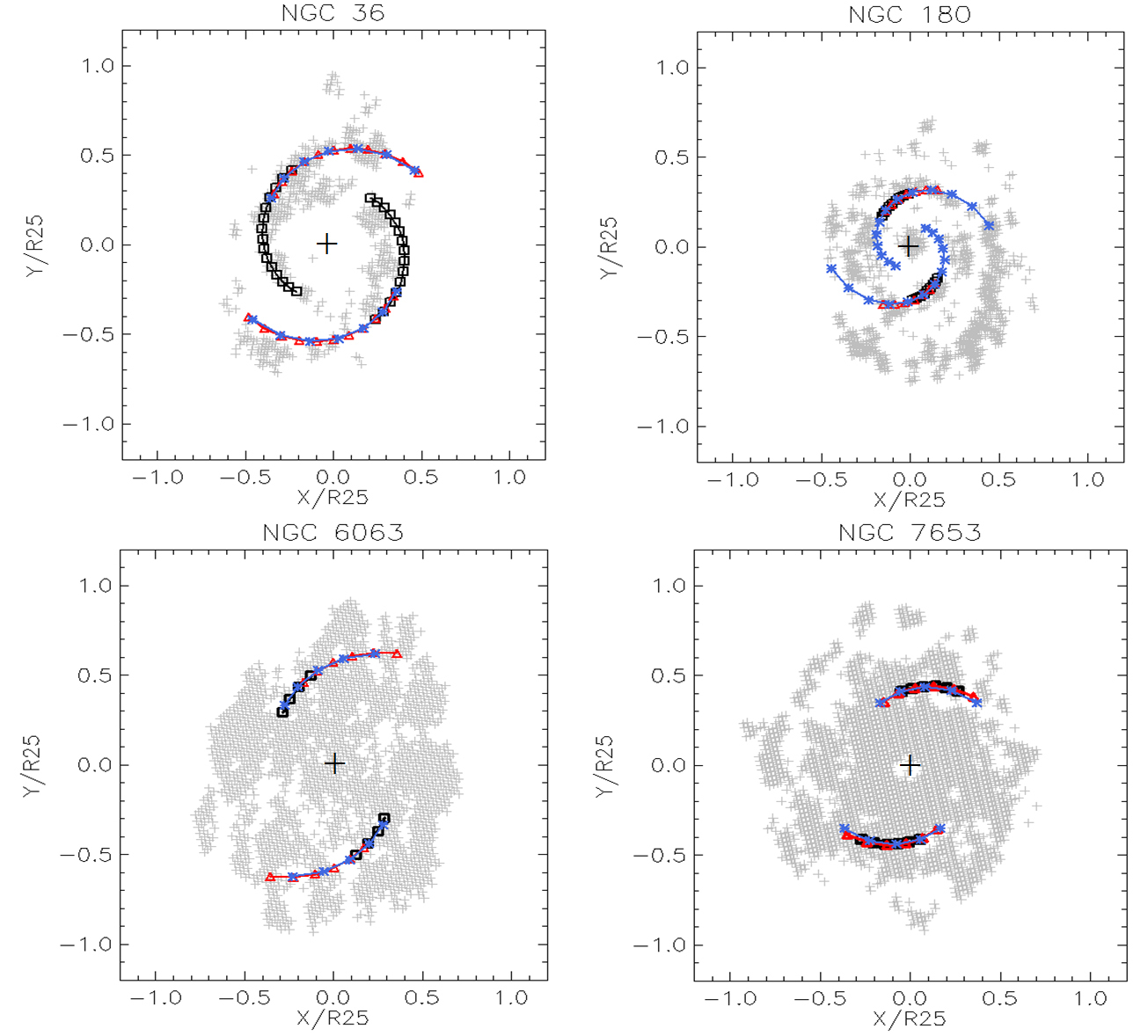
Figure 14: Comparison between spiral arms derived from the analysis of the velocity map (black squares), the extinction map (red triangles), and the oxygen abundance map (blue stars). The small grey plus signs mark the areas (pixels) with measured oxygen abundances. The large dark plus sign marks the position of the centre of the galaxy. Red rectangle shows the orientation and size of the bar in NGC 36 and NGC 180 (upper panels)

5 Discussion

Fig. 14 shows the spiral arms obtained from the maps of different tracers in the target galaxies. The spiral arms in Fig. 14 are shown within the range of galactocentric distances where they were detected (see Table 3).

Inspection of Fig. 14 (compare also the values of the pitch angle listed in Columns 6, 8, and 10 of Table 3) shows that the parameters of the spiral arms derived from maps of different tracers are in good agreement with each other. This is not surprising because of all three tracers are associated with ionized gas clouds. Since the high-density (dust) clouds are concentrated in the spiral arms one may expect a higher extinction in the spiral arms than in the interarm regions. The type II supernovae responsible for the oxygen enrichment of the interstellar gas are more often located in the spiral arms than in the interarm regions. Thus the spiral arms derived from the maps of different tracers are in line with the gravitational density wave nature of the spiral arms and the theory of the star formation. A similar conclusion has been reached by Sánchez-Menguiano et al. (2016b) on the base of the analysis of the VLT/MUSE data of the galaxy NGC 6754.

The reliability and accuracy of the parameters of the spiral arms obtained for each tracer is rather low because of the small amplitude of the disturbance of the tracer caused by the spiral arms and the relatively low spatial resolution of the observations. Moreover, a detailed photometric study and measurements of spiral arm pitch angles in 50 grand-design spiral galaxies (Savchenko & Reshetnikov, 2013) shows that about 2/3 of these galaxies demonstrate pitch angle variations exceeding 20 per cent. This also influences the accuracy of the definition of pitch angles. The fact that the parameters of the spiral arms derived from the maps of our different tracers are close to each other supports the reliability of the obtained geometrical parameters of the spiral patterns.

Sánchez-Blázquez et al. (2014) noted that the non-linear coupling between the bar and the spiral arms is an efficient mechanism for producing radial migrations across significant distances within discs. The process of radial migration should flatten the stellar metallicity gradient with time and, therefore, one can expect flatter stellar metallicity gradients in barred galaxies. It is interesting to note that the metallicity gradients expressed in terms of dex $R_{25}^{-1}$ in the barred galaxies NGC 36 and NGC 180 are flatter than in the unbarred galaxies NGC 6063 and NGC 7653. However, if the gradient is expressed in terms of dex $R_{eff}^{-1}$ then there is no difference between the gradients in barred and unbarred galaxies (Table 4). This agrees with the conclusion of Sánchez et al. (2014) and Sánchez-Blázquez et al. (2014) that there is no difference in the slope of the metallicity gradients expressed in terms of dex $R_{eff}^{-1}$ between barred and unbarred galaxies.

We found that the early-type spiral galaxies (NGC 36 and NGC 7653) demonstrate more tightly wound arms in comparison with the late-type spiral galaxies (NGC 180 and NGC 6063) as one would expect based on their morphological types. This is in agreement with previous results (e.g., Kennicutt, 1981; Savchenko & Reshetnikov, 2013).

It should be noted that Vogt et al. (2017) detected the presence of rapid abundance variations in the spiral galaxy HGC 91c based on the Multi Unit Spectroscopic Explorer (MUSE) observations. These variations can be separated in two distinct types, namely sub-kpc-scale variations associated with individual star-forming regions and kpc-scale variations correlated with the spiral structure of the galaxy. The authors conclude that the kpc-scale variations thus provide observational evidence that ISM enrichment is preferentially occurring along the spiral structure of HCG 91c, and less easily across the spiral arms.

It is known that the maximum rotation velocity, $V_{max}$, of disc galaxies correlates with the absolute blue magnitude of the galaxy $M_{B}$ and its morphological type (Rubin et al., 1980, 1982; Rubin, 1983; Burstein & Rubin, 1985). The values of the maximum rotation velocity $V_{max}$ derived in our current study (Column 5 in Table 3) are in agreement with the characteristic maximum rotation velocities for the galaxies of similar luminosity and morphological type.

We discussed in Sec. 3.6 a possible impact of the bar on the determination of the rotation curve $V_{\theta}(R)$. Through the analysis of the Fourier coefficient $b_{1}$ we found large radial velocities $V_{R}\approx(30-60)$ km s^-1 in the inner parts of both barred galaxies, while in outer part of the galaxies the radially symmetric large-scale motion is lower; $V_{R}\approx 10$ km s^-1.

The position angles of the major axis of a galaxy obtained here from the velocity field agree with the position angles determined from the analysis of the surface brightness distributions in Zinchenko et al. (2016). That is in line with the result of Barrera-Ballesteros et al. (2014), who did not find statistically significant differences between the kinematic $PA$ and the global photometric orientation of the galaxy, including barred and unbarred objects.

Fig. 6 shows a variation of the zeroth coefficient $a_{0}$ with increasing galactocentric distance in our target galaxies (the true systemic velocity is subtracted from the measured velocity of each spaxel). Such a dependence of the zeroth coefficient on the galactocentric distance was also detected by Carignan et al. (1990) in the spiral galaxy NGC 6946 and by Sakhibov & Smirnov (2004) in NGC 628. Carignan et al. (1990) assumed that the coefficient $a_{0}$ comprises just the systemic velocity of the galaxy as awhole, $V_{gal}$, and explained the radial dependence of the zeroth coefficient by the periodic variation of the inclination of the galaxy disc from $i=33^{\circ}$ up to $i=43^{\circ}$. Sakhibov & Smirnov (2004) suggested that the radial dependence of the zeroth coefficient $a_{0}$ in NGC 628 can be explained with the first mode of a density wave, which makes a contribution in zeroth harmonics. The superposition of the first and second modes can result in asymmetric spiral structure, which is apparent in the maps of the metallicity distribution of NGC 180 and NGC 7653 (Fig. 14).

Sánchez et al. (2015) and Sánchez-Menguiano et al. (2016b) considered the azimuthal distribution of the residuals of the oxygen abundance for the individual H ii regions in the galaxy NGC 6754 after subtracting the average radial gradient. They noted that the strongest residuals correspond to the spiral arms. The mean absolute value of the strongest residuals is below $\sim$0.05 dex and changes with galactocentric distance. We found a similar picture for the enhancements of the oxygen abundance in the spiral arms as shown in Fig. 11.

Sánchez-Menguiano et al. (2017) carried out a study of the arm and interarm abundance distributions in a sample of 63 CALIFA spiral galaxies. They found that the differences between the gas abundances of spiral arms and interarm regions are small and statistically significant only for flocculent and barred galaxies. The small values of the enhancement of the oxygen abundance in the spiral arms obtained here for four galaxies is in agreement with their results.

6 Conclusions

We constructed maps of the observed velocity of the ionized gas, the oxygen abundance, and the extinction (Balmer decrement) in the discs of the four spiral galaxies NGC 36, NGC 180, NGC 6063, and NGC 7653 based on integral field spectroscopy obtained by the Calar Alto Legacy Integral Field Area (CALIFA) survey. The maps were used to search for spiral arms in the discs of these galaxies via Fourier analysis. We considered non-circular motions, the enhancement of the oxygen abundance, and increased extinction as tracers of spiral arms.

The parameters of the spiral structure were obtained in all four galaxies considered and for each tracer. The pitch angles of the spiral arms obtained from the different tracers are close to each other. This strengthens the reliability of the obtained geometrical parameters of the spiral patterns although the accuracy of determination of these parameters for each tracer separately is low. The systemic velocity, inclination, position angle of the major axis, and rotation curve were also obtained for each target galaxy using the Fourier analysis of the two-dimensional velocity map.

The enhancement of the oxygen abundance in the spiral arms as compared to the abundance in the interarm regions at a given galactocentric distance is small, within a few per cent. This evidences that the influence of the spiral arms on the present-day radial abundance gradient in the discs of spiral galaxies is small and can be neglected in many tasks. There is no regular change of the extinction with galactocentric distance in the studied galaxies.

References

- Asari et al. (2007) Asari N. V., Cid Fernandes R., Stasińska G., Torres-Papaqui J. P., Mateus A., Sodré L., Schoenell W., Gomes J. M., 2007, MNRAS, 381, 263
- Barrera-Ballesteros et al. (2014) Barrera-Ballesteros J. K., et al., 2014, A&A, 568, A70
- Barrera-Ballesteros et al. (2015) Barrera-Ballesteros J. K., et al., 2015, A&A, 582, 21
- Barnes & Sellwood (2003) Barnes E. I., Sellwood J. A., 2003, AJ, 125, 1164
- Bosma (1978) Bosma A., 1978, PhD, thesis, Univ. Groningen
- Bruzual & Charlot (2003) Bruzual G., Charlot S., 2003, MNRAS, 344, 1000
- Burstein & Rubin (1985) Burstein D., Rubin V. C., 1985, ApJ, 297, 423
- Canzian (1993) Canzian B., 1993, ApJ, 414, 487
- Cardelli et al. (1989) Cardelli J. A., Clayton G. C., Mathis J. S., 1989, ApJ, 345, 245
- Carignan et al. (1990) Carignan C., Charbonneau P., Boulanger F., Viallefond F., 1990, A&A, 234, 43
- Cid Fernandes et al. (2005) Cid Fernandes R., Mateus A., Sodré L., Stasińska G., Gomes J. M., 2005, MNRAS, 358, 363
- Considere & Athanassoula (1982) Considere S., Athanassoula E., 1982, A&A, 111, 28
- Considere & Athanassoula (1988) Considere S., Athanassoula E., 1988, A&AS, 76, 365
- Elmegreen & Elmegreen (1984) Elmegreen D. M., Elmegreen B. G., 1984, ApJS, 54, 127
- Eskridge et al. (2002) Eskridge P. B., et al., 2002, ApJS, 143, 73
- Fixsen et al. (1996) Fixsen D. J., et al., 1996, ApJ, 473, 576
- Fraternali et al. (2001) Fraternali F., Oosterloo T., Sancisi R., van Moorsel G., 2001, ApJ, 562, L47
- Fridman et al. (2001a) Fridman A. M., et al., 2001a, MNRAS, 323, 651
- Fridman et al. (2001b) Fridman A. M., Khoruzhii O. V., Lyakhovich V. V., Sil’chenko O.K., Zasov A.V., Afanasiev V.L., Dodonov S,N., Boulesteix J., 2001b, A&A, 371, 538
- Frick et al. (2016) Frick P., Stepanov R., Beck R., Sokoloff D., Shukurov A., Ehle M., Lundgren A. 2015, A&A, 585, 21
- García-Benito et al. (2015) García-Benito R., et al., 2015, A&A, 576, A135
- García-Lorenzo et al. (2015) García-Lorenzo B., et al., 2015, A&A, 573, 59
- González Delgado et al. (2014) González Delgado R. M., et al., 2014, A&A, 562, A47
- González Delgado et al. (2016) González Delgado R. M., et al., 2016, A&A, 590, A44
- Grosbol et al. (1999) Grosbol P. J., Block D. L., Patsis P. A., 1999, Ap&SS, 269, 423
- Holmes et al. (2015) Holmes L., et al., 2015, MNRAS, 451, 4397
- Husemann et al. (2013) Husemann B., et al., 2013, A&A, 549, A87
- Iye et al. (1982) Iye M., Okamura S., Hamabe M., Watanabe M., 1982, ApJ, 256, 103
- Izotov et al. (1994) Izotov Y. I., Thuan T. X., Lipovetsky V. A., 1994, ApJ, 435, 647
- Kalnajs (1975) Kalnajs A. J., 1975, in Weliachew L., ed, Colloques Internationaux du Centre National de la Recherche Scientifique No. 241, La Dynamique des galaxies spirales. Editions du Centre National de la Recherche Scientifique, Paris, p. 103
- Karachentsev & Makarov (1996) Karachentsev I. D., Makarov D. A., 1996, AJ, 111, 794
- Kennicutt (1981) Kennicutt R. C. Jr., 1981, AJ, 86, 1847
- Lin et al. (1969) Lin C. C., Yuan C., Shu F. H., 1969, ApJ, 155, 721
- Martín-Navarro et al. (2015) Martín-Navarro I., et al., 2015, ApJ, 806, L31
- Mateus et al. (2006) Mateus A., Sodré L., Cid Fernandes R., Stasińska G., Schoenell W., Gomes J. M., 2006, MNRAS, 370, 721
- Mould et al. (2000) Mould J. R., Huchra J. P., Freedman W. L. et al., 2000, ApJ, 529, 786
- Nilson (1973) Nilson R., 1973, Acta Universitatis Upsalienis, Nova Regiae Societatis Upsaliensis, Series V: A Vol. 1
- Osterbrock (1989) Osterbrock D.E., 1989, Astrophysics of gaseous nebulae and active galactic nuclei. University Science Books, Mill Valley, CA
- Paturel et al. (2003) Paturel G., Petit C., Prugniel Ph., Theureau, G., Rousseau J., Brouty M., Dubois P., Chambrésy L., 2003, A&A, 412, 45
- Pérez et al. (2013) Pérez E., et al., 2013, ApJL, 764, L1
- Pilyugin et al. (2012) Pilyugin L. S., Grebel E. K., Mattsson L., 2012, MNRAS, 424, 2316
- Pilyugin et al. (2014) Pilyugin L. S., Grebel E. K., Kniazev A. Y., 2014, MNRAS, 147, 131
- Rohlfs (1977) Rohlfs K., 1977, Lectures on density wave theory. Lecture Notes in Physics Vol. 69, Springer Verlag, Berlin
- Rots (1975) Rots A. H., 1975, A&A, 45, 43
- Rubin et al. (1980) Rubin V. C., Burstein D., Thonnard N. 1980, ApJL, 242, L149
- Rubin et al. (1982) Rubin V. C., Ford W. K. Jr., Thonnard N., Burstein D., 1980, ApJ, 261, 439
- Rubin (1983) Rubin V. C., 1983, in Athanassoula E., ed, Proc. IAU Symp. 100, Internal kinematics and dynamics of galaxies. D. Reidel Publishing Co., Dordrecht, p. 3
- Sakhibov & Smirnov (1987) Sakhibov F. K., Smirnov M. A., 1987, SvA, 31, 132
- Sakhibov & Smirnov (1989) Sakhibov F. K., Smirnov M. A., 1989, SvA, 33, 476
- Sakhibov & Smirnov (1990) Sakhibov F. K., Smirnov M. A., 1990, SvA, 34, 347
- Sakhibov & Smirnov (2004) Sakhibov F. K., Smirnov M. A., 2004, Astronomy Reports, 48, 995
- Sánchez et al. (2012a) Sánchez S. F., et al., 2012a, A&A, 538, A8
- Sánchez et al. (2012b) Sánchez S. F., et al., 2012b, A&A, 546, A2
- Sánchez et al. (2014) Sánchez S. F., et al., 2014, A&A, 563, A49
- Sánchez et al. (2015) Sánchez S. F., et al., 2015, A&A, 573, A105