Comparison of Efficiencies of some Symmetry Tests around an Unknown Center

Bojana Milošević111bojana@matf.bg.ac.rs , Marko Obradović 222marcone@matf.bg.ac.rs
Faculty of Mathematics, University of Belgrade, Studenski trg 16, Belgrade, Serbia
Abstract

In this paper, some recent and classical tests of symmetry are modified for the case of an unknown center. The unknown center is estimated with its α𝛼\alpha-trimmed mean estimator. The asymptotic behavior of the new tests is explored. The local approximate Bahadur efficiency is used to compare the tests to each other as well as to some other tests.

keywords: U-statistics with estimated parameters; α𝛼\alpha-trimmed mean; asymptotic efficiency

MSC(2010): 62G10, 62G20

1 Introduction

The problem of testing symmetry has been popular for decades, mainly due to the fact that many statistical methods depend on the assumption of symmetry. The well-known examples are the robust estimators of location such as trimmed means that implicitly assume that the data come from a symmetric distribution. Another example are the bootstrap confidence intervals, that tend to converge faster when the corresponding pivotal quantity is symmetrically distributed.

Probably the most famous symmetry tests are the classical sign and Wilcoxon tests, as well as the tests proposed following the example of Kolmogorov-Smirnov and Cramer-von Mises statistics (see. [37, 13, 34]). Other examples of papers on this topic include [23, 1, 10, 11, 6, 12, 31, 27, 2].

All of these symmetry tests are designed for the case of a known center of distribution. They share many nice properties such as distribution-freeness under the null symmetry hypothesis.

There have been many attempts to adapt these tests to the case of an unknown center. Some modified Wilcoxon tests can be found in [9, 3, 4] and a modified sign test in [17].

There also exist some symmetry tests originally designed for testing symmetry around an unknown center. The famous b1subscript𝑏1\sqrt{b_{1}} test is one of the examples. Some other tests have been proposed in [29, 14, 26].

The goal of our paper is to compare some symmetry tests around an unknown center. Instead of commonly used power comparison (see e.g. [26, 38, 29, 15]), here we compare the tests using the local asymptotic efficiency. We opt for the approximate Bahadur efficiency since it is applicable to asymptotically non-normally distributed test statistics. The Bahadur efficiency of symmetry tests has been considered in, among others, [8, 25, 19, 28].

Consider the setting of testing the null hypothesis H0:θΘ0:subscript𝐻0𝜃subscriptΘ0H_{0}:\theta\in\Theta_{0} against the alternative H1:θΘ1:subscript𝐻1𝜃subscriptΘ1H_{1}:\theta\in\Theta_{1}. Let us suppose that for a test statistic Tnsubscript𝑇𝑛T_{n}, under H0subscript𝐻0H_{0}, the limit limnP{Tnt}=F(t)subscript𝑛𝑃subscript𝑇𝑛𝑡𝐹𝑡\lim_{n\rightarrow\infty}P\{T_{n}\leq t\}=F(t), where F𝐹F is non-degenerate distribution function, exists. Further, suppose that limtt2log(1F(t))=aT2subscript𝑡superscript𝑡21𝐹𝑡subscript𝑎𝑇2\lim_{t\rightarrow\infty}t^{-2}\log(1-F(t))=-\frac{a_{T}}{2}, and that the limit in probability Pθsubscript𝑃𝜃P_{\theta} limnTn=bT(θ)>0subscript𝑛subscript𝑇𝑛subscript𝑏𝑇𝜃0\lim_{n\rightarrow\infty}T_{n}=b_{T}(\theta)>0, exists for θΘ1𝜃subscriptΘ1\theta\in\Theta_{1}. The relative approximate Bahadur efficiency with respect to another test statistic Vnsubscript𝑉𝑛V_{n} is

eT,V(θ)=cT(θ)cV(θ),subscriptsuperscript𝑒𝑇𝑉𝜃subscriptsuperscript𝑐𝑇𝜃subscriptsuperscript𝑐𝑉𝜃e^{\ast}_{T,V}{(\theta)}=\frac{c^{\ast}_{T}{(\theta)}}{c^{\ast}_{V}{(\theta)}},

where

cT(θ)=aTbT2(θ)subscriptsuperscript𝑐𝑇𝜃subscript𝑎𝑇superscriptsubscript𝑏𝑇2𝜃c^{\ast}_{T}(\theta)=a_{T}b_{T}^{2}(\theta) (1)

is the approximate Bahadur slope of Tnsubscript𝑇𝑛T_{n}. Its limit when θ0𝜃0\theta\to 0 is called the local approximate Bahadur efficiency.

The tests we consider may be classified into two groups according to their limiting distributions: asymptotically normal ones; and those whose asymptotic distribution coincides with the supremum of some Gaussian process.

For the first group of tests, the coefficient aTsubscript𝑎𝑇a_{T} is the inverse of the limiting variance. For the second, it is the inverse of the supremum of the covariance function of the limiting process (see [24]).

2 Test statistics

Most of considered tests are obtained by modifying the symmetry tests around known location parameter. Let X1,..,XnX_{1},..,X_{n} be an i.i.d. sample with distribution function F𝐹F. The tests are applied to the sample shifted by the value of the location estimator. Typical choices of location estimators are the mean and the median. Here we take a more general approach, using α𝛼\alpha-trimmed means

μ(α)=112αF1(α)F1(1α)x𝑑F(x),  0<α<1/2,formulae-sequence𝜇𝛼112𝛼superscriptsubscriptsuperscript𝐹1𝛼superscript𝐹11𝛼𝑥differential-d𝐹𝑥  0𝛼12\mu(\alpha)=\frac{1}{1-2\alpha}\int_{F^{-1}(\alpha)}^{F^{-1}(1-\alpha)}xdF(x),\;\;0<\alpha<1/2,

including their boundary cases μ(0)𝜇0\mu(0) – the mean and μ(1/2)𝜇12\mu(1/2) – the median. The estimator is

μ^(α)=112αFn1(α)Fn1(1α)x𝑑Fn(x),  0<α<1/2.formulae-sequence^𝜇𝛼112𝛼superscriptsubscriptsuperscriptsubscript𝐹𝑛1𝛼superscriptsubscript𝐹𝑛11𝛼𝑥differential-dsubscript𝐹𝑛𝑥  0𝛼12\widehat{\mu}(\alpha)=\frac{1}{1-2\alpha}\int_{F_{n}^{-1}(\alpha)}^{F_{n}^{-1}(1-\alpha)}xdF_{n}(x),\;\;0<\alpha<1/2. (2)

In the case of α=0𝛼0\alpha=0 and α=1/2𝛼12\alpha=1/2, the estimators are the sample mean and the sample median, respectively.

The modified statistics we consider in this paper are:

  • Modified sign test

    S=1ni=1nI{Xjμ^(α)>0}12;S1𝑛superscriptsubscript𝑖1𝑛Isubscript𝑋𝑗^𝜇𝛼012{\rm S}=\frac{1}{n}\sum_{i=1}^{n}{\rm I}\{X_{j}-\widehat{\mu}(\alpha)>0\}-\frac{1}{2};
  • Modified Wilcoxon test

    W=1(n2)1i<jnI{Xi+Xj2μ^(α)>0}12;W1binomial𝑛2subscript1𝑖𝑗𝑛Isubscript𝑋𝑖subscript𝑋𝑗2^𝜇𝛼012{\rm W}=\frac{1}{\binom{n}{2}}\sum_{1\leq i<j\leq n}{\rm I}\{X_{i}+X_{j}-2\widehat{\mu}(\alpha)>0\}-\frac{1}{2};
  • Modified Kolmogorov-Smirnov symmetry test

    KS=supt|Fn(t+μ^(α))+Fn(μ^(α)t)1|;KSsubscriptsupremum𝑡subscript𝐹𝑛𝑡^𝜇𝛼subscript𝐹𝑛^𝜇𝛼𝑡1{\rm KS}=\sup_{t}|F_{n}(t+\widehat{\mu}(\alpha))+F_{n}(\widehat{\mu}(\alpha)-t)-1|;
  • Modified tests based on the Baringhaus-Henze characterization (see [7, 22])

    BHIsuperscriptBH𝐼\displaystyle{\rm BH}^{I} =1n(n2)i3=1n𝒞2(12I{|Xi1μ^(α)|<|Xi3μ^(α)|}+12I{|Xi2μ^(α)|<|Xi3μ^(α)|}\displaystyle=\frac{1}{n\binom{n}{2}}\sum_{i_{3}=1}^{n}\sum_{\mathcal{C}_{2}}\Big{(}\frac{1}{2}{\rm I}\{|X_{i_{1}}-\widehat{\mu}(\alpha)|<|X_{i_{3}}-\widehat{\mu}(\alpha)|\}+\frac{1}{2}{\rm I}\{|X_{i_{2}}-\widehat{\mu}(\alpha)|<|X_{i_{3}}-\widehat{\mu}(\alpha)|\}
    I{|X2;Xi1,Xi2μ^(α)|<|Xi3μ^(α)|});\displaystyle-{\rm I}\{|X_{2;X_{i_{1}},X_{i_{2}}}-\widehat{\mu}(\alpha)|<|X_{i_{3}}-\widehat{\mu}(\alpha)|\}\Big{)};
    BHKsuperscriptBH𝐾\displaystyle{\rm BH}^{K} =supt>0|1(n2)𝒞2(12I{|Xi1μ^(α)|<|Xi3μ^(α)|}+12I{|Xi2μ^(α)|<|Xi3μ^(α)|}\displaystyle=\sup_{t>0}\Big{|}\frac{1}{\binom{n}{2}}\sum_{\mathcal{C}_{2}}\Big{(}\frac{1}{2}{\rm I}\{|X_{i_{1}}-\widehat{\mu}(\alpha)|<|X_{i_{3}}-\widehat{\mu}(\alpha)|\}+\frac{1}{2}{\rm I}\{|X_{i_{2}}-\widehat{\mu}(\alpha)|<|X_{i_{3}}-\widehat{\mu}(\alpha)|\}
    I{|X2;Xi1,Xi2μ^(α)|<t})|;\displaystyle-{\rm I}\{|X_{2;X_{i_{1}},X_{i_{2}}}-\widehat{\mu}(\alpha)|<t\}\Big{)}\Big{|};
  • Modified tests based on the Ahsanullah’s characterization (see [31])

    NAI(k)superscriptNA𝐼𝑘\displaystyle{\rm NA}^{I}(k) =1n(nk)ik+1=1n𝒞k(I{|X1;Xi1,,Xikμ^(α)|<|Xik+1μ^(α)|}\displaystyle=\frac{1}{n\binom{n}{k}}\sum_{i_{k+1}=1}^{n}\sum_{\mathcal{C}_{k}}\Big{(}{\rm I}\{|X_{1;X_{i_{1}},\ldots,X_{i_{k}}}-\widehat{\mu}(\alpha)|<|X_{i_{k+1}}-\widehat{\mu}(\alpha)|\}
    I{|Xk;Xi1,,Xikμ^(α)|<|Xik+1μ^(α)|});\displaystyle-{\rm I}\{|X_{k;X_{i_{1}},\ldots,X_{i_{k}}}-\widehat{\mu}(\alpha)|<|X_{i_{k+1}}-\widehat{\mu}(\alpha)|\}\Big{)};
    NAK(k)superscriptNA𝐾𝑘\displaystyle{\rm NA}^{K}(k) =supt>0|1(nk)𝒞k(I{|X1;Xi1,,Xikμ^(α)|<t}\displaystyle=\sup_{t>0}\Big{|}\frac{1}{\binom{n}{k}}\sum_{\mathcal{C}_{k}}\Big{(}{\rm I}\{|X_{1;X_{i_{1}},\ldots,X_{i_{k}}}-\widehat{\mu}(\alpha)|<t\}
    I{|Xk;Xi1,,Xikμ^(α)|<t})|;\displaystyle-{\rm I}\{|X_{k;X_{i_{1}},\ldots,X_{i_{k}}}-\widehat{\mu}(\alpha)|<t\}\Big{)}\Big{|};
  • Modified tests based on the Milošević-Obradović characterization (see [27])

    MOI(k)superscriptMO𝐼𝑘\displaystyle{\rm MO}^{I}(k) =1n(n2k)i2k+1=1n𝒞2k(I{|Xk;Xi1,,Xi2kμ^(α)|<|Xi2k+1μ^(α)|}\displaystyle=\frac{1}{n\binom{n}{2k}}\sum_{i_{2k+1}=1}^{n}\sum_{\mathcal{C}_{2k}}\Big{(}{\rm I}\{|X_{k;X_{i_{1}},\ldots,X_{i_{2k}}}-\widehat{\mu}(\alpha)|<|X_{i_{2k+1}}-\widehat{\mu}(\alpha)|\}
    I{|Xk+1;Xi1,,Xi2kμ^(α)|<|Xi2k+1μ^(α)|});\displaystyle-{\rm I}\{|X_{k+1;X_{i_{1}},\ldots,X_{i_{2k}}}-\widehat{\mu}(\alpha)|<|X_{i_{2k+1}}-\widehat{\mu}(\alpha)|\}\Big{)};
    MOK(k)superscriptMO𝐾𝑘\displaystyle{\rm MO}^{K}(k) =supt>0|1(nk)𝒞2k(I{|Xk;Xi1,,Xi2kμ^(α)|<t}\displaystyle=\sup_{t>0}\Big{|}\frac{1}{\binom{n}{k}}\sum_{\mathcal{C}_{2k}}\Big{(}{\rm I}\{|X_{k;X_{i_{1}},\ldots,X_{i_{2k}}}-\widehat{\mu}(\alpha)|<t\}
    I{|Xk+1;Xi1,,Xi2kμ^(α)|<t})|,\displaystyle-{\rm I}\{|X_{k+1;X_{i_{1}},\ldots,X_{i_{2k}}}-\widehat{\mu}(\alpha)|<t\}\Big{)}\Big{|},

where Xk;Xi1,Ximsubscript𝑋𝑘subscript𝑋subscript𝑖1subscript𝑋subscript𝑖𝑚X_{k;X_{i_{1}},...X_{i_{m}}} stands for the k𝑘kth order statistic of the subsample Xi1,,Ximsubscript𝑋subscript𝑖1subscript𝑋subscript𝑖𝑚X_{i_{1}},...,X_{i_{m}}, and 𝒞m={(i1,,im):1i1<<imn}subscript𝒞𝑚conditional-setsubscript𝑖1subscript𝑖𝑚1subscript𝑖1subscript𝑖𝑚𝑛\mathcal{C}_{m}=\{(i_{1},\ldots,i_{m}):1\leq i_{1}<\cdots<i_{m}\leq n\}.

Note that NAI(2)superscriptNA𝐼2{\rm NA}^{I}(2) and MOI(1)superscriptMO𝐼1{\rm MO}^{I}(1) coincide. The same holds for NAK(2)superscriptNA𝐾2{\rm NA}^{K}(2) and MOK(1)superscriptMO𝐾1{\rm MO}^{K}(1).

Among the tests originally intended for testing symmetry around an unknown mean, the most famous is classical b1subscript𝑏1\sqrt{b_{1}} test, based on the sample skewness coefficient, with test statistic

b1=m^3s3,subscript𝑏1subscript^𝑚3superscript𝑠3\sqrt{b_{1}}=\frac{\hat{m}_{3}}{s^{3}}, (3)

where m^3subscript^𝑚3\hat{m}_{3} is the sample third central moment and s𝑠s is sample standard deviation. The test is applicable if the sample comes from a distribution with finite sixth moment.

We also consider the class of tests based on so-called Bonferoni measure. In [14] the following test statistic is proposed:

CM=X¯M^s,CM¯𝑋^𝑀𝑠{\rm CM}=\frac{\bar{X}-\hat{M}}{s},

where M^^𝑀\hat{M} is the sample median and s𝑠s is the sample standard deviation. Similar tests are proposed in [29] and [26], with the following statistic

γ=2(X¯M^)𝛾2¯𝑋^𝑀\displaystyle\gamma=2(\bar{X}-\hat{M})
MGG=X¯M^J,where J=π21ni=1n|XiM^|.formulae-sequenceMGG¯𝑋^𝑀𝐽where 𝐽𝜋21𝑛superscriptsubscript𝑖1𝑛subscript𝑋𝑖^𝑀\displaystyle{\rm MGG}=\frac{\bar{X}-\hat{M}}{J},\;\;\text{where }J=\sqrt{\frac{\pi}{2}}\frac{1}{n}\sum_{i=1}^{n}|X_{i}-\hat{M}|.

These tests are applicable if the sample comes from a distribution with finite second moment.

For the supremum-type tests, we consider large values of test statistic to be significant. For others, which are asymptotically normally distributed, we consider large absolute values of tests statistic to be significant.

3 Bahadur approximate Slopes

We can divide the considered test statistics into three groups based on their structure:

  • non-degenerate U-statistics with estimated parameters;

  • the suprema of families of non-degenerate (in sense of [30]) U-statistics with estimated parameters;

  • other statistics with limiting normal distribution.

Since we are dealing with U-statistics with estimated location parameters, we shall examine their limiting distribution using the technique from [33]. With this in mind, we give the following definition.

Definition 3.1

Let 𝒰𝒰\mathcal{U} be the family of U-statistics Un(μ)subscript𝑈𝑛𝜇U_{n}(\mu), with bounded symmetric kernel Φ(;μ)Φ𝜇\Phi(\cdot;\mu), that satisfy the following conditions:

  • EUn(μ)=0𝐸subscript𝑈𝑛𝜇0EU_{n}(\mu)=0;

  • nUn𝑛subscript𝑈𝑛\sqrt{n}U_{n} converges to normal distribution whose variance does not depend on μ𝜇\mu;

  • For K(μ,d)𝐾𝜇𝑑K(\mu,d), a neighbourhood of μ𝜇\mu of a radius d𝑑d, there exists a constant C>0𝐶0C>0, such that, if μK(μ,d)superscript𝜇𝐾𝜇𝑑\mu^{\prime}\in K(\mu,d) then

    E(supμK(μ,d)|Φ(;μ)Φ(;μ)|)Cd.𝐸subscriptsupremumsuperscript𝜇𝐾𝜇𝑑Φsuperscript𝜇Φ𝜇𝐶𝑑E\big{(}\sup_{\mu^{\prime}\in K(\mu,d)}|\Phi(\cdot;\mu^{\prime})-\Phi(\cdot;\mu)|\big{)}\leq Cd.

All our U-statistics belong to this family due to unbiasedness, non-degeneracy and uniform boundness of their kernels.

Since our comparison tool is the local asymptotic efficiency, we are going to consider alternatives close to some symmetric distribution. Therefore, we define the family of close alternatives that satisfy some regularity conditions (see also [32]).

Definition 3.2

Let 𝒢={G(x;θ)}𝒢𝐺𝑥𝜃\mathcal{G}=\{G(x;\theta)\} be the family of absolutely continuous distribution functions, with densities g(x;θ)𝑔𝑥𝜃g(x;\theta), satisfying the following conditions:

  • g(x;θ)𝑔𝑥𝜃g(x;\theta) is symmetric around some location parameter μ𝜇\mu if and only if θ=0𝜃0\theta=0;

  • g(x;θ)𝑔𝑥𝜃g(x;\theta) is twice continuously differentiable along θ𝜃\theta in some neighbourhood of zero;

  • all second derivatives of g(x;θ)𝑔𝑥𝜃g(x;\theta) exist and are absolutely integrable for θ𝜃\theta in some neighbourhood of zero.

For brevity, in what follows, we shall use the following notation:

F(x):=G(x,0);f(x):=g(x,0);H(x):=Gθ(x,0);h(x):=gθ(x,0).formulae-sequenceassign𝐹𝑥𝐺𝑥0formulae-sequenceassign𝑓𝑥𝑔𝑥0formulae-sequenceassign𝐻𝑥subscriptsuperscript𝐺𝜃𝑥0assign𝑥subscriptsuperscript𝑔𝜃𝑥0\displaystyle F(x):=G(x,0);\;\;f(x):=g(x,0);\;\;H(x):=G^{\prime}_{\theta}(x,0);\;\;h(x):=g^{\prime}_{\theta}(x,0).

The null hypothesis of symmetry can now be expressed as: H0:θ=0.:subscript𝐻0𝜃0H_{0}:\theta=0. To calculate the local approximate slope (1), we need to find the variance of the limiting normal distribution under the null hypothesis, as well as the limit in probability under a close alternative. We achieve this goal using the following two theorems.

Theorem 3.3

Let 𝐗=(X1,X2,Xn)𝐗subscript𝑋1subscript𝑋2subscript𝑋𝑛\boldsymbol{X}=(X_{1},X_{2}...,X_{n}) be an i.i.d. sample from an absolutely continuous symmetric distribution, with distribution function F𝐹F. Let Un(μ)subscript𝑈𝑛𝜇U_{n}(\mu) with kernel Φ(𝐗;μ)Φ𝐗𝜇\Phi(\boldsymbol{X};\mu) be a U𝑈U-statistic of order m𝑚m from the family 𝒰𝒰\mathcal{U}; and let μ^(α)^𝜇𝛼\widehat{\mu}(\alpha), 0α1/20𝛼120\leq\alpha\leq 1/2, be the α𝛼\alpha-trimmed sample mean (2). Then nUn(μ^(α))𝑛subscript𝑈𝑛^𝜇𝛼\sqrt{n}U_{n}(\widehat{\mu}(\alpha)) converges in distribution to a zero mean normal random variable with the following variance:

σU,F2(α)subscriptsuperscript𝜎2𝑈𝐹𝛼\displaystyle\sigma^{2}_{U,F}(\alpha) =m2(φ2(x)f(x)dx+2(12α)2(φ(x)f(x)dx)2\displaystyle=m^{2}\Bigg{(}\int_{-\infty}^{\infty}\varphi^{2}(x)f(x)dx+\frac{2}{(1-2\alpha)^{2}}\bigg{(}\int_{-\infty}^{\infty}\varphi(x)f^{\prime}(x)dx\bigg{)}^{2}
(0q1αx2f(x)𝑑x+α(q1α)2)+412α(φ(x)f(x)𝑑x)absentsuperscriptsubscript0subscript𝑞1𝛼superscript𝑥2𝑓𝑥differential-d𝑥𝛼superscriptsubscript𝑞1𝛼2412𝛼superscriptsubscript𝜑𝑥superscript𝑓𝑥differential-d𝑥\displaystyle\cdot\bigg{(}\int_{0}^{q_{1-\alpha}}x^{2}f(x)dx+\alpha(q_{1-\alpha})^{2}\bigg{)}+\frac{4}{1-2\alpha}\bigg{(}\int_{-\infty}^{\infty}\varphi(x)f^{\prime}(x)dx\bigg{)}
(0q1αφ(x)xf(x)dx+q1αq1αφ(x)f(x)dx)),\displaystyle\cdot\bigg{(}\int_{0}^{q_{1-\alpha}}\varphi(x)xf(x)dx+q_{1-\alpha}\int_{q_{1-\alpha}}^{\infty}\varphi(x)f(x)dx\bigg{)}\Bigg{)},

for 0<α<1/20𝛼120<\alpha<1/2, where φ(x)=E(Φ(𝕏;μ)|X1=x)𝜑𝑥𝐸conditionalΦ𝕏𝜇subscript𝑋1𝑥\varphi(x)=E(\Phi(\mathbb{X};\mu)|X_{1}=x) is the first projection of the kernel Φ(𝕏;μ)Φ𝕏𝜇\Phi(\mathbb{X};\mu) on a basic observation, and q1α=F1(1α)subscript𝑞1𝛼superscript𝐹11𝛼q_{1-\alpha}=F^{-1}(1-\alpha) is the (1α)1𝛼(1-\alpha)th quantile of F.

In the case of boundary values of α𝛼\alpha, the expression above becomes:

σU,F2(0)subscriptsuperscript𝜎2𝑈𝐹0\displaystyle\sigma^{2}_{U,F}(0) =m2(φ2(x)f(x)dx+2(φ(x)f(x)dx)2(0x2f(x)dx)\displaystyle=m^{2}\Bigg{(}\int_{-\infty}^{\infty}\varphi^{2}(x)f(x)dx+2\bigg{(}\int_{-\infty}^{\infty}\varphi(x)f^{\prime}(x)dx\bigg{)}^{2}\bigg{(}\int_{0}^{\infty}x^{2}f(x)dx\bigg{)}
+4(φ(x)f(x)dx)(0φ(x)xf(x)dx)),\displaystyle+4\bigg{(}\int_{-\infty}^{\infty}\varphi(x)f^{\prime}(x)dx\bigg{)}\cdot\bigg{(}\int_{0}^{\infty}\varphi(x)xf(x)dx\bigg{)}\Bigg{)},

and

σU,F2(1/2)subscriptsuperscript𝜎2𝑈𝐹12\displaystyle\sigma^{2}_{U,F}(1/2) =m2(φ2(x)f(x)dx+14f2(0)(φ(x)f(x)dx)2\displaystyle=m^{2}\Bigg{(}\int_{-\infty}^{\infty}\varphi^{2}(x)f(x)dx+\frac{1}{4f^{2}(0)}\bigg{(}\int_{-\infty}^{\infty}\varphi(x)f^{\prime}(x)dx\bigg{)}^{2}
+2f(0)(φ(x)f(x)dx)(0φ(x)f(x)dx)).\displaystyle+\frac{2}{f(0)}\bigg{(}\int_{-\infty}^{\infty}\varphi(x)f^{\prime}(x)dx\bigg{)}\cdot\bigg{(}\int_{0}^{\infty}\varphi(x)f(x)dx\bigg{)}\Bigg{)}.

Proof. We prove only the case 0<α<0.50𝛼0.50<\alpha<0.5. The rest are analogous and simpler.

Notice that μ^(α)^𝜇𝛼\hat{\mu}(\alpha) has its Bahadur representation [35]

μ^(α)μ(α)=1nj=1nψα,F(Xj)+Rn,^𝜇𝛼𝜇𝛼1𝑛superscriptsubscript𝑗1𝑛subscript𝜓𝛼𝐹subscript𝑋𝑗subscript𝑅𝑛\hat{\mu}(\alpha)-\mu(\alpha)=\frac{1}{n}\sum_{j=1}^{n}\psi_{\alpha,F}(X_{j})+R_{n}, (4)

where

ψα,F(x)=112αα1αtI{x<F1(t)}f(F1)(t)𝑑tsubscript𝜓𝛼𝐹𝑥112𝛼superscriptsubscript𝛼1𝛼𝑡𝐼𝑥superscript𝐹1𝑡𝑓superscript𝐹1𝑡differential-d𝑡\psi_{\alpha,F}(x)=\frac{1}{1-2\alpha}\int_{\alpha}^{1-\alpha}\frac{t-I\{x<F^{-1}(t)\}}{f(F^{-1})(t)}dt

is the influence curve of μ(α)𝜇𝛼\mu(\alpha), and nRn𝑛subscript𝑅𝑛\sqrt{n}R_{n} converges in probability to zero.

Using the multivariate central limit theorem for U-statistics we conclude that the joint limiting distribution of nUn𝑛subscript𝑈𝑛\sqrt{n}U_{n} and n(μ^(α)μ(α))𝑛^𝜇𝛼𝜇𝛼\sqrt{n}(\hat{\mu}(\alpha)-\mu(\alpha)) is bivariate normal 𝒩2(𝟎,Σ)subscript𝒩20Σ\mathcal{N}_{2}(\boldsymbol{0},\Sigma), where

Σ=(m2φ2(x)𝑑F(x)mψα,F(x)φ(x)𝑑F(x)mψα,F(x)φ(x)𝑑F(x)ψα,F2(x)𝑑F(x)).Σsuperscript𝑚2superscriptsubscriptsuperscript𝜑2𝑥differential-d𝐹𝑥𝑚superscriptsubscriptsubscript𝜓𝛼𝐹𝑥𝜑𝑥differential-d𝐹𝑥𝑚superscriptsubscriptsubscript𝜓𝛼𝐹𝑥𝜑𝑥differential-d𝐹𝑥superscriptsubscriptsubscriptsuperscript𝜓2𝛼𝐹𝑥differential-d𝐹𝑥\Sigma=\left(\begin{array}[]{cc}m^{2}\int_{-\infty}^{\infty}\varphi^{2}(x)dF(x)&m\int_{-\infty}^{\infty}\psi_{\alpha,F}(x)\varphi(x)dF(x)\\ m\int_{-\infty}^{\infty}\psi_{\alpha,F}(x)\varphi(x)dF(x)&\int_{-\infty}^{\infty}\psi^{2}_{\alpha,F}(x)dF(x)\end{array}\right).

Therefore, the conditions 2.3 and 2.9B of [33, Theorem 2.13] are satisfied. Hence we have nUn(μ^(α))𝑑𝒩(0,σU,F2(α))𝑛subscript𝑈𝑛^𝜇𝛼𝑑𝒩0subscriptsuperscript𝜎2𝑈𝐹𝛼\sqrt{n}U_{n}(\widehat{\mu}(\alpha))\overset{d}{\rightarrow}\mathcal{N}(0,\sigma^{2}_{U,F}(\alpha)) where

σU,F2(α)=[1,A]TΣ[1,A], and A=EγΦ(;μ)μ|μ=γ=mφ(x)f(x)𝑑x.formulae-sequencesubscriptsuperscript𝜎2𝑈𝐹𝛼superscript1𝐴𝑇Σ1𝐴 and 𝐴evaluated-atsubscript𝐸𝛾Φsubscriptsuperscript𝜇𝜇𝜇𝛾𝑚superscriptsubscript𝜑𝑥superscript𝑓𝑥differential-d𝑥\displaystyle\sigma^{2}_{U,F}(\alpha)=[1,A]^{T}\Sigma[1,A],\text{ and }A=E_{\gamma}\Phi(\cdot;\mu)^{{}^{\prime}}_{\mu}\Big{|}_{\mu=\gamma}=m\int_{-\infty}^{\infty}\varphi(x)f^{\prime}(x)dx.

\Box

Theorem 3.4

Under the same assumptions as in Theorem 3.3, the limit in probability of the modified statistic Un(μ^(α))subscript𝑈𝑛^𝜇𝛼U_{n}(\widehat{\mu}(\alpha)) under alternative g(x;θ)𝒢𝑔𝑥𝜃𝒢g(x;\theta)\in\mathcal{G} is

b(θ,α)=mφ(x)(h(x)+μθ(0,α)f(x))𝑑xθ+o(θ),𝑏𝜃𝛼𝑚superscriptsubscript𝜑𝑥𝑥subscriptsuperscript𝜇𝜃0𝛼superscript𝑓𝑥differential-d𝑥𝜃𝑜𝜃\displaystyle b(\theta,\alpha)=m\int_{-\infty}^{\infty}\varphi(x)(h(x)+\mu^{\prime}_{\theta}(0,\alpha)f^{\prime}(x))dx\cdot\theta+o(\theta),

where μθ(0,α)=112α(q1α(H(q1α)+H(q1α))+q1αq1αxh(x)𝑑x)subscriptsuperscript𝜇𝜃0𝛼112𝛼subscript𝑞1𝛼𝐻subscript𝑞1𝛼𝐻subscript𝑞1𝛼superscriptsubscriptsubscript𝑞1𝛼subscript𝑞1𝛼𝑥𝑥differential-d𝑥\mu^{\prime}_{\theta}(0,\alpha)=\frac{1}{1-2\alpha}\bigg{(}-q_{1-\alpha}\Big{(}H(q_{1-\alpha})+H(-q_{1-\alpha})\Big{)}+\int_{-q_{1-\alpha}}^{q_{1-\alpha}}xh(x)dx\bigg{)}, for 0<α<1/20𝛼120<\alpha<1/2, μθ(0,1/2)=H(0)/f(0)subscriptsuperscript𝜇𝜃012𝐻0𝑓0\mu^{\prime}_{\theta}(0,1/2)=-H(0)/f(0), and μθ(0,0)=xh(x)𝑑xsubscriptsuperscript𝜇𝜃00superscriptsubscript𝑥𝑥differential-d𝑥\mu^{\prime}_{\theta}(0,0)=\int_{-\infty}^{\infty}xh(x)dx.

Proof.Let L(𝒙;θ)𝐿𝒙𝜃L(\boldsymbol{x};\theta) be the likelihood function of the sample. Using the law of large numbers for U𝑈U-statistics with estimated parameters (see [20]), the limit in probability of Un(μ^(α))subscript𝑈𝑛^𝜇𝛼U_{n}(\widehat{\mu}(\alpha)) is

b(θ,α)𝑏𝜃𝛼\displaystyle b(\theta,\alpha) =Φ(𝒙μ(θ,α))L(𝒙;θ)𝑑𝒙absentsuperscriptsubscriptΦ𝒙𝜇𝜃𝛼𝐿𝒙𝜃differential-d𝒙\displaystyle=\int_{-\infty}^{\infty}\Phi(\boldsymbol{x}-\mu(\theta,\alpha))L(\boldsymbol{x};\theta)d\boldsymbol{x}
=Φ(𝒙)L(𝒙+μ(θ,α);θ)𝑑𝒙absentsuperscriptsubscriptΦ𝒙𝐿𝒙𝜇𝜃𝛼𝜃differential-d𝒙\displaystyle=\int_{-\infty}^{\infty}\Phi(\boldsymbol{x})L(\boldsymbol{x}+\mu(\theta,\alpha);\theta)d\boldsymbol{x}
=Φ(𝒙)i=1ng(xi+μ(θ,α);θ)d𝒙.absentsuperscriptsubscriptΦ𝒙superscriptsubscriptproduct𝑖1𝑛𝑔subscript𝑥𝑖𝜇𝜃𝛼𝜃𝑑𝒙\displaystyle=\int_{-\infty}^{\infty}\Phi(\boldsymbol{x})\prod_{i=1}^{n}g(x_{i}+\mu(\theta,\alpha);\theta)d\boldsymbol{x}.

The first derivative with respect to θ𝜃\theta at θ=0𝜃0\theta=0 is

b(0,α)superscript𝑏0𝛼\displaystyle b^{\prime}(0,\alpha) =Φ(𝒙)[j=1n(μ(0,α)f(xj)+h(xj))i=1ijnf(xi)]𝑑𝒙absentsuperscriptsubscriptΦ𝒙delimited-[]superscriptsubscript𝑗1𝑛superscript𝜇0𝛼superscript𝑓subscript𝑥𝑗subscript𝑥𝑗superscriptsubscriptproduct𝑖𝑗𝑖1𝑛𝑓subscript𝑥𝑖differential-d𝒙\displaystyle=\int_{-\infty}^{\infty}\Phi(\boldsymbol{x})\Big{[}\sum_{j=1}^{n}(\mu^{\prime}(0,\alpha)f^{\prime}(x_{j})+h(x_{j}))\prod_{\underset{i\neq j}{i=1}}^{n}f(x_{i})\Big{]}d\boldsymbol{x}
=mφ(x)((μ(0,α)f(x)+h(x))dx.\displaystyle=m\int_{-\infty}^{\infty}\varphi(x)((\mu^{\prime}(0,\alpha)f^{\prime}(x)+h(x))dx.

Expanding b(θ,α)𝑏𝜃𝛼b(\theta,\alpha) in the Maclaurin series we complete the proof. \Box

In the case of supremum-type statistics, the following two theorems, analogous to the Theorem 3.3 and Theorem 3.4, are used.

Theorem 3.5

Let 𝐗=(X1,X2,Xn)𝐗subscript𝑋1subscript𝑋2subscript𝑋𝑛\boldsymbol{X}=(X_{1},X_{2}...,X_{n}) be an i.i.d. sample from an absolutely continuous symmetric distribution, with function F𝐹F. Let {Un(μ;t)}subscript𝑈𝑛𝜇𝑡\{U_{n}(\mu;t)\} be a non-degenerate family of U-statistics of order m𝑚m with kernel Φ(;t)Φ𝑡\Phi(\cdot;t), that belong to the family 𝒰𝒰\mathcal{U}; and let μ^(α)^𝜇𝛼\widehat{\mu}(\alpha), 0α0.50𝛼0.50\leq\alpha\leq 0.5, be the α𝛼\alpha-trimmed sample mean (2). Then the family {Un(μ^(α);t)}subscript𝑈𝑛^𝜇𝛼𝑡\{U_{n}(\widehat{\mu}(\alpha);t)\} is also non-degenerate with the variance function

σU,F2(α;t)subscriptsuperscript𝜎2𝑈𝐹𝛼𝑡\displaystyle\sigma^{2}_{U,F}(\alpha;t) =m2(φ2(x;t)f(x)dx+(φ(x;t)f(x)dx)22(12α)2\displaystyle=m^{2}\Bigg{(}\int_{-\infty}^{\infty}\varphi^{2}(x;t)f(x)dx+\bigg{(}\int_{-\infty}^{\infty}\varphi(x;t)f^{\prime}(x)dx\bigg{)}^{2}\frac{2}{(1-2\alpha)^{2}}
(0q1αx2f(x)𝑑x+α(q1α)2)+412α(φ(x;t)f(x)𝑑x)absentsuperscriptsubscript0subscript𝑞1𝛼superscript𝑥2𝑓𝑥differential-d𝑥𝛼superscriptsubscript𝑞1𝛼2412𝛼superscriptsubscript𝜑𝑥𝑡superscript𝑓𝑥differential-d𝑥\displaystyle\cdot\bigg{(}\int_{0}^{q_{1-\alpha}}x^{2}f(x)dx+\alpha(q_{1-\alpha})^{2}\bigg{)}+\frac{4}{1-2\alpha}\bigg{(}\int_{-\infty}^{\infty}\varphi(x;t)f^{\prime}(x)dx\bigg{)}
(0q1αφ(x;t)xf(x)dx+q1αq1αφ(x;t)f(x)dx)),\displaystyle\cdot\bigg{(}\int_{0}^{q_{1-\alpha}}\varphi(x;t)xf(x)dx+q_{1-\alpha}\int_{q_{1-\alpha}}^{\infty}\varphi(x;t)f(x)dx\bigg{)}\Bigg{)},

for 0<α<1/20𝛼120<\alpha<1/2. In the case of boundary values of α𝛼\alpha, we have

σU,F2(0;t)subscriptsuperscript𝜎2𝑈𝐹0𝑡\displaystyle\sigma^{2}_{U,F}(0;t) =m2(φ2(x;t)f(x)dx\displaystyle=m^{2}\Bigg{(}\int_{-\infty}^{\infty}\varphi^{2}(x;t)f(x)dx
+2(φ(x;t)f(x)𝑑x)2(0x2f(x)𝑑x)2superscriptsuperscriptsubscript𝜑𝑥𝑡superscript𝑓𝑥differential-d𝑥2superscriptsubscript0superscript𝑥2𝑓𝑥differential-d𝑥\displaystyle+2\bigg{(}\int_{-\infty}^{\infty}\varphi(x;t)f^{\prime}(x)dx\bigg{)}^{2}\bigg{(}\int_{0}^{\infty}x^{2}f(x)dx\bigg{)}
+4(φ(x;t)f(x)dx)(0φ(x;t)xf(x)dx+)),\displaystyle+4\bigg{(}\int_{-\infty}^{\infty}\varphi(x;t)f^{\prime}(x)dx\bigg{)}\cdot\bigg{(}\int_{0}^{\infty}\varphi(x;t)xf(x)dx+\bigg{)}\Bigg{)},

and

σU,F2(1/2;t)subscriptsuperscript𝜎2𝑈𝐹12𝑡\displaystyle\sigma^{2}_{U,F}(1/2;t) =m2(φ2(x;t)f(x)dx\displaystyle=m^{2}\Bigg{(}\int_{-\infty}^{\infty}\varphi^{2}(x;t)f(x)dx
+14f2(0)(φ(x;t)f(x)𝑑x)214superscript𝑓20superscriptsuperscriptsubscript𝜑𝑥𝑡superscript𝑓𝑥differential-d𝑥2\displaystyle+\frac{1}{4f^{2}(0)}\bigg{(}\int_{-\infty}^{\infty}\varphi(x;t)f^{\prime}(x)dx\bigg{)}^{2}
+2f(0)(φ(x;t)f(x)dx)(0φ(x;t)f(x)dx)).\displaystyle+\frac{2}{f(0)}\bigg{(}\int_{-\infty}^{\infty}\varphi(x;t)f^{\prime}(x)dx\bigg{)}\cdot\bigg{(}\int_{0}^{\infty}\varphi(x;t)f(x)dx\bigg{)}\Bigg{)}.

Moreover, nsup|Un(μ^(α);t)|𝑛supremumsubscript𝑈𝑛^𝜇𝛼𝑡\sqrt{n}\sup|U_{n}(\widehat{\mu}(\alpha);t)| converges in distribution to the supremum of a certain centered Gaussian process.

Proof. The asymptotic behaviour of nUn(μ^(α);t)𝑛subscript𝑈𝑛^𝜇𝛼𝑡\sqrt{n}U_{n}(\widehat{\mu}(\alpha);t) for a fixed t𝑡t is established in Theorem 3.3.

From [33, Theorem 2.8] we have

Un(μ^(α);t)=𝑑Un(μ;t)+η0(μ^(α);t)+Rn,subscript𝑈𝑛^𝜇𝛼𝑡𝑑subscript𝑈𝑛𝜇𝑡subscript𝜂0^𝜇𝛼𝑡subscriptsuperscript𝑅𝑛\displaystyle U_{n}(\hat{\mu}(\alpha);t)\overset{d}{=}U_{n}(\mu;t)+\eta_{0}(\hat{\mu}(\alpha);t)+R^{\prime}_{n}, (5)

where nRn𝑝0𝑛subscriptsuperscript𝑅𝑛𝑝0\sqrt{n}R^{\prime}_{n}\overset{p}{\to}0 and η0(μ;t)=EUn(μ;t)subscript𝜂0𝜇𝑡𝐸subscript𝑈𝑛𝜇𝑡\eta_{0}(\mu;t)=EU_{n}(\mu;t).

Next, using the mean value theorem and the Bahadur representation (4), we get

η0(μ^(α);t))\displaystyle\eta_{0}(\hat{\mu}(\alpha);t)) =μη0(μ(α);t)1nj=1nψα,F(Xj)+Rn′′,absent𝜇subscript𝜂0𝜇𝛼𝑡1𝑛superscriptsubscript𝑗1𝑛subscript𝜓𝛼𝐹subscript𝑋𝑗subscriptsuperscript𝑅′′𝑛\displaystyle=\frac{\partial}{\partial\mu}\eta_{0}(\mu(\alpha);t)\frac{1}{n}\sum_{j=1}^{n}\psi_{\alpha,F}(X_{j})+R^{\prime\prime}_{n}, (6)

where nRn′′𝑝0𝑛subscriptsuperscript𝑅′′𝑛𝑝0\sqrt{n}R^{\prime\prime}_{n}\overset{p}{\to}0.

Combining (5) and (6) we get

nUn(μ^(α);t)𝑛subscript𝑈𝑛^𝜇𝛼𝑡\displaystyle\sqrt{n}U_{n}(\hat{\mu}(\alpha);t) =𝑑n(Un(μ;t)+η0(μ(α);t)+μη0(μ(α);t)1nj=1nψα,F(Xj))+n(Rn+Rn′′)𝑑𝑛subscript𝑈𝑛𝜇𝑡subscript𝜂0𝜇𝛼𝑡𝜇subscript𝜂0𝜇𝛼𝑡1𝑛superscriptsubscript𝑗1𝑛subscript𝜓𝛼𝐹subscript𝑋𝑗𝑛subscriptsuperscript𝑅𝑛subscriptsuperscript𝑅′′𝑛\displaystyle\overset{d}{=}\sqrt{n}\Big{(}U_{n}(\mu;t)+\eta_{0}(\mu(\alpha);t)+\frac{\partial}{\partial\mu}\eta_{0}(\mu(\alpha);t)\frac{1}{n}\sum_{j=1}^{n}\psi_{\alpha,F}(X_{j})\Big{)}+\sqrt{n}(R^{\prime}_{n}+R^{\prime\prime}_{n})
=nUn(μ(α);t)+nRn.absent𝑛subscriptsuperscript𝑈𝑛𝜇𝛼𝑡𝑛subscript𝑅𝑛\displaystyle=\sqrt{n}U^{*}_{n}(\mu(\alpha);t)+\sqrt{n}R_{n}.

Un(μ(α);t)subscriptsuperscript𝑈𝑛𝜇𝛼𝑡U^{*}_{n}(\mu(\alpha);t) is asymptotically equivalent to a family of U-statistics with symmetrized kernel

Ξ(𝐗;μ(α),t)=1mμη0(μ(α);t)j=1mψα,F(Xj)+Φ(𝐗;μ(α),t).Ξ𝐗𝜇𝛼𝑡1𝑚𝜇subscript𝜂0𝜇𝛼𝑡superscriptsubscript𝑗1𝑚subscript𝜓𝛼𝐹subscript𝑋𝑗Φ𝐗𝜇𝛼𝑡\displaystyle\Xi(\mathbf{X};\mu(\alpha),t)=\frac{1}{m}\frac{\partial}{\partial\mu}\eta_{0}(\mu(\alpha);t)\sum_{j=1}^{m}\psi_{\alpha,F}(X_{j})+\Phi(\mathbf{X};\mu(\alpha),t).

Using the result from [36], we have that nUn𝑛subscriptsuperscript𝑈𝑛\sqrt{n}U^{*}_{n} converges in distribution to a zero mean Gaussian process. Then, since nRn𝑛subscript𝑅𝑛\sqrt{n}R_{n} converges to zero in probability, using the Slutsky theorem for stochastic processes [21, Theorem 7.15], we complete the proof.

\Box

Theorem 3.6

Under the same assumptions as in Theorem 3.5, the limit in probability of the modified statistic supt|Un(μ^(α);t)|subscriptsupremum𝑡subscript𝑈𝑛^𝜇𝛼𝑡\sup_{t}|U_{n}(\widehat{\mu}(\alpha);t)|, under alternative g(x;θ)𝒢𝑔𝑥𝜃𝒢g(x;\theta)\in\mathcal{G}, is

b(θ,α)=msupt|φ(x;t)(h(x)+μθ(0,α)f(x))𝑑x|θ+o(θ),𝑏𝜃𝛼𝑚subscriptsupremum𝑡superscriptsubscript𝜑𝑥𝑡𝑥subscriptsuperscript𝜇𝜃0𝛼superscript𝑓𝑥differential-d𝑥𝜃𝑜𝜃\displaystyle b(\theta,\alpha)=m\sup\limits_{t}\Big{|}\int_{-\infty}^{\infty}\varphi(x;t)(h(x)+\mu^{\prime}_{\theta}(0,\alpha)f^{\prime}(x))dx\Big{|}\cdot\theta+o(\theta),

Proof. The limit in probability of Un(μ^(α);t)subscript𝑈𝑛^𝜇𝛼𝑡U_{n}(\widehat{\mu}(\alpha);t) for a fixed t𝑡t is established in Theorem 3.4. Denote η(μ;t)=Eθ(Un(μ;t))𝜂𝜇𝑡subscript𝐸𝜃subscript𝑈𝑛𝜇𝑡\eta(\mu;t)=E_{\theta}(U_{n}(\mu;t)) and let η(μ^(α);t)𝜂^𝜇𝛼𝑡\eta(\widehat{\mu}(\alpha);t) be its estimator. From [20, Theorem 2.9] we have that Un(μ^(α);t)η(μ;t)=Un(μ;t)η(μ;t)+η(μ^(α);t)η(μ;t)subscript𝑈𝑛^𝜇𝛼𝑡𝜂𝜇𝑡subscript𝑈𝑛𝜇𝑡𝜂𝜇𝑡𝜂^𝜇𝛼𝑡𝜂𝜇𝑡U_{n}(\widehat{\mu}(\alpha);t)-\eta(\mu;t)=U_{n}(\mu;t)-\eta(\mu;t)+\eta(\widehat{\mu}(\alpha);t)-\eta(\mu;t) with probability one. Then using Glivenko-Cantelli theorem for U-statistics [18] we complete the proof. \Box

Finally, the following two theorems give us the Bahadur approximate slopes of the tests based on the Bonferoni measure and b1subscript𝑏1\sqrt{b_{1}}, respectively.

Theorem 3.7

Let (X1,X2,Xn)subscript𝑋1subscript𝑋2subscript𝑋𝑛(X_{1},X_{2}...,X_{n}) be an i.i.d. sample with distribution function G(x,θ)𝒢𝐺𝑥𝜃𝒢G(x,\theta)\in\mathcal{G}. Then the Bahadur approximate slopes of test statistics CM, γ𝛾\gamma, and MGG are equal to

c(θ)𝑐𝜃\displaystyle c(\theta) =(xh(x)𝑑x+H(0)f(0))2σ2+14f2(0)τf(0)θ2+o(θ2),θ0,formulae-sequenceabsentsuperscriptsuperscriptsubscript𝑥𝑥differential-d𝑥𝐻0𝑓02superscript𝜎214superscript𝑓20𝜏𝑓0superscript𝜃2𝑜superscript𝜃2𝜃0\displaystyle=\frac{\Big{(}\int_{-\infty}^{\infty}xh(x)dx+\frac{H(0)}{f(0)}\Big{)}^{2}}{\sigma^{2}+\frac{1}{4f^{2}(0)}-\frac{\tau}{f(0)}}\cdot\theta^{2}+o(\theta^{2}),\theta\to 0,

where σ2=x2f(x)𝑑xsuperscript𝜎2superscriptsubscriptsuperscript𝑥2𝑓𝑥differential-d𝑥\sigma^{2}=\int_{-\infty}^{\infty}x^{2}f(x)dx and τ=20xf(x)𝑑x𝜏2superscriptsubscript0𝑥𝑓𝑥differential-d𝑥\tau=2\int_{0}^{\infty}xf(x)dx.

Proof. We shall prove the theorem in the case of statistic CM. The other cases are completely analogous.

Denote D=X¯M^.𝐷¯𝑋^𝑀D=\bar{X}-\hat{M}. Notice that D𝐷D is ancillary for the location parameter μ𝜇\mu. Hence, we may suppose that μ=0𝜇0\mu=0. Using the Bahadur representation we have

D=1ni=1n(Xisgn(Xi)2f(0))+Rn,𝐷1𝑛superscriptsubscript𝑖1𝑛subscript𝑋𝑖sgnsubscript𝑋𝑖2𝑓0subscript𝑅𝑛D=\frac{1}{n}\sum_{i=1}^{n}\Big{(}X_{i}-\frac{{\rm sgn}(X_{i})}{2f(0)}\Big{)}+R_{n},

where nRn𝑛subscript𝑅𝑛\sqrt{n}R_{n} converges to zero in probability. Using the central limit theorem we have that the limiting distribution of nD𝑛𝐷\sqrt{n}D, when n𝑛n\to\infty is normal with zero mean and the variance

Var(X1sgn(X1)2f(0))=σ2+14f2(0)τf(0).Varsubscript𝑋1sgnsubscript𝑋12𝑓0superscript𝜎214superscript𝑓20𝜏𝑓0{\rm Var}\Big{(}X_{1}-\frac{{\rm sgn}(X_{1})}{2f(0)}\Big{)}=\sigma^{2}+\frac{1}{4f^{2}(0)}-\frac{\tau}{f(0)}. (7)

Using the Slutsky theorem we obtain that the limiting distribution of nCM𝑛CM\sqrt{n}{\rm CM} is zero mean normal with the variance

(σ2+14f2(0)τf(0))σ1.superscript𝜎214superscript𝑓20𝜏𝑓0superscript𝜎1\Big{(}\sigma^{2}+\frac{1}{4f^{2}(0)}-\frac{\tau}{f(0)}\Big{)}\sigma^{-1}.

Next, using the law of large numbers and the Slutsky theorem, we have that the limit in probability under a close alternative G(x,θ)𝒢𝐺𝑥𝜃𝒢G(x,\theta)\in\mathcal{G} is

b(θ)=m(θ)μ(θ)σ(θ),𝑏𝜃𝑚𝜃𝜇𝜃𝜎𝜃b(\theta)=\frac{m(\theta)-\mu(\theta)}{\sigma(\theta)},

where m(θ),μ(θ)𝑚𝜃𝜇𝜃m(\theta),\mu(\theta) and σ(θ)𝜎𝜃\sigma(\theta) are the mean, the median and the standard deviation, respectively. Expanding b(θ)𝑏𝜃b(\theta) in the Maclaurin series, and combining with (7) into (1), we complete the proof. \Box

Theorem 3.8

Let (X1,X2,Xn)subscript𝑋1subscript𝑋2subscript𝑋𝑛(X_{1},X_{2}...,X_{n}) be an i.i.d. sample with distribution function G(x,θ)𝒢𝐺𝑥𝜃𝒢G(x,\theta)\in\mathcal{G}. Then the Bahadur approximate slope of test statistic b1subscript𝑏1\sqrt{b_{1}} is

c(θ)𝑐𝜃\displaystyle c(\theta) =(x3h(x)𝑑x3σ2xh(x)𝑑x)2m66σ2m4+9σ6θ2+o(θ2),θ0,formulae-sequenceabsentsuperscriptsuperscriptsubscriptsuperscript𝑥3𝑥differential-d𝑥3superscript𝜎2superscriptsubscript𝑥𝑥differential-d𝑥2subscript𝑚66superscript𝜎2subscript𝑚49superscript𝜎6superscript𝜃2𝑜superscript𝜃2𝜃0\displaystyle=\frac{\Big{(}\int_{-\infty}^{\infty}x^{3}h(x)dx-3{\sigma^{2}}\int_{-\infty}^{\infty}xh(x)dx\Big{)}^{2}}{m_{6}-6\sigma^{2}m_{4}+9\sigma^{6}}\cdot\theta^{2}+o(\theta^{2}),\theta\to 0,

where σ2=x2f(x)𝑑xsuperscript𝜎2superscriptsubscriptsuperscript𝑥2𝑓𝑥differential-d𝑥\sigma^{2}=\int_{-\infty}^{\infty}x^{2}f(x)dx, and mjsubscript𝑚𝑗m_{j} is the j𝑗jth central moment of F𝐹F.

The proof goes along the same lines as in the previous theorem, so we omit it here.

4 Comparison of the Tests

Since no test is distribution free, we need to choose the null variance in order to calculate the local approximate slope. Since we deal with the alternatives close to symmetric, it is natural to choose the closest symmetric distribution for the null.

4.1 Null and Alternative Hypotheses

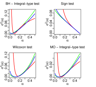
We consider the normal, the logistic and the Cauchy as null distributions. Using Theorem 3.3 we calculated the asymptotic variances of all our integral-type statistics, as well as the suprema of variance functions of the supremum-type statistics. In Figure 1 we present the limiting variances of some integral-type statistics as function of the trimming coefficient α𝛼\alpha. It can be noticed that for some values of α𝛼\alpha the variances are very close to each other. This ”asymptotic quasi distribution freeness” might be of practical importance providing an alternative to standard bootstrap procedures.
Refer to caption
Figure 1: Limiting variances of integral test statistics — green line – normal; blue line – logistic; red line – Cauchy;

For each null distribution, we consider two types of close alternatives from 𝒢𝒢\mathcal{G}:

  • a skew alternative in the sense of Fernandez-Steel [16], with the density

    g(x;θ)=21+θ+11+θ(g(x1+θ;0)I{x<0}+g((1+θ)x;0)I{x0})𝑔𝑥𝜃21𝜃11𝜃𝑔𝑥1𝜃0𝐼𝑥0𝑔1𝜃𝑥0𝐼𝑥0g(x;\theta)=\frac{2}{1+\theta+\frac{1}{1+\theta}}\Big{(}g(\frac{x}{1+\theta};0)I\{x<0\}+g((1+\theta)x;0)I\{x\geq 0\}\Big{)} (8)
  • a contamination alternative with the density

    g(x;θ)=(1θ)g(x;0)+θg(x1;0).𝑔𝑥𝜃1𝜃𝑔𝑥0𝜃𝑔𝑥10g(x;\theta)=(1-\theta)g(x;0)+\theta g(x-1;0). (9)

Another popular family of alternatives are the Azzalini skew alternatives (see [5]). However, in the case of the skew-normal distribution, all our test have zero efficiencies, while in the skew-Cauchy case, the Bahadur efficiency is not defined. Hence, these alternatives are not suitable for comparison, and we decided not to include them.

4.2 Bahadur equivalence

It turns out that some tests have identical Bahadur approximate slopes. With this in mind, we say that two tests are Bahadur equivalent if their Bahadur local approximate slopes coincide. It is then sufficient to consider just one representative from each equivalence class for comparison purposes.

We have the following Bahadur equivalence classes:

  • BHIMOI(1)NAI(2)NAI(3)similar-tosuperscriptBHIsuperscriptMOI1similar-tosuperscriptNAI2similar-tosuperscriptNAI3\rm BH^{I}\sim MO^{I}(1)\sim NA^{I}(2)\sim NA^{I}(3) for all 0α1/20𝛼120\leq\alpha\leq 1/2;

  • BHKMOK(1)NAK(2)NAK(3)similar-tosuperscriptBHKsuperscriptMOK1similar-tosuperscriptNAK2similar-tosuperscriptNAK3\rm BH^{K}\sim MO^{K}(1)\sim NA^{K}(2)\sim NA^{K}(3) for all 0α1/20𝛼120\leq\alpha\leq 1/2;

  • CMγMGGS(μ^(0))similar-toCM𝛾similar-toMGGsimilar-toS^𝜇0\rm CM\sim\gamma\sim MGG\sim S(\hat{\mu}(0));

  • KS(μ^(α))S(μ^(α))similar-toKS^𝜇𝛼S^𝜇𝛼\rm KS(\hat{\mu}(\alpha))\sim S(\hat{\mu}(\alpha)) (up to a certain value of α𝛼\alpha).

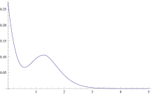
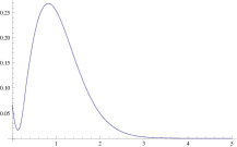
The first three equivalence classes can be easily obtained from the expressions for the corresponding Bahadur approximate slopes. For the fourth equivalence, notice that the term which is maximized in the KS statistic, for t=0𝑡0t=0, is twice the absolute value of the S statistic. So, these tests are equivalent whenever both the supremum of the asymptotic variance and the supremum of the limit in probability, are reached for t=0𝑡0t=0 (see Figure 2 as an example). This is the case for small α𝛼\alpha, from zero up to certain point that depends on the underlying null and alternative distributions.
Refer to caption
Refer to caption
Figure 2: Asymptotic variance functions σKS,F2(t)subscriptsuperscript𝜎2𝐾𝑆𝐹𝑡\sigma^{2}_{KS,F}(t) for α=0.1𝛼0.1\alpha=0.1 (left) and for α=0.4𝛼0.4\alpha=0.4 (right)

4.3 Discussion

Using Theorems 3.3-3.8 we calculated the local approximate Bahadur slopes for all statistics, all null and all alternative distributions.

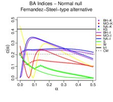
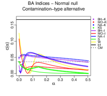
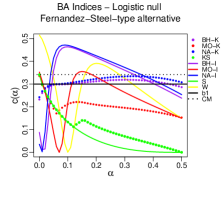
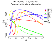
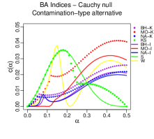
Taking into account the Bahadur equivalence, we choose the following tests: BHIsuperscriptBHI\rm BH^{I} and BHKsuperscriptBHK\rm BH^{K}; NAI(4)superscriptNAI4\rm NA^{I}(4) and NAK(4)superscriptNAK4\rm NA^{K}(4) (denoted as NAINAI\rm NA-I and NAKNAK\rm NA-K); MOI(2)superscriptMOI2\rm MO^{I}(2) and MOK(2)superscriptMOK2\rm MO^{K}(2) (denoted as MOIMOI\rm MO-I and MOKMOK\rm MO-K); S; W; and KS. For the convenience in presentation, we display the Bahadur approximate indices graphically as functions of α𝛼\alpha. We also present the indices of CMCM\rm CM and b1subscript𝑏1\sqrt{b_{1}} (denoted as b1b1\rm b1). Since they are not functions of α𝛼\alpha, we show them as horizontal lines.
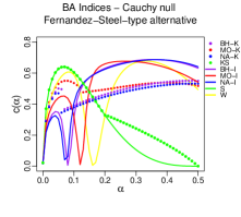
Refer to caption
Refer to caption
Figure 3: Comparison of Bahadur approximate indices – normal distribution
Refer to caption
Refer to caption
Figure 4: Comparison of Bahadur approximate indices – logistic distribution
Refer to caption
Refer to caption
Figure 5: Comparison of Bahadur approximate indices – Cauchy distribution

It is visible from all the figures that in the case of the integral-type statistics, the efficiencies vary significantly with α𝛼\alpha. In particular, for all the tests exist a value of α𝛼\alpha for which they have zero efficiencies. On the other hand, the supremum-type tests are much less sensitive to the change of α𝛼\alpha. The exception is the classical KS test which is by its definition inefficient for α=0.5𝛼0.5\alpha=0.5.

A natural way to compare tests, for a fixed null distribution, would be to compare the maximal values of their Bahadur indices over α[0,0.5]𝛼00.5\alpha\in[0,0.5]. It can be noticed that, in most cases, the integral-type tests outperform the supremum-type ones. The only exception is the contamination alternative to the Cauchy distribution. This is in concordance with the previous results (see e.g. [27, 31]).

In the case of normal distribution, the best of all tests are b1subscript𝑏1\sqrt{b_{1}}, and W for α=0𝛼0\alpha=0. In the case of the contamination alternative, MOI(2)superscriptMOI2\rm MO^{I}(2) test for α=0𝛼0\alpha=0 is also competitive. As far as the logistic distribution is concerned, NAI(4)superscriptNAI4\rm NA^{I}(4) and BHIsuperscriptBHI\rm BH^{I} are most efficient. In the case of the Cauchy null, the situation is different. The tests CM and b1subscript𝑏1\sqrt{b_{1}} are not applicable, and neither are the other tests for α=0𝛼0\alpha=0. Also, the “order” of the tests is much different for the two considered alternatives. In case of the Fernandez-Steel alternative, the best tests are MOI(2)superscriptMOI2\rm MO^{I}(2), NAI(4)𝑁superscript𝐴𝐼4NA^{I}(4) and BHIsuperscriptBHI\rm BH^{I}, while in the case of the contamination alternative, MOK(2)superscriptMOK2\rm MO^{K}(2) test is the most efficient.

As a conclusion, it is hard to recommend which test, and for which α𝛼\alpha, is the best to use in general, when the underlying distribution is completely unknown. The integral-type tests for small values of α𝛼\alpha could be the right choice, but they could also be calamities. In contrast, the supremum-type tests with α𝛼\alpha close or equal to 0.5 are quite reasonable, and, most importantly, never a bad choice.

Acknowledgement

We would like to thank the referees for their useful remarks. This work was supported by the MNTRS, Serbia under Grant No. 174012 (first author).

References

  • [1] I.A. Ahmad and Q. Li. Testing symmetry of an unknown density function by kernel method. J. Nonparametr. Stat., 7(3):279–293, 1997.
  • [2] M. Amiri and B.E. Khaledi. A new test for symmetry against right skewness. J. Stat. Comput. Simul., 86(8):1479–1496, 2016.
  • [3] A. Antille and G. Kersting. Tests for symmetry. Probab. Theory Related Fields, 39(3):235–255, 1977.
  • [4] A. Antille, G. Kersting, and W. Zucchini. Testing symmetry. J. Amer. Statist. Assoc., 77(379):639–646, 1982.
  • [5] A Azzalini. with the collaboration of A. Capitanio. The Skew-Normal and Related Families, Cambridge University Press, Cambridge, 2014.
  • [6] A. Baklizi. Testing symmetry using a trimmed longest run statistic. Aust. N. Z. J. Stat., 49(4):339–347, 2007.
  • [7] L. Baringhaus and N. Henze. A characterization of and new consistent tests for symmetry. Comm. Statist. Theory Methods, 21(6):1555–1566, 1992.
  • [8] L. Beghin and Ya. Yu. Nikitin. Approximate asymptotic Bahadur efficiency of independence tests with random sample size. Stat. Methods Appl., 8(1):1–23, 1999.
  • [9] P.K. Bhattacharya, J.L. Gastwirth, and A.L. Wright. Two modified Wilcoxon tests for symmetry about an unknown location parameter. Biometrika, 69(2):377–382, 1982.
  • [10] G. Burgio and Ya. Yu. Nikitin. The combination of the sign and Wilcoxon tests for symmetry and their Pitman efficiency. In Asymptotic Methods in Probability and Statistics with Applications, pages 395–407. Birkhäuser Boston, 2001.
  • [11] G. Burgio and Ya. Yu. Nikitin. On the combination of the sign and Maesono tests for simmetry and its efficiency. Statistica, 63(2):213–222, 2007.
  • [12] G. Burgio and S. Patrì. The most efficient linear combination of the sign and the Maesono tests for p-normal distributions. Statistica, 71(4):411, 2011.
  • [13] C.C. Butler. A test for symmetry using the sample distribution function. Ann. Math. Stat., 40(6):2209–2210, 1969.
  • [14] P. Cabilio and J. Massaro. A simple test of symmetry about an unknown median. Canad. J. Statist., 24(3):349–361, 1996.
  • [15] P.J. Farrell and K. Rogers-Stewart. Comprehensive study of tests for normality and symmetry: extending the Spiegelhalter test. J. Statist. Comput. Simul., 76(9):803–816, 2006.
  • [16] C. Fernandez and M. F. J. Steel. On Bayesian modeling of fat tails and skewness. J. Amer. Statist. Assoc., 93(441):359–371, 1998.
  • [17] J.L. Gastwirth. On the sign test for symmetry. J. Amer. Statist. Assoc., 66(336):821–823, 1971.
  • [18] R. Helmers, P. Janssen, and R. Serfling. Glivenko-Cantelli properties of some generalized empirical df’s and strong convergence of generalized L-statistics. Probab. Theory Related Fields, 79(1):75–93, 1988.
  • [19] N. Henze, Ya. Yu. Nikitin, and B. Ebner. Integral distribution-free statistics of Lp-type and their asymptotic comparison. Comput. Statist. Data Anal., 53(9):3426–3438, 2009.
  • [20] H.K. Iverson and R.H. Randles. The effects on convergence of substituting parameter estimates into U-statistics and other families of statistics. Probab. Theory Related Fields, 81(3):453–471, 1989.
  • [21] Michael R Kosorok. Introduction to empirical processes and semiparametric inference. Springer, 2008.
  • [22] V. V. Litvinova. New nonparametric test for symmetry and its asymptotic efficiency. Vestnik-St Petersburg University mathematics C/C of Vestnik-Sankt-Peterburgskii Univerzitet Matematika, 34(4):12–14, 2001.
  • [23] Y. Maesono. Competitors of the Wilcoxon signed rank test. Ann. Inst. Statist. Math., 39(1):363–375, 1987.
  • [24] M.B. Marcus and L.A. Shepp. Sample behavior of Gaussian processes. In Proc. of the Sixth Berkeley Symposium on Math. Statist. and Prob., volume 2, pages 423–441, 1972.
  • [25] S.G. Meintanis, Ya. Yu. Nikitin, and A.V. Tchirina. Testing exponentiality against a class of alternatives which includes the RNBUE distributions based on the empirical Laplace transform. J. Math. Sci. (N.Y.), 145(2):4871–4879, 2007.
  • [26] W. Miao, Y.R. Gel, and J.L. Gastwirth. A new test of symmetry about an unknown median. In Y. S. Chow and A. Chao, editors, Random Walk, Sequential Analysis and Related Topics–A Festschrift in Honor of Yuan-Shih Chow, pages 199–2014. Sigapore, World Scientific Pub, 2006.
  • [27] B. Milošević and M. Obradović. Characterization based symmetry tests and their asymptotic efficiencies. Statist. Probab. Lett., 119:155–162, 2016.
  • [28] B. Milošević and M. Obradović. New class of exponentiality tests based on U-empirical Laplace transform. Statist. Papers, 57(4):977–990, 2016.
  • [29] A. Mira. Distribution-free test for symmetry based on Bonferroni’s measure. J. Appl. Stat., 26(8):959–972, 1999.
  • [30] Ya. Yu. Nikitin. Large deviations of U-empirical Kolmogorov–Smirnov tests and their efficiency. J. Nonparametr. Stat., 22(5):649–668, 2010.
  • [31] Ya. Yu. Nikitin and M. Ahsanullah. New U-empirical tests of symmetry based on extremal order statistics, and their efficiencies. In M. Hallin, D. M. Mason, D. Pfeifer, and J. G. Steinebach, editors, Mathematical Statistics and Limit Theorems, Festschrift in Honour of Paul Deheuvels, pages 231–248. Springer International Publishing, 2015.
  • [32] Ya. Yu. Nikitin and I. Peaucelle. Efficiency and local optimality of nonparametric tests based on U- and V-statistics. Metron, LXII(2):185–200, 2004.
  • [33] R.H. Randles. On the asymptotic normality of statistics with estimated parameters. Ann. Statist., 10(2):462–474, 1982.
  • [34] E.D. Rothman and M. Woodroofe. A Cramér von-Mises type statistic for testing symmetry. Ann. Math. Stat., 43(6):2035–2038, 1972.
  • [35] R. J. Serfling. Approximation theorems of mathematical statistics. John Wiley & Sons, 1980.
  • [36] B.W. Silverman. Convergence of a class of empirical distribution functions of dependent random variables. Ann. Probab., 11(3):745–751, 1983.
  • [37] N. V. Smirnov. On the test of symmetry for the distribution of random variable. Dokl. Akad. Nauk SSSR, 56(1):13–16, 1947. (In Russian).
  • [38] T. Zheng and J.L. Gastwirth. On bootstrap tests of symmetry about an unknown median. J. Data Sci., 8(3):413, 2010.