Scalable Extended Dynamic Mode Decomposition using Random Kernel Approximation

Abstract

The Koopman operator is a linear, infinite-dimensional operator that governs the dynamics of system observables; Extended Dynamic Mode Decomposition (EDMD) is a data-driven method for approximating the Koopman operator using functions (features) of the system state snapshots. This paper investigates an approach to EDMD in which the features used provide random approximations to a particular kernel function. The objective of this is computational economy for large data sets: EDMD is generally ill-suited for problems with large state dimension, and its dual kernel formulation (KDMD) is well-suited for such problems only if the number of data snapshots is relatively small. We discuss two specific methods for generating features: random Fourier features, and the Nÿstrom method. The first method is a data-independent method for translation-invariant kernels only and involves random sampling in feature space; the second method is a data-dependent empirical method that may be used for any kernel and involves random sampling of data. We first discuss how these ideas may be applied in an EDMD context, as well as a means for adaptively adding random Fourier features. We demonstrate these methods on two example problems and conclude with an analysis of the relative benefits and drawbacks of each method.

1 Introduction

Dynamic Mode Decomposition (DMD) [37, 36, 40, 5] is a popular technique in model reduction for nonlinear dynamical systems. The goal of this method is to produce an approximation of the Koopman operator [35, 27, 26, 19] – a linear, infinite-dimensional operator that propagates system observables – using temporal snapshots of the system observables. As a linear operator, the Koopman operator may be completely described in terms of its eigenspectrum, and so the DMD process can be thought of as a data-driven method to approximate the leading eigenmodes, eigenvalues, and eigenfunctions. If the leading eigenfunctions of Koopman lie within the span of the observable state data used by DMD, then DMD can produce a good approximation of them. However, as pointed out in [42], DMD is only capable of producing an approximation of the eigenfunctions using linear monomials in the state. While this may be sufficient in cases where linear behavior dominates the dynamics, in many cases it is not, and so more sophisticated techniques must be used to approximate Koopman.

One such technique approaches this issue by generalizing the DMD machinery so that one is not limited to using system state data, but in fact may use functions (i.e., features) of the state data that may be more well-suited to approximating the Koopman eigenfunctions. This method is known as Extended DMD (EDMD) [42]. While certainly helpful in many contexts, EDMD is fundamentally a spectral method and hence suffers from the “curse of dimensionality”: the computational expense is dominated by the number of basis functions (features), which tends to grow quickly with increasing state dimension. This problem was partially solved by utilizing the so-called “kernel-trick”, which led to Kernel DMD (KDMD)[43], in which one need not explicitly transform the data into feature space; all that is required is knowledge of a kernel function that operates on the state data to produce inner products in feature space. However, while the computational expense of KDMD is not dominated by the number of basis functions, it is dominated by the number of snapshots and the state size. Hence, neither EDMD or KDMD are particularly well-suited to scenarios in which the state dimension and number of snapshots are both large.

The objective of this work is to make progress toward mitigating the computational expense of EDMD for scenarios in which the state size and number of snapshots are large. We propose doing this by using random features that generate efficient approximations to a particular kernel function. We will discuss this in greater detail later, but briefly, this choice is motivated by the theorems of Mercer and Bochner, which guarantee spectral decompositions of kernel functions under certain conditions. In choosing to use a random collection of features that approximate a particular kernel as the features in an EDMD method, we are conceptually producing a Monte Carlo approximation of the KDMD method, using EDMD. The intended advantage of this is, loosely, a blending of the best features of EDMD and KDMD: we wish to use the EDMD method so that we are not algorithmically limited by the number of snapshots, but also desire an efficent EDMD basis that does not scale as badly with state dimension as some of the more traditional feature choices (e.g., polynomial tensor products or radial basis functions (RBFs)). This claim is based on the hope that the chosen kernel function may be efficiently approximated with a modest number of features, and that therefore, the number of EDMD features required for a faithful Koopman approximation is modest as well. It is reasonable to expect that both the state size and complexity of the system dynamics could affect the rate of convergence of the EDMD algorithm; however, as we will see in the numerical examples, EDMD using kernel approximation methods can produce efficient, accurate Koopman approximations in benchmark problems with a state dimension large enough that most feature choices – like polynomials or RBFs – would be computationally intractable.

Depending on our choice of kernel, there are potentially two approaches for generating random features for EDMD: random Fourier features [31, 32], and the Nÿstrom method [41, 45]. In both methods, one begins by choosing a desired kernel function (which sets inner products in feature space). If the chosen kernel is positive semi-definite, symmetric, and translation-invariant, then Bochner’s theorem and the method of random Fourier features prescribes a representation in the Fourier basis, with the modes adhering to a distribution related to the kernel. In such a case, the EDMD features would consist of a finite collection of those modes, drawn randomly from their underlying distribution. If, instead, our kernel is not translation-invariant (but is positive semi-definite and symmetric), then Mercer’s theorem guarantees the existence of an eigendecomposition, which we may estimate empirically from data using the Nÿstrom method. In this more general case, the EDMD features would consist of the approximate kernel eigenfunctions.

To state the basic problem more concretely for background purposes, we assume we have access to a time-series of $(M+1)$ state snapshot vectors $\{x_{0},x_{1},\dots,x_{M}\}$, where any snapshot $x_{i}\in\mathbb{R}^{d}$. These data may have been generated by a nonlinear dynamical process, but DMD (and its variants) assumes that there is a corresponding linear dynamical system that can approximate those dynamics. In the case of DMD, this system is assumed linear in the state:

(1) $$Y=AX$$

where $X=\left[x_{0},x_{1},\dots,x_{M-1}\right]\in\mathbb{R}^{d\times M}$ and $Y=\left[x_{1},x_{2},\dots,x_{M}\right]\in\mathbb{R}^{d\times M}$ are the snapshot matrices and $A\in\mathbb{R}^{d\times d}$ is the DMD matrix. In the case of EDMD, following Williams [42], the system is assumed to be linear in some chosen feature space. That is, given a dictionary of $K$ functions acting on the state $\{\psi_{1}(x)\dots\psi_{K}(x)\}$, where $\psi_{i}(x):\mathbb{R}^{d}\mapsto\mathbb{R}$, we define the vector valued function $\Psi:\mathbb{R}^{d}\mapsto\mathbb{R}^{1\times K}$ as $\Psi(x)=\left[\psi_{1}(x)\dots\psi_{K}(x)\right]$ and assume the system dynamics are linear when written as:

(2) $$\Psi_{Y}=\Psi_{X}A$$

where $\Psi_{X},\Psi_{Y}\in\mathbb{R}^{M\times K}$ are the feature matrices, with row $j$ corresponding to $\Psi(x_{j})$, and $A\in\mathbb{R}^{K\times K}$ is the EDMD matrix. The EDMD Koopman matrix can thus be calculated as:

(3) $$A=\Psi_{X}^{\dagger}\Psi_{Y}$$

The computation of $A$ in Eq. 3 is easier by means of the equivalent formulation:

(4) $$A=G^{\dagger}H$$

where $G=\Psi_{X}^{T}\Psi_{X}$ and $H=\Psi_{X}^{T}\Psi_{Y}$. As $G,H\in\mathbb{R}^{K\times K}$, the cost of Eq. 4 is determined by $K$, and so the approaches we discuss in this paper – random Fourier features and the Nÿstrom approximation – are aimed at producing a good approximation to $A$ using an economical number $K$ of features.

To be clear – we are not attempting to improve the asymptotic scaling trends of EDMD with $K$, $M$, or $d$. Our goal is simply to apply a set of methods from machine learning in order to generate a basis which requires a relatively low value of $K$ for problems where both $d$ and $M$ are large.

We briefly pause here in order to step back and frame our work within a larger context. One of the reasons that Koopman analysis shows such promise in dynamical systems modeling is that it is a framework that can be approached in a purely data-driven manner, and data-driven learning is a paradigm that has enjoyed great progress recently. Indeed, advances in machine learning have demonstrated the power of empirically-trained models in a wide-range of computer science and applied mathematics applications, including computer vision [20, 38, 13], speech recognition [17, 7], manifold learning [6, 22, 29, 28], and stochastic process modeling [33, 23]. It is natural to hope to import the machinery underpinning these successes into the Koopman setting, and our work is a part of that effort.

Recent research has produced many computational approaches to approximating Koopman, including Generalized Laplace Analysis [4, 24, 25], the Ulam Galerkin Method [12, 2], and DMD. Of these, DMD is arguably the most popular, owing to its ease of implementation and the fact that it is well-suited to machine learning extensions (e.g., see [42, 43, 30]). While these properties make DMD a promising methodology, overwhelmingly large amounts of data can be problematic. For this reason, there is a community of researchers interested in developing scalable algorithms for data-driven tasks. In point of fact, a number of recent studies attempt to alleviate the computational burden of DMD, by leveraging the general concepts of randomization, compressive sampling, and/or sparsity; in particular, see [10, 11, 9, 3, 14, 18, 44, 16]. Of course, there are other aspects of DMD that require improvement besides scalability (see, for example, recent work in making DMD robust to noise [8, 15, 1]). Our present work fits within this general context and is hence part of a large communal push to develop scalable, efficient, robust data-driven algorithms for analysis of large dynamical systems.

We proceed as follows. First, we briefly review some background material on the basic theory of random Fourier features and the Nÿstrom method, and show how those ideas can be applied to EDMD. In the course of doing this, we also introduce some thoughts on how to adaptively and efficiently add more features in the random Fourier context in a way that makes use of previous calculations. We then apply both the random Fourier and Nÿstrom techniques to two example EDMD problems, and show how these methods provide an economical feature space for EDMD and hence an avenue for analyzing data which has large state size and number of snapshots. We conclude with an analysis of the computational runtime of the two methods, and a comparison of the relative benefits and drawbacks of each. We find that while the Nÿstrom method is the more general and accurate method, random Fourier features is the faster method for larger problems.

2 Random Fourier Features

We first describe the random Fourier feature method and how it may apply to EDMD. We begin with a brief review of the basic theory from the literature, and conclude with a proposition on how to adaptively add Fourier features in an EDMD problem efficiently.

2.1 Basis Selection

The main ideas we sketch here were first developed by Rahimi & Recht [31, 32]. Coined “Random Kitchen Sinks”, the method developed therein sought to expand a function in terms of a finite collection of random Fourier modes. The Fourier modes are chosen in that algorithm according to a pre-specified frequency distribution, which itself is derived from a pre-specified, translation-invariant kernel function. Viewed another way, Random Kitchen Sinks could be described as a method in which one first chooses a translation-invariant kernel function (which computes inner products in feature space), and then approximates that kernel function by means of Monte Carlo sampling a Fourier basis. This is possible by way of Bochner’s theorem.

Bochner’s theorem is the theoretical underpinning for the random Fourier feature method. Consider the kernel function $k(\cdot,\cdot):\mathbb{R}^{d}\times\mathbb{R}^{d}\mapsto\mathbb{R}$. It states that if that kernel function is positive semi-definite and translation-invariant (i.e., $k(x,x^{\prime})=k(x-x^{\prime})$), then it may be represented in a Fourier decomposition:

(5) $$k(x-x^{\prime})=\int_{z}\psi_{z}(x)\overline{\psi_{z}(x^{\prime})}\lambda(z)dz=\mathbb{E}_{z}\left[\psi_{z}(x)\overline{\psi_{z}(x^{\prime})}\right],$$

where $x,x^{\prime},z\in\mathbb{R}^{d}$, $\psi_{z}(x)=e^{i\langle z,x\rangle}$, and $\lambda(z)$ is a probability distribution associated with the kernel. The random Fourier feature method seeks to approximate this expectation with random sampling: a finite number $K$ of samples $\{z_{j}\}_{j=1}^{K}$ are drawn from the distribution $\lambda(z)$, and the sample average is calcuated:

(6) $$k(x-x^{\prime})\approx\frac{1}{K}\sum_{j=1}^{K}\psi_{z_{j}}(x)\overline{\psi_{z_{j}}(x^{\prime})}\;.$$

This approximation converges in expectation to the desired kernel; for more information about the rate of convergence or other details of the method, see [31, 32, 21].

The distribution $\lambda(z)$ may be found by taking the inverse Fourier transform of $k(x)$, from which we can see that $\lambda(z)$ that depends on the form of $k(x)$. For example, given a Gaussian kernel, the weights $\lambda(z)$ will also be normally-distributed in the frequency domain (but with the inverse covariance). Other choices of kernels (e.g., Laplacian, Cauchy) would lead to different corresponding forms of $\lambda(z)$.

The application we propose in the context of EDMD is to simply use this random Fourier basis as the EDMD features in Eq. 2.

2.2 Adaptive Feature Addition

One concern common to methods that approximate functions with a set of basis functions is adaptivity: if we compute a function surrogate with $K_{0}$ basis functions, and we wish to then add $K_{new}$ new basis functions, what is the least computationally burdensome method for doing this? In this section, we present a means for updating the Koopman operator using a group of new basis functions in a way that takes advantage of information from the previous computation and hence provides a modest computational advantage to recomputing everything from scratch. It should be noted that this method unfortunately does not help us calculate the Koopman eigenspectrum any more quickly; it is solely intended as a means to efficiently update the Koopman operator.

The motivation for this partially stems from recent work on streaming DMD [16]. In that context, however, the problem was to update the DMD Koopman approximation using sequentially obtained snapshots of data. Our problem is to update the EDMD Koopman approximation using a new group of basis functions (e.g., random Fourier modes), and hence the tactics used are different.

Let $K_{0}$ be the initial number of basis functions in Eq. 4. Given that we wish to update the matrices $\Psi_{X}$ and $\Psi_{Y}$ with new basis functions $\Psi_{X_{new}}$ and $\Psi_{Y_{new}}$, our goal is to update the matrices $G$, $H$, and $A$.

The first move we make is to simply note that since we have already calculated the inner products of each of the old basis functions with each other, we need not recalculate those terms in either $G$ or $H$. The updated matrix $G$ can be written as:

(7) $$G =\left[\begin{array}[]{c}\Psi_{X_{0}}^{T}\\ \hline\cr\Psi_{X_{new}}^{T}\end{array}\right]\left[\begin{array}[]{c|c}\Psi_{X_{0}}&\Psi_{X_{new}}\end{array}\right]$$

$$=\left[\begin{array}[]{c|c}\Psi_{X_{0}}^{T}\Psi_{X_{0}}&\Psi_{X_{0}}^{T}\Psi_{X_{new}}\\ \hline\cr\Psi_{X_{new}}^{T}\Psi_{X_{0}}&\Psi_{X_{new}}^{T}\Psi_{X_{new}}\end{array}\right]=\left[\begin{array}[]{c|c}G_{0}&G_{1}\\ \hline\cr G_{1}^{T}&G_{2}\end{array}\right]$$

The matrix $H$ has an analogous structure. Assuming we already have knowledge of $G_{0}$ from the previous EDMD calculation, only need calculate $G_{1}$ and $G_{2}$. The cost of calculating $G_{1}$ is $\mathcal{O}(K_{0}K_{new}M)$, and $G_{2}$ is $\mathcal{O}(K_{new}^{2}M)$. Arguments for the cost of updating $H$ are exactly parallel. Therefore, the cost of updating $G$ and $H$ is the greater of either $\mathcal{O}(K_{0}K_{new}M)$ or $\mathcal{O}(K_{new}^{2}M)$, depending on the relative sizes of $K_{0}$ or $K_{new}$, which denote the number of original and new basis functions, respectively.

The next step involved is to update $G^{\dagger}$. It is shown in [34] that if $G$ is a nonnegative, symmetric matrix with total rank equal to the sum of the ranks of $G_{0}$ and $G_{2}$, then the pseudoinverse may be calculated in block form as:

(8) $$G^{\dagger}=\left[\begin{array}[]{c|c}G_{0}^{\dagger}+G_{0}^{\dagger}G_{1}Q^{\dagger}G_{1}^{T}G_{0}^{\dagger}&-G_{0}^{\dagger}G_{1}Q^{\dagger}\\ \hline\cr-Q^{\dagger}G_{1}^{T}G_{0}^{\dagger}&Q^{\dagger}\end{array}\right]$$

where:

(9) $$Q=G_{2}-G_{1}^{T}G_{0}^{\dagger}G_{1}$$

Since $G$ is by definition a symmetric Gram matrix, a sufficient condition for satisfying the assumptions needed for Eq. 8 is that the basis functions be linearly independent. Furthermore, we already have knowledge of both $G_{0}$ and $G_{0}^{\dagger}$, which alleviates the cost of calculating Eq. 8. Therefore, the total cost of Eq. 8 is asymptotically dominated by the cost of the matrix products involving $G_{0}^{\dagger}$ and $G_{1}$, which is $\mathcal{O}(K_{0}^{2}K_{new})$. The last step involves forming the matrix product given in Eq. 4, which requires $\mathcal{O}((K_{0}+K_{new})^{3})$ time.

By comparison, explicit calculation from scratch of the updated matrices $G$ and $H$ would require $\mathcal{O}((K_{0}+K_{new})^{2}M)$ time; the pseudoinverse $G^{\dagger}$ would require $\mathcal{O}((K_{0}+K_{new})^{3})$ time; $G^{\dagger}H$ would require $\mathcal{O}((K_{0}+K_{new})^{3})$ time. Therefore, the computational savings obtained from using previous calculations would be largest when the number of new basis functions added is small relative to the number of original basis functions ($K_{new}\ll K_{0}$). Unfortunately, the final asymptotic scaling of calculating the Koopman matrix (Eq. 4) is the same regardless of the method used, but significant time could be saved in the calculation of $G$, $H$ and $G^{\dagger}$.

3 Nÿstrom Approximation

Thus far we have reviewed an approach to EDMD which could be described as deductive: we exploited the a-priori knowledge that translation-invariant kernels are well-approximated in the Fourier basis to generate an efficient basis for EDMD. This connection between a particular kernel and a corresponding basis is not always so clear, however, particularly if the assumption of translation-invariance does not hold. In light of this, one might wonder if there is a complementary inductive approach, whereby one need only specify the kernel function, and a basis for EDMD is then learned a-posteriori from some training data. The Nÿstrom method [41, 45] provides means for doing this.

The Nÿstrom method is a data-driven approach toward approximating the eigendecomposition of a kernel function. Here, we need not make the assumption of translation-invariance of the kernel; we only assume the kernel is symmetric and positive semi-definite. Under these less restrictive conditions, Bochner’s theorem no longer applies, but the more general Mercer’s theorem does. Mercer’s theorem guarantees us that any such kernel function $k(\cdot,\cdot):\mathbb{R}^{d}\times\mathbb{R}^{d}\mapsto\mathbb{R}$ may be expanded in terms of the following infinite summation:

(10) $$k(x,y)=\sum_{j=1}^{\infty}\lambda_{j}\psi_{j}(x)\psi_{j}(y)\;,$$

where $\{\lambda_{j},\psi_{j}(x)\}$ are eigenvalues/functions of the Hilbert-Schmidt integral operator that is associated with the kernel:

(11) $$T_{k}\left(\psi_{j}(y)\right)=\int_{x}k(y,x)\psi_{j}(x)p(x)dx=\mu_{j}\psi_{j}(y)\;.$$

Here, $p(x)$ denotes the probability density function of the data $x$. The Nÿstrom method seeks to construct a Monte Carlo approximation to the integral in Eq. 11 using a finite sample of data $\{x_{1}\dots x_{K}\}$ drawn from $p(x)$:

(12) $$\frac{1}{K}\sum_{j}^{K}k(y,x_{j})\psi_{i}(x_{j})\approx\lambda_{i}\psi_{i}(y)\;.$$

When this equation is written for each of the $K$ data points, we produce the following matrix eigenproblem:

(13) $$M_{k}U=U\Lambda$$

where $M_{k},U,\Lambda\in\mathbb{R}^{K\times K}$, $(M_{k})_{i,j}=k(x_{i},x_{j})$. Approximations of the kernel eigenvalues and eigenfunctions at the $K$ data points are then:

(14) $$\psi_{i}(x_{j})\approx\sqrt{K}U_{j,i}\;\;\;,\;\;\;\lambda_{i}\approx\frac{\Lambda_{i,i}}{K}$$

Furthermore, approximations at another data point $y$ may be interpolated:

(15) $$\psi_{i}(y)\approx\frac{\sqrt{K}}{\Lambda_{i,i}}\sum_{j}^{K}k(y,x_{j})U_{j,i}$$

To proceed for EDMD purposes, we must produce the feature matrices $\Psi_{X}$ and $\Psi_{Y}$ in Eq. 3. At this point, we have a choice. One option is to make use of the entire dataset and use Eq. 15 to interpolate $\Psi_{X}$ at the remaining $\left(M-K\right)$ points and $\Psi_{Y}$ at all $M$ data points. A second, cheaper option is to simply use the evaluation Eq. 14 on the $K$ points that we already have as $\Psi_{X}$, and only interpolate $\Psi_{Y}$ on those $K$ points using Eq. 15. In what follows, the former method will be referred to as the “expensive” Nÿstrom variant; the latter will be referred to as the “cheap” variant. Of course, one may also elect to use an interpolation on some arbitrary subset of the data between those two extremes. The choice is up to the user, although – as we will see – it can have predictable consequences in terms of the speed/accuracy trade-off.

Notice that this Nÿstrom method is more general than the random Fourier feature method, as nowhere have we been required to assume that the kernel function is translation-invariant. Although the Nÿstrom features are not theoretically exact as was the case in the random Fourier feature method, they are derived from the data we collect, which gives them a direct connection to the problem at hand that may provide some compensating benefit.

4 Numerical Examples

We now present two numerical experiments that give some empirical evidence demonstrating the efficacy of EDMD using either random Fourier features or the Nÿstrom method.

Before proceeding, the topic of kernel selection – which is central to both of these approaches – should be discussed. Clearly, the choice of a kernel can have a large effect on the efficiency and/or accuracy of the results. The approach that we follow in this paper is to use the data we have to estimate an acceptable kernel. We calculate Euclidean distances between snapshots, and use the resulting statistics to estimate the standard deviation of a Gaussian distribution. It should be acknowledged up front that this is a bit of a heuristic that may be unsatisfying to those who would want a more rigorous approach. However, we were able to obtain satisfactory results in the following examples with this. If a more rigorous approach is desired, it may be possible to choose a kernel form (e.g., Gaussian), and then tune the shape parameter of that distribution with cross-validation. One might even extend this cross-validation to include multiple kernel forms (e.g., Laplacian, Cauchy) with various shape parameters. It would be interesting to perform a follow-up study to investigate whether an approach like this could yield improved results; however, in order not to detract from the central narrative of this paper, we do not pursue that discussion here any further.

4.1 Fitzhugh-Nagumo Equations

Here, following Williams [43], we examine the 1-D Fitzhugh-Nagumo equations as a test case. This example is attractive for several reasons. First, it provides a problem with a moderately-sized state dimension, which makes it challenging for the more traditional basis choices in EDMD (at least, without the pre-application of some form of data compression, such as POD). Second, the leading two Koopman modes can be deduced from the system linearization and, hence, regular DMD can produce them for comparison purposes.

The equations read thus:

(16) $$v_{t} =v_{xx}+v-w-v^{3}$$

$$w_{t} =w_{xx}+\epsilon(v-c_{1}w-c_{0})$$

on the domain $x\in[0,20]$ and with the parameter values $c_{0}=-0.03$, $c_{1}=2.0$, $\delta=4.0$, $\epsilon=0.02$. The boundary conditions used are Neumann, and we solve these equations using a simple structured grid of 100 spatial points. Our goal is to extract the Koopman modes for $v$, and so our state dimension $d=100$. We use 2500 snapshot pairs, taken at temporal intervals of $\Delta t=1$. The initial conditions used are the standing wave fronts in $v$ and $w$, and the system is perturbed every $25\Delta t$ by a simple Gaussian process.

Fig. 1 shows computations of the leading Koopman eigenvalues and modes using a random Fourier basis with Monte Carlo sample sizes ranging from 100 to 1000. Fig. 2 shows the equivalent computations using the expensive Nÿstrom method with random snapshot sample sizes ranging from 100 to 1000. The random Fourier basis frequencies are normally-distributed with a standard deviation of $\sigma=4\pi$ (corresponding to a normally-distributed kernel function with the inverse standard deviation); the kernel function used in the Nÿstrom method is a Gaussian with $\sigma=1$. In both cases, we determine the shape parameter $\sigma$ empirically from the data set: we calculate distances between data snapshots and estimate an average distance between them.

In the random Fourier feature results, the two leading (linear) Koopman modes converge relatively quickly and strongly to the correct answer (as judged by regular DMD), requiring around 500-600 basis functions to accurately represent. The corresponding Koopman eigenvalues converge quickly as well. The next two (nonlinear) Koopman modes present, predictably, more variance in shape with number of basis functions, and require more basis functions (around 900) to converge. Similarly, there is more variation in the calculated Koopman eigenvalues that correspond to those two nonlinear Koopman modes.

It appears Koopman modes computed with the expensive Nÿstrom method may be converging sooner than those computed with random Fourier features. The most noticeable difference demonstrating this is the shape of the modes using lower numbers of snapshots. In the Fourier approach, around 500-600 basis functions were required before the modes began to qualitatively resemble the correct answers; in the Nÿstrom approach, qualitative correctness is achieved almost instantly at 100 snapshots.

It should be clear, however, that both methods provide fairly good approximations of the leading Koopman modes/eigenvalues in this problem, with only 1000 random samples or less. This is a reasonable number of basis functions for a state dimension of $d=100$, compared to the more traditional basis choices.

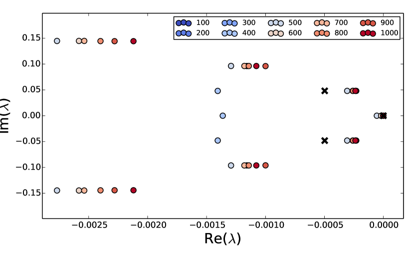
(a) Eigenvalues (DMD eigenvalues displayed as black $\times$ markers).

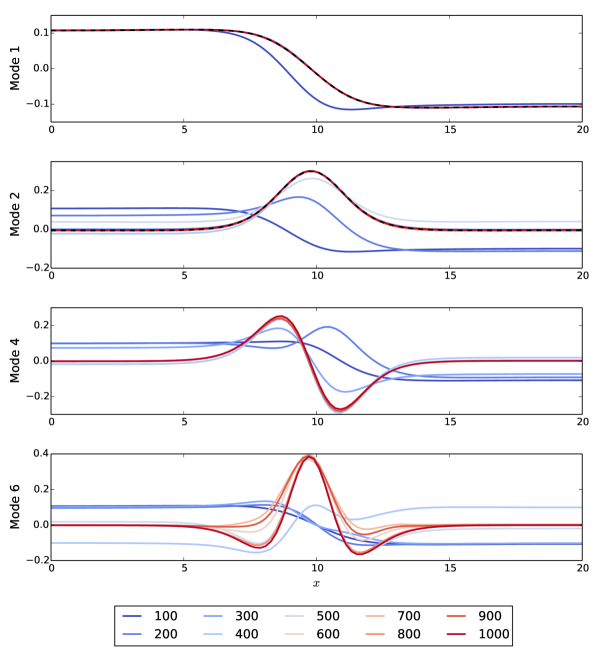
(b) Modes (DMD modes displayed as dashed black lines).

Figure 1: Fitzhugh-Nagumo eigenvalues and modes, using DMD and random Fourier EDMD with varying numbers of basis functions.

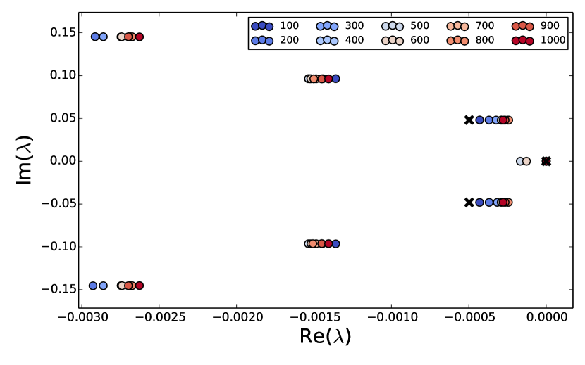
(a) Eigenvalues (DMD eigenvalues displayed as black $\times$ markers).

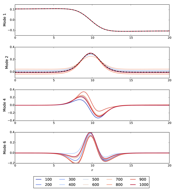
(b) Modes (DMD modes displayed as dashed black lines).

Figure 2: Fitzhugh-Nagumo eigenvalues and modes, using DMD and the “expensive” Nÿstrom method EDMD with varying numbers of basis functions.

4.2 Experimental Cylinder Flow Data

Our final demonstration involves a data set in which both the state dimension and the number of snapshots are both quite large. We analyze PIV data of 2D cylinder flow [39], consisting of a $80\times 135$ Cartesian grid of spatial points ($d=10,800$) sampled at $M=8,000$ snapshots in time. This data set has been analyzed previously using DMD [39], KDMD [43], and streaming DMD [16]; the interested reader is encouraged to consult those references for more information on this data set.

As both $d$ and $M$ are approximately $10^{4}$, both regular DMD and EDMD (with traditional basis choices) are either impractical or impossible for the full data set: DMD can be performed on this data set (see [39]), but that requires several cores running in parallel and is extremely computationally expensive; EDMD based on tensor polynomials or RBFs clearly suffers from the large state dimensionality. KDMD necessitates the SVD computation of a $M\times M$ matrix ($\mathcal{O}(M^{3})$ computational scaling) and hence is expensive as well; because of this expense, it is only performed on a subset of the full data in [43]. Of course, it may be argued that a pre-processing data compression step (e.g., POD) could be applied to make the problem more computationally tractable by reducing the effective state dimension. While that could be a feasible approach, we are interested in addressing situations where the state dimension (and number of snapshots) is large (which might be the case even after any data pre-processing, depending on the problem). Therefore, as in the previous example, we do not apply any such dimension-reduction pre-processing.

This data set is well-suited for analysis using either random Fourier EDMD or the Nÿstrom method. As in the previous example, we select the Fourier modal frequencies from a normal distribution, which effectively approximates a Gaussian kernel with the inverse variance. The Fourier modal distribution variance is, as before, determined empirically from the data set (we use $\sigma=1/400$). In the Nÿstrom approach, we use a Gaussian kernel function with the inverse shape parameter used in the random Fourier method (i.e., the Nÿstrom kernel is a Gaussian with $\sigma=400$). We test both the “expensive” version of the Nÿstrom method, in which we interpolate the feature matrices $\Psi_{X}$ and $\Psi_{Y}$ on all $M$ data points, and the “cheap” version, in which we only interpolate $\Psi_{Y}$ on the $K$ random sample data points.

Fig. 3 displays the leading Koopman modes and eigenvalues, computed with the random Fourier method, for $K=100,\;200,\;500$, and $1000$. Figs. 4 and 5 show equivalent computations using the cheap and expensive Nÿstrom variants (respectively) with identical numbers $K$ of features. Using the Fourier method, we see good convergence of the first four Koopman modes when using around $500$ to $1000$ Fourier modes; this is remarkable given both the large state and snapshot sizes of the data set. Certainly – as before – the higher order modes require more basis functions to converge (e.g., the first mode converges well using $K<100$, while the fourth Koopman mode requires 500 to 1000 basis functions), but this asymetry in modal resolution is found in EDMD/KDMD as well and so does not represent a weakness unique to Fourier EDMD. We should also note that the Fourier EDMD method (as well as the Nÿstrom method) retains an advantage of EDMD/KDMD in that the leading Koopman modes may be determined by the proximity of their eigenvalues to the imaginary axis (as opposed to the “cloud” of eigenvalues produced in DMD in which the dominant modes must be determined using energy-based or sparsity-promoting methods).

In comparison, it appears yet again that convergence is relatively faster using the expensive Nÿstrom variant, with respect to both the eigenvalues and eigenvectors. In particular, the fourth Koopman mode is qualitatively well approximated in the expensive Nÿstrom method using only 100 empirical eigenfunction features, while 100 random Fourier features is not sufficient for this purpose. However, accuracy using the cheap Nÿstrom variant is more or less equal to that using random Fourier features.

In all methods, it does appear that convergence is slowest for the real parts of the Koopman eigenvalues – the four modes should all have eigenvalues lying on the imaginary axis. While the imaginary components are in good agreement with the reported values in previous studies, the real components are noticeably larger in magnitude than they should be (although this magnitude clearly decreases with increasing $K$). One consequence of this is a “bowing” of the eigenvalues, which is a common observation in EDMD/KDMD. Regardless of this, we clearly see the utility of the two approaches on display in this example: we are able to extract good approximations of the leading components of the Koopman spectrum using only around 1000 EDMD features, which is in stark contrast to the time and resources required to do the same using DMD, KDMD, or EDMD (with traditional basis choices).

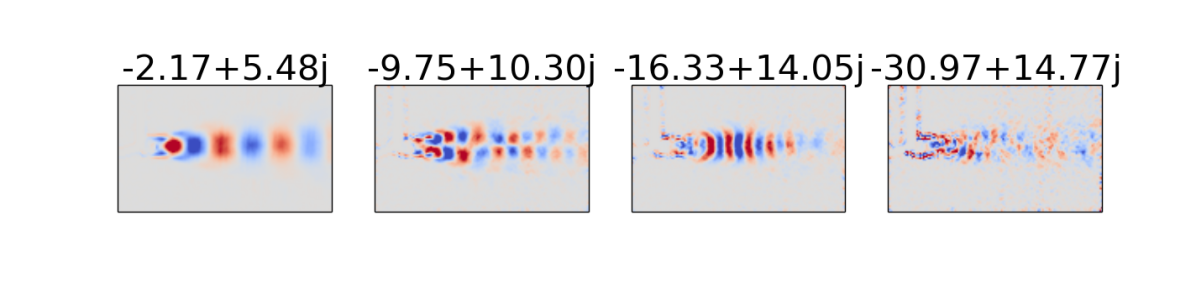
(a) $K=100$

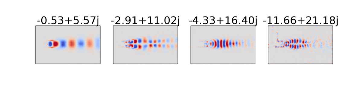
(b) $K=500$

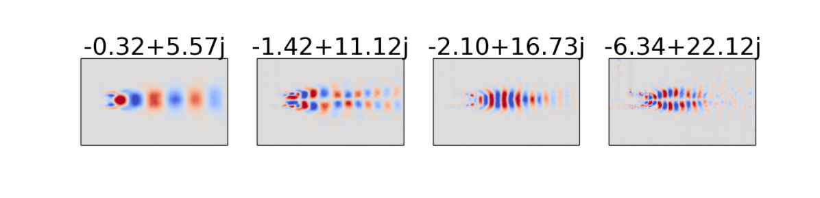
(c) $K=1000$

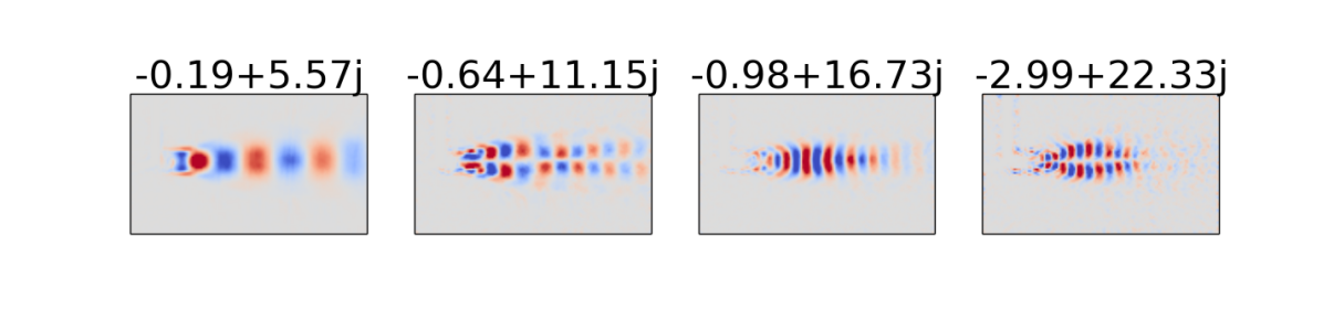
(d) $K=2000$

Figure 3: Leading Koopman mode and eigenvalue approximations for the cylinder PIV data, using random Fourier EDMD with varying numbers of basis functions ($K$).

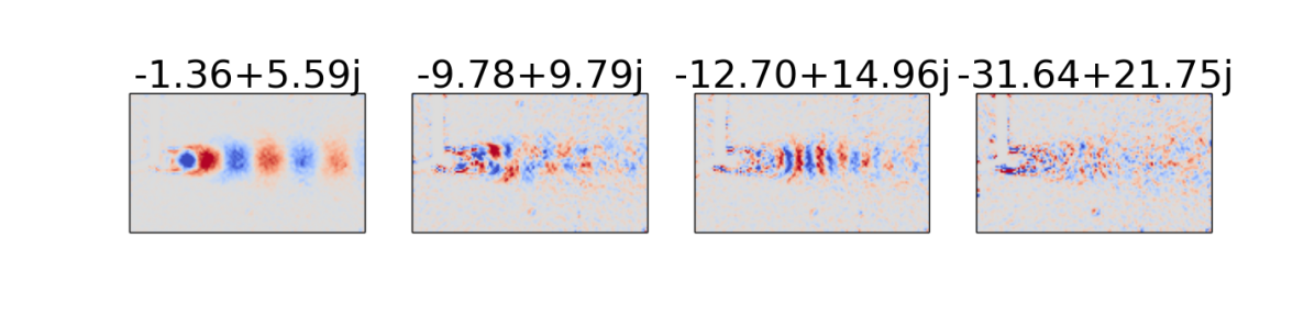
(a) $K=100$

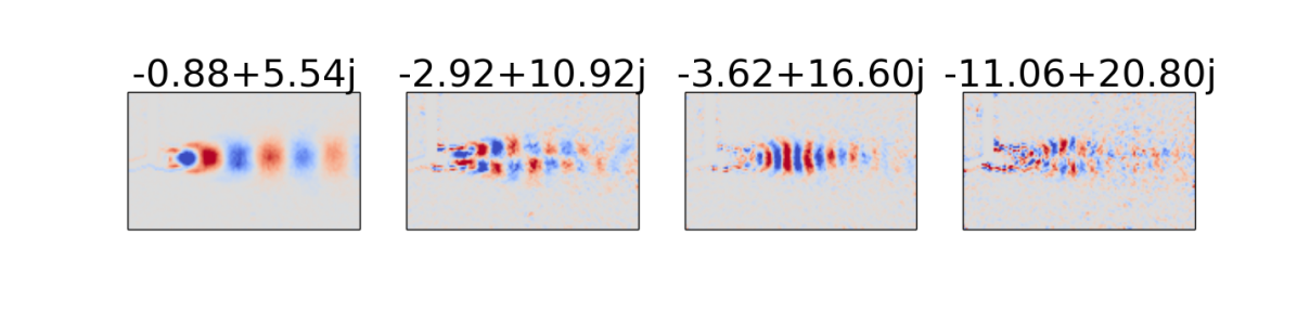
(b) $K=500$

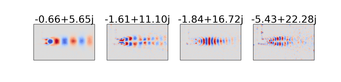
(c) $K=1000$

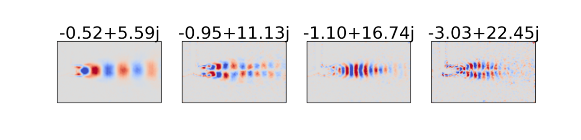
(d) $K=2000$

Figure 4: Leading Koopman mode and eigenvalue approximations for the cylinder PIV data, using the “cheap” Nÿstrom method EDMD with varying numbers of basis functions ($K$).

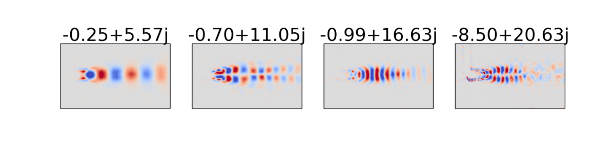
(a) $K=100$

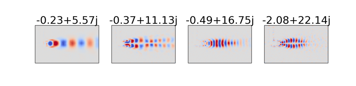
(b) $K=500$

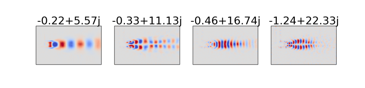
(c) $K=1000$

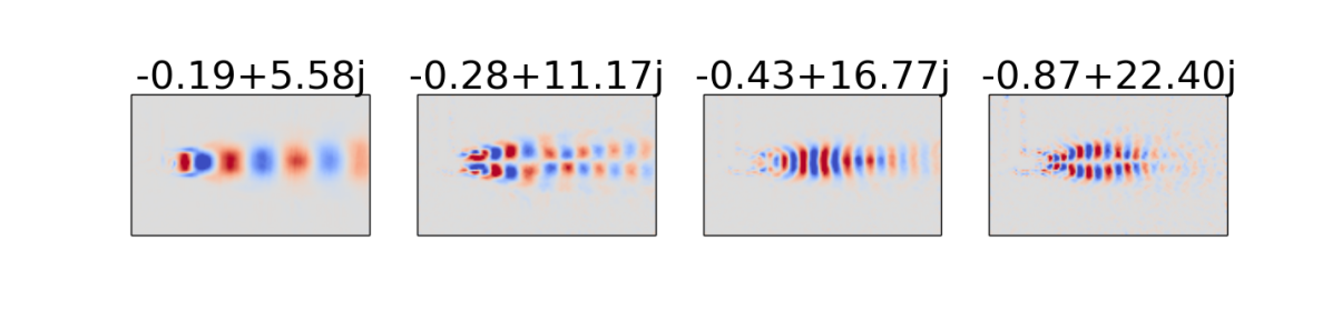
(d) $K=2000$

Figure 5: Leading Koopman mode and eigenvalue approximations for the cylinder PIV data, using the “expensive” Nÿstrom method EDMD with varying numbers of basis functions ($K$).

4.3 Computational Scaling

Computationally speaking, there are some differences between the random Fourier, cheap Nÿstrom, and expensive Nÿstrom methods. The first difference involved is in how the basis elements are computed. Basis computation in the Nÿstrom method occurs in two distinct steps. The first is to compute the empirical eigenfunctions at the $K$ random data points. This involves computing the kernel matrix for the $K$ random sample points ($\mathcal{O}(\frac{1}{2}K^{2}d)$) and then computing the eigendecomposition of that $K\times K$ kernel matrix ($\mathcal{O}(K^{3})$). The second is to interpolate those eigenfunctions. In the expensive Nÿstrom variant, this interpolation occurs for $\Psi_{X}$ and $\Psi_{Y}$ at all $M$ data points (Eq. 15), which involves computing two $M\times K$ kernel matrices ($\mathcal{O}(MKd)$) and multiplying each of them with a $K\times K$ matrix ($\mathcal{O}(2MK^{2})$). Thus, the total runtime for the expensive Nÿstrom basis computation scales asymptotically as $\mathcal{O}(KMd+K^{2}(d+M)+K^{3})$. In the cheap Nÿstrom variant, eigenfunction interpolation only occurs for $\Psi_{Y}$ at the $K$ random data points, which involves computing a $K\times K$ kernel matrix ($\mathcal{O}(\frac{1}{2}K^{2}d)$) and multiplying it with a $K\times K$ matrix ($\mathcal{O}(K^{3})$). Thus, the asymptotic scaling for the cheap Nÿstrom variant is $\mathcal{O}(K^{2}d+K^{3})$. In random Fourier EDMD, the random Fourier basis must simply be calculated at all data points, which is $\mathcal{O}(KMd)$. Thus, we see that the random Fourier method will always be faster than the expensive Nÿstrom method for basis generation; how the random Fourier method compares to the cheap Nÿstrom method will generally depend on the parameter values.

The remaining two steps involved in EDMD are the calculation of the Koopman matrix and its eigendecomposition (for details, see [42]). The Koopman operator calculation scales as $\mathcal{O}(K^{2}M+K^{3})$. The eigendecomposition calculation scales as $\mathcal{O}(KMd+K^{2}d+K^{3})$ for the random Fourier and expensive Nÿstrom methods and $\mathcal{O}(K^{2}d+K^{3})$ for the cheap Nÿstrom method. These asymptotic scalings are summarized in Table 1. Note that in this table, “CN” denotes the cheap Nÿstrom method, “RF” the random Fourier method, and “EN” the expensive Nÿstrom method.

Table 1: Asymptotic Computational Scalings

	Basis	Koopman	Eigenspectrum
CN	$K^{2}d+K^{3}$	$K^{3}$	$K^{2}d+K^{3}$
RF	$KMd$	$K^{2}M+K^{3}$	$KMd+K^{2}d+K^{3}$
EN	$KMd+K^{2}(d+M)+K^{3}$	$K^{2}M+K^{3}$	$KMd+K^{2}d+K^{3}$

To illustrate concretely by way of examples, Fig. 6 presents runtimes for the random Fourier and Nÿstrom methods using problems with increasing values of $K$, $M$, and $d$, broken down by each of the steps in the process (basis computation, Koopman matrix calculation, and Koopman eigendecomposition). The three tests displayed in that figure were chosen to investigate runtimes in the regime where $K\ll d,M$, since that is the regime in which these methods are intended to be used. The total runtimes of both the random Fourier and expensive Nÿstrom methods remain relatively constant for each of the tests, while that of the cheap Nÿstrom method increases linearly with increasing $d$. This is the expected behavior on the basis of Table 1: the product $KMd$ is the dominant term in the scaling laws for the random Fourier and expensive Nÿstrom methods, and it is constant throughout each of the tests. Conversely, the cheap Nÿstrom method does not scale with $KMd$; the linear upward trend visible is a result of the $K^{2}d$ term in both the basis and eigendecomposition calculations. We also see clear confirmation that the expensive Nÿstrom method generally has the longest total runtime of all the methods, a consequence of the high cost of basis computation. While the cheap Nÿstrom method is less expensive than the random Fourier method in these three examples, it is important to note that we cannot in general conclude that it will always be faster. We can make the general observation that the cheap Nÿstrom method will be the fastest when $d\ll M$ (i.e., lower state dimension, higher number of snapshots), since the random Fourier and expensive Nÿstrom methods scale linearly with $M$ but the cheap Nÿstrom method is independent of $M$ (a nice feature).

Incorporating this information yields a complex set of relative benefits and drawbacks when comparing the methods. Our numerical experiments seem to indicate that the expensive Nÿstrom method is more accurate than the other methods, given the same values of $K,M,d$. Both of the Nÿstrom methods are more flexible, in the sense that they can approximate a wider class of kernels, and they have a closer relationship to the data. Additionally, the cheap Nÿstrom method does not scale with $M$, since it only uses a random subsampling of the full data set to generate the empirical basis. However, the random Fourier method uses eigenfunctions that are more mathematically precise for translation-invariant kernels than the data-approximated ones generated by Nÿstrom. Additionally, we have a method for efficiently adding random Fourier features (§ 2.2), which is another speed-based attractive feature.

Lastly, some comments on how these methods compare to “regular” EDMD/KDMD are in order. It is important here to recall the overall objective of this paper: our goal was not to improve the asymptotic computational scaling of EDMD with respect to the parameters $K,M,d$; rather, it was to develop and use highly efficient EDMD basis functions that effectively make the value of $K$ much less than what it otherwise would be using traditional basis choices for problems with large $d,M$. Hence, although the computational scaling for regular EDMD is essentially the same as it is for the Nÿstrom and random Fourier methods, both the Nÿstrom and random Fourier methods are able to handle problems that would require an infeasibly large number of basis functions if approached with regular EDMD. Similar arguments exist regarding KDMD, as its runtime is dominated by $M^{3}$.

Figure 6: Computational runtimes. Parameters used in the five tests are: $d=\{10^{3},10^{4},10^{5}\}$, $M=\{10^{5},10^{4},10^{3}\}$, $K=\{10^{2},10^{2},10^{2}\}$, respectively. Bar color divisions are linear percentages of the total respective computational runtimes (given as the total bar heights).

5 Conclusions

The objective of this work was to make progress toward reducing the computational demands of EDMD/KDMD for data sets with large state and snapshot sizes. To do this, we imported ideas from the theory of random approximations of kernel functions, and used these ideas to give us an economical set of EDMD features. We presented two numerical examples which demonstrate how we can obtain good approximations of the Koopman modes/eigenvalues for problems with large state and snapshot sizes using a very reasonable number of basis functions.

We observed a complex set of trade-offs involved in comparing the random Fourier and Nÿstrom methods. We saw that the expensive Nÿstrom method generally provides higher accuracy, but at an increased computational cost, for the same values of $K$, $M$, and $d$. The cheap Nÿstrom method computational runtime does not scale with $M$. The Nÿstrom methods are more flexible in the sense that they can represent a wider range of kernels, while the random Fourier method is more flexible in the sense that features can be added adaptively.

One avenue that may be of future research interest involves speeding up the random Fourier basis computation. It has already been shown in [21] that Hadamard transforms may be used to obtain fast approximations to the random Fourier basis computation; however, the method as it stands computes a number of basis functions that is equal to or greater than the state dimension, which might cancel its economical gains when $K\ll d$ (as is the case in many problems of interest).

6 Acknowledgments

Los Alamos Report LA-UR-17-29880. Funded by the Department of Energy at Los Alamos National Laboratory under contract DE-AC52-06NA25396. The authors also wish to acknowledge Scott Dawson for helpful technical feedback and Mark Lohry for helpful advice on visually displaying data.

References

- [1] S. Bagheri, Effects of weak noise on oscillating flows: linking quality factor, floquet modes, and koopman spectrum, Physics of Fluids, 26 (2014), p. 094104.
- [2] E. M. Bollt and N. Santitissadeekorn, Applied and Computational Measurable Dynamics, vol. 18, SIAM, 2013.
- [3] S. L. Brunton, J. L. Proctor, J. H. Tu, and J. N. Kutz, Compressive sampling and dynamic mode decomposition, Journal of Computational Dynamics, 2 (2018), pp. 165–191.
- [4] M. Budišić, R. Mohr, and I. Mezić, Applied koopmanism, Chaos: An Interdisciplinary Journal of Nonlinear Science, 22 (2012), p. 047510.
- [5] K. K. Chen, J. H. Tu, and C. W. Rowley, Variants of dynamic mode decomposition: boundary condition, koopman, and fourier analyses, Journal of Nonlinear Science, 22 (2012), pp. 887–915.
- [6] R. R. Coifman and S. Lafon, Diffusion maps, Applied and Computational Harmonic Analysis, 21 (2006), pp. 5–30.
- [7] G. E. Dahl, D. Yu, L. Deng, and A. Acero, Context-dependent pre-trained deep neural networks for large-vocabulary speech recognition, IEEE Transactions on audio, speech, and language processing, 20 (2012), pp. 30–42.
- [8] S. T. Dawson, M. S. Hemati, M. O. Williams, and C. W. Rowley, Characterizing and correcting for the effect of sensor noise in the dynamic mode decomposition, Experiments in Fluids, 57 (2016).
- [9] N. B. Erichson, S. L. Brunton, and J. N. Kutz, Compressed dynamic mode decomposition for background modeling, Journal of Real-Time Image Processing, (2016), pp. 1–14.
- [10] N. B. Erichson, S. L. Brunton, and J. N. Kutz, Randomized dynamic mode decomposition. arXiv:1702.02912, 2017.
- [11] N. B. Erichson and C. Donovan, Randomized low-rank dynamic mode decomposition for motion detection, Computer Vision and Image Understanding, 146 (2016), pp. 40–50.
- [12] G. Froyland, G. A. Gottwald, and A. Hammerlindl, A computational method to extract macroscopic variables and their dynamics in multiscale systems, SIAM Journal on Applied Dynamical Systems, 13 (2014), pp. 1816–1846.
- [13] R. Girshick, J. Donahue, T. Darrell, and J. Malik, Rich feature hierarchies for accurate object detection and semantic segmentation, in Proceedings of the IEEE Conference on Computer Vision and Pattern Recognition, 2014, pp. 580–587.
- [14] F. Guéniat, L. Mathelin, and L. R. Pastur, A dynamic mode decomposition approach for large and arbitrarily sampled systems, Physics of Fluids, 27 (2015), p. 025113.
- [15] M. S. Hemati, C. W. Rowley, E. A. Deem, and L. N. Cattafesta, De-biasing the dynamic mode decomposition for applied koopman spectral analysis of noisy datasets, Theoretical and Computational Fluid Dynamics, 31 (2017), pp. 349–368.
- [16] M. S. Hemati, M. O. Williams, and C. W. Rowley, Dynamic mode decomposition for large and streaming datasets, Physics of Fluids, 26 (2014).
- [17] G. Hinton, L. Deng, D. Yu, G. E. Dahl, A. Mohamed, N. Jaitly, A. Senior, V. Vanhoucke, P. Nguyen, T. N. Sainath, and B. Kingsbury, Deep neural networks for acoustic modeling in speech recognition: The shared views of four research groups, IEEE Signal Processing Magazine, 29 (2012), pp. 82–97.
- [18] M. R. Jovanović, P. J. Schmid, and J. W. Nichols, Sparsity-promoting dynamic mode decomposition, Physics of Fluids, 26 (2014), p. 024103.
- [19] B. O. Koopman, Hamiltonian systems and transformation in hilbert space, Proceedings of the National Academy of Sciences, 17 (1931), pp. 315–318.
- [20] A. Krizhevsky, I. Sutskever, and G. E. Hinton, Imagenet classification with deep convolutional neural networks, Advances in Neural Information Processing Systems, (2012), pp. 1097–1105.
- [21] Q. Le, T. Sarlos, and A. Smola, Fastfood – approximating kernel expansions in loglinear time, in Proceedings of the international conference on machine learning, JMLR: W&CP volume 28, 2013.
- [22] J. A. Lee and M. Verleysen, Nonlinear dimensionality reduction, Springer, 2007.
- [23] D. J. MacKay, Introduction to gaussian processes, NATO ASI Series F Computer and Systems Sciences, 168 (1998), pp. 133–166.
- [24] A. Mauroy and I. Mezić, On the use of Fourier averages to compute the global isochrons of (quasi) periodic dynamics, Chaos: An Interdisciplinary Journal of Nonlinear Science, 22 (2012), p. 033112.
- [25] A. Mauroy, I. Mezić, and J. Moehlis, Isostables, isochrons, and koopman spectrum for the action-angle representation of stable fixed point dynamics, Physica D: Nonlinear Phenomena, 261 (2013), pp. 19–30.
- [26] I. Mezić, Spectral properties of dynamical systems, model reduction and decompositions, Nonlinear Dynamics, 41 (2005), pp. 309–325.
- [27] I. Mezić, Analysis of fluid flows via spectral properties of the koopman operator, Annual Review of Fluid Mechanics, 45 (2013), pp. 357–378.
- [28] B. Nadler, S. Lafon, R. R. Coifman, and I. G. Kevrekidis, Diffusion maps, spectral clustering and eigenfunctions of fokker-planck operators, in NIPS, 2005.
- [29] B. Nadler, S. Lafon, R. R. Coifman, and I. G. Kevrekidis, Diffusion maps, spectral clustering and reaction coordinates of dynamical systems, Applied and Computational Harmonic Analysis, 21 (2006), pp. 113–127.
- [30] S. E. Otto and C. W. Rowley, Linearly-recurrent autoencoder networks for learning dynamics. arXiv:1712.01378, 2017.
- [31] A. Rahimi and B. Recht, Random features for large-scale kernel machines. NIPS 20, 2007.
- [32] A. Rahimi and B. Recht, Weighted sums of random kitchen sinks: replacing minimization with randomization in learning. NIPS 21, 2008.
- [33] C. E. Rasmussen, Gaussian processes in machine learning, in Advanced lectures on machine learning, Springer, 2004, pp. 63–71.
- [34] C. A. Rohde, Generalized inverses of partitioned matrices, J. Soc. Indust. Appl. Math., 13 (1965), pp. 1033–35.
- [35] C. W. Rowley, I. Mezic, S. Bagheri, P. Schlatter, and D. S. Henningson, Spectral analysis of nonlinear flows, J. Fluid Mech., 641 (2009), pp. 115–127.
- [36] P. J. Schmid, Dynamic mode decomposition of numerical and experimental data, Journal of Fluid Mechanics, 656 (2010), pp. 5–28.
- [37] P. J. Schmid and J. Sesterhenn, Dynamic mode decomposition of numerical and experimental data, in 61st Annual Meeting of the APS Division of Fluid Dynamics, American Physical Society, 2008.
- [38] K. Simonyan and A. Zisserman, Very deep convolutional networks for large-scale image recognition. arXiv:1409.1556, 2014.
- [39] J. H. Tu, C. W. Rowley, J. N. Kutz, and J. K. Shang, Spectral analysis of fluid flows using sub-nyquist-rate piv data, Experiments in Fluids, 55 (2014), p. 1805.
- [40] J. H. Tu, C. W. Rowley, D. M. Luchtenburg, S. L. Brunton, and J. N. Kutz, On dynamic mode decomposition: Theory and applications, Journal of Computational Dynamics, 1 (2014), pp. 391–421.
- [41] C. K. I. Williams and M. Seeger, Using the Nystrom method to speed up kernel machines, Advances in Neural Information Processing Systems 13 (NIPS 2000), MIT Press, 2001, pp. 682–88.
- [42] M. O. Williams, I. G. Kevrekidis, and C. W. Rowley, A data–driven approximation of the koopman operator: Extending dynamic mode decomposition, Journal of Nonlinear Science, 25 (2015), pp. 1307–1346.
- [43] M. O. Williams, C. W. Rowley, and I. G. Kevrekidis, A kernel-based method for data-driven koopman spectral analysis, Journal of Computational Dynamics, 2 (2015), pp. 247–265.
- [44] A. Wynn, D. S. Pearson, B. Ganapathisubramani, and P. J. Goulart, Optimal mode decomposition for unsteady flows, Journal of Fluid Mechanics, 733 (2013), pp. 473–503.
- [45] T. Yang, Y. F. Li, M. Mahdavi, R. Jin, and Z. H. Zhou, Nystrom method vs random Fourier features: a theoretical and empirical comparison, Advances in Neural Information Processing Systems (NIPS), 2012, pp. 476–84.