Classical nucleation theory in the phase-field crystal model

Abstract

A full understanding of polycrystalline materials requires studying the process of nucleation, a thermally activated phase transition that typically occurs at atomistic scales. The numerical modeling of this process is problematic for traditional numerical techniques: commonly used phase-field methods’ resolution does not extend to the atomic scales at which nucleation takes places, while atomistic methods such as molecular dynamics are incapable of scaling to the mesoscale regime where late-stage growth and structure formation takes place following earlier nucleation. Consequently, it is of interest to examine nucleation in the more recently proposed phase-field crystal (PFC) model, which attempts to bridge the atomic and mesoscale regimes in microstructure simulations. In this work, we numerically calculate homogeneous liquid-to-solid nucleation rates and incubation times in the simplest version of the PFC model, for various parameter choices. We show that the model naturally exhibits qualitative agreement with the predictions of classical nucleation theory (CNT) despite a lack of some explicit atomistic features presumed in CNT. We also examine the early appearance of lattice structure in nucleating grains, finding disagreement with some basic assumptions of CNT. We then argue that a quantitatively correct nucleation theory for the PFC model would require extending CNT to a multi-variable theory.

I Introduction

The fields of materials science and engineering are built on a fundamental understanding of non-equilibrium phase transitions, which govern microstructure evolution, and hence the properties, of most materials. The rapid pace of technological progress requires materials with ever more demanding specifications on microstructure. This in turns necessitates improved phase transition models to guide the design of novel materials. The advent of plentiful and inexpensive computing power in the past few decades has greatly benefited this endeavor by allowing the numerical study of phase transition problems that prove intractable otherwise.

In particular, great effort goes into the solidification modeling of polycrystalline materials, which are comprised of numerous microscopic interlocked crystal grains (aka. crystallites) of differing sizes, shapes, orientations, and compositions. These materials include most metals and alloys, as well as some ceramics and polymers, and even a few biological microstructures Jin et al. (2003). The morphological and chemical properties of the constituent crystal grains have a direct effect on characteristics of the macroscopic material Granasy et al. (2006); Boettinger et al. (2000), hence the interest in modeling their formation and evolution. The first step in the grains’ formation is the process of nucleation, wherein thermal fluctuations in a progenitor phase stochastically create stable nuclei of a new phase which then proceed to grow. The main difficulty in modeling this process is due to the large range of scales involved: though final grains range in size from a few nanometers to above millimeters depending on the material, the initial nuclei form on atomic lengthscales. Further, some systems are known to exhibit nucleation events simultaneously with large-scale structure evolution, such as in rapidly cooling metal pools formed by laser-beam welding David et al. (2003); Boettinger et al. (2000), and during columnar to equiaxed transition Kurz et al. (2001). While the growth and late evolution of grains are relatively well understood Granasy et al. (2002), there remain open questions concerning how to efficiently and accurately model the initial nucleation stage of solidification without impairing the modeling of the much larger scale evolution.

Various numerical techniques for simulating phase transition processes, including nucleation, have been developed since the 1960s, each best suited to specific types of problems. Among these, traditional phase-field methods Hohenberg and Halperin (1977); Singer-Loginova and Singer (2008); Chaikin and Lubensky (1995); Provatas and Elder are some of the more widely used in studying microstructure formation. They are well-adapted for simulations on micrometer to millimeter length scales, and on diffusive time scales. These methods consist of multi-field descriptions of phases separated by diffuse interfaces, effectively greatly refined versions of Landau’s order parameter theory of phase transitions. The fields are spatially continuous, constant within bulk regions, and vary smoothly but rapidly across interfaces. Typically, the fields used can represent order, concentration, and temperature. Phase-field methods have been used to simulate assorted material phenomena that include eutectic (multi-phase solid mixture) system growth Elder et al. (1994); Folch and Plapp (2005); Hotzer et al. (2015), dendritic microstructure evolution Karma and Rappel (1997); Provatas et al. (1998); Kim et al. (1999); Karma (2001); Echebarria et al. (2004); Greenwood et al. (2004); Ramirez et al. (2004); Echebarria et al. (2010); Amoorezai et al. (2010), fracture growth Karma et al. (2001), and structure changes in irradiated materials Li et al. (2017). However, they face difficulty in modeling physical processes that involve atomistic lengthscales. For example, phenomena that occur on the scale of the width of phase interfaces need special care Elder et al. (2001); Echebarria et al. (2004); Plapp (2011), as phase-field models approximate interfaces to be much more diffuse than the typical dozen atom-widths found in real materials, for reasons of computational efficiency. Moreover, effects related to crystalline lattice structure, such as orientation and elastic deformation, do not appear naturally in such basic models, instead requiring more coupled fields to be added Ofori-Opoku and Provatas (2010); Steinbach and Apel (2006); Granasy et al. (2006); Plapp (2011) and thus increasing computational and mathematical complexity. As nucleation is a fundamentally atomistic process, phase-field models are incapable of modeling its physics even qualitatively: the processes leading to formation of physically-accurate nuclei can not be resolved at these models’ scales. Workarounds to this limitation involve either using unrealistically large thermal fluctuations that force “nucleation” of effective solid domains at the desired time and length scales, or artificially adding already-formed nuclei to the system according to assumed statistics for the material Granasy et al. (2006, 2002); Plapp (2011); Montiel et al. (2012).

On the other end of the scale spectrum for modeling techniques, atomistic models, such as the Molecular Dynamics (MD) methods Alder and Wainwright (1959); Rapaport (2004), are capable of simulating phenomena difficult to access with phase-field methods. These include amorphous solidification of metals Ozgen and Duruk (2004); Tian et al. (2008), properties of atomically-rough interfaces Hoyt et al. (2001). Notably, MD methods have had recent success in simulating nucleation and nanoscale grain growth in metals Shibuta et al. (2015). These methods typically involve tracking the individual positions and interaction potentials of all the atoms in a system, calculating the dynamics of the resulting N-body problem by numerical integration of Newton’s equations of motion. However, the large number of atoms tracked by these methods limits the time and length scales that can reasonably be simulated with current computational speeds to nanometers and nanoseconds respectively. This prevents the scaling of atomistic models for the study of mesoscale structure dynamics, including those that would result from or occur concurrently with nucleation-initiated phase transitions.

Recently, the phase-field crystal (PFC) methodology Elder et al. (2002); Elder and Grant (2004); Elder et al. (2007); Emmerich et al. (2012); Humadi et al. (2013); Provatas and Elder has emerged as a modified phase-field method that aims to bridge the gap between atomistic models such as MD and mesoscale models such as traditional phase-field methods. Similar to traditional phase-field models, the PFC model represents material with a continuous spatial field. However, this field is now periodic in bulk regions, instead of constant. The periodic field acts as an atomic density field, with its peaks denoting the most likely position of the crystal lattice’s atoms. Its amplitude represents a phase’s order, with the field having zero amplitude in liquid phases and nonzero in solid phases. In contrast to traditional phase-field methods, the PFC method does not have difficulty in describing aspects of the crystal lattice structure, including different grain orientations, grain boundary dynamics Berry et al. (2008), lattice defects, and elastoplasticity Elder et al. (2002); Berry et al. (2012, 2014). Further, unlike in ‘true’ atomistic models, atomic movement on vibrational timescales in the PFC model is effectively averaged out, leaving only movement on diffusive timescales. It has been shown Tupper and Grant (2008) that applying coarse-graining in time on atomistic simulation methods such as MD methods recovers similar results as the PFC model. Compared to MD methods, PFC is computationally more efficient due to the lack of tracking of individual atoms. This allows studying phenomena appearing at longer time and length scales than MD is reasonably able to simulate Radhakrishnan et al. (2012).

For the reasons stated above, the PFC model can be useful as an intermediate model between atomistic simulations and the more coarse-grained traditional phase-field methods that do not retain atomic scale details. It is thus of interest to examine whether this model can be used to study the process of nucleation without a loss of efficiency or accuracy. Nucleation is known to occur naturally in the PFC model through the inclusion of thermal fluctuations obeying the fluctuation-dissipation theorem, with the resulting nuclei consisting of few ‘atoms’ as would be expected in a physical system. More specifically, Granasy, Tegze, Toth, and Pusztai have studied numerous aspects of nucleation in the PFC model, including nucleation energy barriers, possible amorphous precursor phases, and heteroepitaxy Toth et al. (2010); Granasy et al. (2011). However, it is yet unclear whether the PFC model can reproduce the time-dependent statistics of the nucleation process predicted by classical nucleation theory (CNT), such as the scaling of nucleation rate and incubation time with temperature. Moreover, the morphology of forming nuclei in the PFC model, as well as their evolution pathway to stable crystal grains, is still poorly understood. The purpose of this work is thus to numerically study nucleation rate and incubation times in the most basic two-dimensional version of the PFC model and to compare the results with the predictions of classical nucleation theory. We also examine the morphology of stable nuclei in the PFC model, as well as their early-time behavior.

The remainder of this work is structured as follows. Section II briefly presents the simplest PFC model’s free energy functional and time-evolution partial differential equation (PDE). Section III introduces the concepts of classical nucleation theory used to obtain the expected scaling of nucleation rate and incubation time with temperature, and details the method used to compare these scaling relations to those predicted by the PFC model. Section IV presents the results of our numerical investigation on nucleation rates, incubation times, and nuclei morphology in the PFC model. This is followed by our concluding summary and thoughts in section V.

II The phase-field crystal model

II.1 Dimensionless free energy functional

We derive the PFC model’s free energy functional from classical density functional theory (CDFT) of solidification as proposed by Ramakrishnan and Yussouff Ramakrishnan and Yussouff (1979), and later obtain the PFC model’s time-evolution PDE from this functional. The derivation presented below is for a two-dimensional system consisting of a single atomic species capable of existing in a liquid phase and a solid phase, where the solid phase exhibits a triangular lattice structure. This derivation can be extended to system in three dimensions, with more than one atomic species, and with more complicated lattice structures Elder et al. (2007); Provatas and Elder ; Greenwood et al. (2010); Wu et al. (2010); Greenwood et al. (2011).

The CDFT provides as a starting point a Helmholtz free energy functional $\mathcal{F}[\rho]$ where $\rho(\vec{r})$ is the local number density of atoms in the system at position $\vec{r}$. Ramakrishnan and Yussouff obtain this free energy by expanding the full energy functional close to a reference liquid state in coexistence with a solid. Taking the reference liquid’s density to be $\rho_{o}$ and defining $\delta\rho(\vec{r})=\rho(\vec{r})-\rho_{o}$, they show that

$$\frac{\mathcal{F}}{k_{B}T}=\int\left\{\rho\ln\left(\frac{\rho}{\rho_{o}}\right)-\delta\rho\right\}d\vec{r}\\ -\sum_{n=2}^{\infty}\frac{1}{n!}\int\prod_{i=1}^{n}d\vec{r}_{i}\delta\rho(\vec{r}_{i})C_{n}(\vec{r}_{1},\vec{r}_{2},\vec{r}_{3},...,\vec{r}_{n})$$ (1)

where the integrals are over the volume of the system. $T$ is the temperature of the system, assumed to be constant through space, and $k_{B}$ is the Boltzmann constant. The functions $C_{n}$ are the $n$-point direct correlation functions of the liquid phase. In this derivation, we truncate the integral series up to the two-point correlation function $C_{2}$, simplified to $C_{2}(\vec{r}_{1},\vec{r}_{2})=C(|\vec{r}_{1}-\vec{r}_{2}|)$ due to the liquid phase being isotropic, where we have dropped the subscript for convenience. In general, the Fourier transform $\hat{C}(k)$ of the two-point correlation function of a liquid formed of atoms that interact by the Lennard-Jones potential exhibits a rapidly decaying periodic shape Mandel et al. (1970), due to the lack of long-range order. We fit a polynomial function in Fourier space that matches only the first peak of the full function, approximating

$$\hat{C}(k)\approx-\hat{C}_{0}+\hat{C}_{2}k^{2}-\hat{C}_{4}k^{4}$$ (2)

where $\hat{C}_{0}$, $\hat{C}_{2}$, and $\hat{C}_{4}$ are positive constants chosen so that the peaks match in position and height. The position of the peak in Fourier space determines the fundamental wavelength-scale of the resulting crystalline solid’s reciprocal lattice. As there is only a single wavelength-scale, this approximate one-peak correlation function leads to a triangular lattice structure, the simplest two-dimensional Bravais lattice. A different choice for the correlation function can lead to more complex lattice symmetries Greenwood et al. (2010). By calculating the position of the peak in Fourier space, we can obtain the real-space lattice constant $\alpha$ of the solid phase in terms of the constants appearing in equation 2, $\alpha=\sqrt[]{{2\hat{C}_{4}}/{\hat{C}_{2}}}$, where we dropped a factor of $4\pi/\,\sqrt[]{3}$ for convenience. Taking the inverse Fourier transform of equation 2 returns the correlation to real space giving

$$C(|\vec{r}_{1}-\vec{r}_{2}|)\approx(-\hat{C}_{0}-\hat{C}_{2}\nabla^{2}-\hat{C}_{4}\nabla^{4})\delta(|\vec{r}_{1}-\vec{r}_{2}|)$$ (3)

where $\delta$ is the Dirac delta function.

Next, we define the dimensionless density field $n(\vec{r})=(\rho(\vec{r})-\rho_{o})/\rho_{o}$ which will act as the order parameter of the final derived free energy functional. We also rescale the spatial variable by the lattice constant, $\vec{x}=\vec{r}/\alpha$. Substituting $n$ into equation 1 (truncated to two-point correlation), expanding the nonlinear term in the first integral to fourth order in $n$, and applying one integration on the correlation function obtained in equation 3 gives

$$F=\frac{\mathcal{F}}{k_{B}T\rho_{o}\alpha^{2}}=\int d\vec{x}\left\{\frac{n^{2}}{2}B^{l}+\frac{n}{2}B^{x}(2\nabla^{2}+\nabla^{4})n\right.\\ \left.-\frac{n^{3}}{6}+\frac{n^{4}}{12}\right\}$$ (4)

where we have defined $B^{l}=1+\rho_{o}\hat{C}_{0}$ and $B^{x}=\rho_{o}\hat{C}_{2}^{2}/4\hat{C}_{4}$. Equation 4 is the dimensionless free energy functional of the PFC model used in the remainder of this work. The terms of linear or lower order in $n$ in equation 4 were dropped as they do not contribute to the time-evolution PDE given in the next subsection.

The parameter $\Delta B=B^{l}-B^{x}$ acts as the effective temperature of the derived PFC model. Returning to the definitions of $B^{l}$ and $B^{x}$ and to equation 2, we find that $\Delta B=1+\rho_{o}(\hat{C}_{0}-\hat{C}_{2}^{2}/\hat{C}_{4})=1-\rho_{o}\hat{C}_{m}$ where $\hat{C}_{m}$ is the global maximum of the Fourier transformed two-point correlation function. If we fix $\rho_{o}$ while decreasing $\Delta B$, the peak of the correlation function increases, and vice versa. A higher peak in the correlation function $\hat{C}(k)$ indicates increased preference for the ”PFC atoms” to arrange themselves according to the solid phase’s reciprocal lattice structure. Thus, decreasing $\Delta B$ is expected to trigger phase transition from liquid to solid. Defining $n_{o}$ to be the average dimensionless density of the system, one can construct a phase diagram for the presented PFC model in terms of the average density parameter $n_{o}$ and the effective temperature parameter $\Delta B$ (see Ref.​ Elder and Grant (2004); Provatas and Elder for procedure).

II.2 Dimensionless time-evolution PDE

As the PFC order parameter represents an atomic density, the total field $n$ must be conserved as the system is evolved. The time-evolution PDE of the model is thus the Cahn-Hilliard equation (aka. Model B) Hohenberg and Halperin (1977). We start by writing the PDE for the time-evolution of the dimensional density $\rho(\vec{r})$ in terms of the dimensional free energy functional $\mathcal{F}$ of equation 1,

$$\frac{\partial\rho}{\partial t}=M\nabla^{2}\left(\frac{\delta\mathcal{F}}{\delta\rho}\right)+\nabla\cdot\vec{\zeta}$$ (5)

where $M$ is a solute mobility parameter and $\nabla\cdot\vec{\zeta}$ is a noise term representing thermal fluctuations that conserve the total field. $\vec{\zeta}=(\zeta_{x}(\vec{r},t),\zeta_{y}(\vec{r},t))$ is a two-component random vector field, uncorrelated with itself in space and time, and satisfying the fluctuation-dissipation relation Chaikin and Lubensky (1995); Garcia-Ojalvo and Sancho (1999), expressed as

$$\langle\zeta_{i}(\vec{r},t),\zeta_{j}(\vec{r}\,^{\prime},t^{\prime})\rangle=-2k_{B}TM\delta(\vec{r}-\vec{r}\,^{\prime})\delta(t-t^{\prime})\delta_{ij}$$ (6)

where $T$ is the temperature, $k_{B}$ is the Boltzmann constant, $\delta(\cdot)$ is the Dirac delta function, and $\delta_{ij}$ is the Kronecker delta function. Equation 6 is to be interpreted as specifying that each $\zeta_{i}$ is a random variable uncorrelated with itself and follows a Gaussian distribution with standard deviation $\sigma=\sqrt[]{2k_{B}TM}$.

To obtain the time-evolution PDE corresponding to our dimensionless free energy functional $F=\mathcal{F}/k_{B}T\rho_{o}\alpha^{2}$ of equation 4, we again set $n=(\rho-\rho_{o})/\rho_{o}$ and $\vec{x}=\vec{r}/\alpha$, giving

$$\frac{\partial n}{\partial t}=\Gamma\nabla^{2}\left(\frac{\delta F}{\delta n}\right)+\nabla\cdot\vec{\xi}$$ (7)

where $\Gamma=k_{B}TM/\rho_{o}$ is the dimensionless solute mobility parameter, and the dimensionless noise term satisfies

$$\langle\xi_{i}(\vec{x},t),\xi_{j}(\vec{x}\,^{\prime},t^{\prime})\rangle=-N_{a}^{2}\delta(\vec{x}-\vec{x}\,^{\prime})\delta(t-t^{\prime})\delta_{ij}$$ (8)

where $N_{a}^{2}=2\Gamma/\rho_{o}\alpha^{2}$ Kocher et al. (2016). Evaluating the functional derivative in equation 7 gives the time-evolution PDE for the dimensionless density $n(\vec{x})$, written as

$$\frac{\partial n}{\partial t}=\Gamma\nabla^{2}\left[(B^{l}+B^{x}(2\nabla^{2}+\nabla^{4}))n-\frac{n^{2}}{2}+\frac{n^{3}}{3}\right]+\nabla\cdot\vec{\xi}$$ (9)

It is instructive to discuss the dimensionless standard deviation of the noise, $N_{a}$. For a known $\Gamma$, one could attempt to match it to a specific real material’s values at the reference liquid density $\rho_{o}$ and the model’s dimensional lattice constant $\alpha$. However, it has been shown by Kocher et. al Kocher et al. (2016) that $\rho_{o}\alpha^{2}$ (and hence $N_{a}$) must be chosen as a function of the PFC model’s $B^{l}$ and $B^{x}$ parameters (also dimensionless) to ensure proper behavior of capillary fluctuations of a solid-liquid interface. This essentially reflects the crudeness of the PFC model’s approximations, and ignorance of the precise coarse graining volume of our coarse grained PFC theory. Ref. Kocher et al. (2016) also shows that a cutoff must be applied to the noise spectrum: noise modes with wavenumber $k>2\pi/a$ in Fourier space must be set to zero, where $a$ is the dimensionless lattice constant (obtained by minimizing the dimensionless free energy functional for a solid bulk, not to be confused with the dimensional lattice constant $\alpha$). This cutoff can be understood as eliminating unphysical fluctuations on scales smaller than the lattice separation, as these fluctuations would have already been accounted for in obtaining the CDFT used in subsection II.1 to derive the PFC free energy functional. It can also be understood from a numerical perspective Plapp (2011): not implementing such a cutoff causes the atomic-scale dynamics of the simulated model to strongly depend on the discretization scheme used, due to more noise modes being available for a finer grid discretization.

Though we have scaled out the explicit temperature dependence form our model and from equation 8, we require that the equilibrium probability distribution of states of our system continue obeying the Boltzmann distribution Garcia-Ojalvo and Sancho (1999). This is ensured through the fluctuation-dissipation theorem in equation 8, which in its dimensionless form can now be considered as having a dimensionless fluctuation temperature $T_{r}$, defined through $N_{a}^{2}\approx 2\Gamma T_{r}$. The relation is only approximate due to the cutoff applied to the noise’s Fourier modes. In this work, we assume that $T_{r}$ is used in calculating quantities related to the fluctuation-driven dynamics of the system, such as the Boltzmann factor $\exp(-E/T_{r})$ that gives the probability of a state of dimensionless energy $E$ relative to the probability of a state of zero energy. This fluctuation temperature should not be confused with either the dimensional $T$ that was scaled out of the PFC free energy, or $\Delta B$ which is normally considered the model’s effective temperature due to its role in determining the equilibrium phase diagram for the model. $T_{r}$ and $\Delta B$ are effectively coupled by following the values of $N_{a}$ versus $\Delta B$ found in Ref. Kocher et al. (2016), and care should be taken when using these separately in equations that require a temperature value or dependence.

III Classical nucleation theory

III.1 Work of formation

Consider a pure liquid material capable of undergoing phase transition to a crystalline solid state. The atoms of the disordered liquid phase undergo constant thermal fluctuations, occasionally stochastically arranging into a structure resembling a small grain of the crystalline solid. These grains can then proceed to either dissolve back into disordered liquid due to further fluctuations, or continue growing as more atoms attach to the original structure. If the liquid is above its melting temperature, the grains will always eventually dissociate into component liquid atoms. However, below the melting temperature, whether the grains are stable to fluctuations and continue growing or not depends on their size, density, shape, as well as other factors. Classical nucleation theory (CNT) Hoyt (2001); Sear (2007) attempts to predict the rate of appearance of stable solid grains under the simplest possible assumptions for factors determining their stability.

In CNT, the interior of a solid grain is treated as consisting of bulk solid, with a sharp interface separating it from the surrounding liquid phase. The ‘work of formation’ $W$ is the free energy required to form such a grain from the original liquid phase. $W$ consists of a bulk term, which represents the difference between the free energies of the solid and liquid phase, as well as a surface term representing the energy penalty for the existence of an interface. Assuming a circular two-dimensional grain, we write

$$W(R)=\pi R^{2}\Delta G+2\pi R\gamma$$ (10)

where $R$ is the radius of the grain, $\Delta G$ is the difference in local free energy density between the initial and final phases, and $\gamma$ is the interfacial energy density. When the system is below its melting point, the solid phase is favored, leading to a negative $\Delta G$. The nucleation energy barrier is given by the maximum of equation 10, with value $W^{*}$ and position $R^{*}$ found to be

$$W^{*}=-\pi\frac{\gamma^{2}}{\Delta G},\qquad R^{*}=-\frac{\gamma}{\Delta G}$$ (11)

and a critical nucleus is then defined to be a grain of radius $R^{*}$, while larger grains are termed post-critical nuclei.

CNT assumes that atoms in a grain have their mass evenly distributed throughout the grain. We can thus rewrite equation 10 in terms of the number of atoms in the grain, giving

$$W(g)=vg\Delta G+sg^{1/2}\gamma$$ (12)

where $g$ is the number of atoms, and $v$ and $s$ are, respectively, the area and interfacial length of an effective two-dimensional grain consisting of 1 atom ($g=1$). The critical nucleus’ number of atoms $g^{*}$ is then found similarly as in equation 11, giving

$$g^{*}=\left(-\frac{s\gamma}{2v\Delta G}\right)^{2}$$ (13)

Note that in this work we only consider homogeneous nucleation for simplicity, though the case of heterogeneous nucleation can also be examined with the same formalism by modifying the form of $\gamma$.

III.2 Time-dependent nucleation rate

A rapidly quenched liquid system does not instantaneously exhibit its maximum possible nucleation rate, instead requiring a finite amount of time, known as the ‘incubation time’, for the nucleation rate to approach the late-time ‘steady-state’ rate. The time-dependent nucleation rate in the nucleating liquid phase is defined to be the flux in size-space $g$ of grains at the critical nucleus size $g^{*}$. An approximate form for this rate is obtained by Shi, Seinfeld and Okuyama Shi et al. (1990) by solving a Fokker-Planck equation for the grain size distribution using singular perturbation methods, under the assumption that critical nuclei consist of a large number of atoms ($g^{*}>>1$), an assumption known to be true for most physical systems. This rate is

$$J^{*}(t)=J_{ss}\exp\left[-\exp\left(-2\frac{t}{\tau}+2\lambda\right)\right]$$ (14)

where $J_{ss}$ is the steady state nucleation rate, and $\tau$ and $\lambda$ are values that depend on $g^{*}$ and determine the incubation time. $J_{ss}$ is given as Hoyt (2001); Sear (2007)

$$J_{ss}=Zj^{*}\rho(g^{*})=Zj^{*}\rho_{1}\exp\left(-\frac{W^{*}}{k_{B}T}\right)$$ (15)

where $j^{*}$ is the rate of single-atom attachment to an exactly critical nucleus, $\rho_{1}$ is the number density of atoms in the liquid, and $Z$ is the Zeldovich factor. $\rho_{1}$ is taken to be constant, under the assumption of no external mass-exchange. $Z$ and $j^{*}$ are expected to scale in two dimensions as

$$Z\propto\left(-\frac{1}{k_{B}T}\frac{\partial^{2}W}{\partial g^{2}}\Bigr{|}_{g=g^{*}}\right)^{1/2}\\ \propto\left(\frac{(g^{*})^{-3/2}\gamma}{k_{B}T}\right)^{1/2}\propto\frac{(-\Delta G)^{3/2}}{\gamma(k_{B}T)^{1/2}}$$ (16)

$$j^{*}\propto(g^{*})^{1/2}k_{B}T\exp\left(-\frac{\Delta G_{A}}{k_{B}T}\right)$$ (17)

where $\Delta G_{A}$ is the activation energy needed for an atom to cross the liquid-solid interface to attach to the crystal grain. Further, $\tau$ and $\lambda$ are calculated to scale in two dimensions as

$$\tau\propto\frac{1}{Z^{2}j^{*}}$$ (18)

$$\lambda\propto(g^{*})^{-1/2}-1+\ln\left(Zg^{*}(1-(g^{*})^{-1/2})\right)+\ln\left(2\sqrt{\pi}\right)$$ (19)

It proves to be numerically (and experimentally) easier to calculate the number of post-critical nuclei in a system than it is to directly calculate their rate of appearance. Hence, we derive the time-dependent number density of post-critical nuclei by taking the integral of equation 14. This gives

$$I^{*}(t)=\int_{0}^{t}J^{*}(s)ds=-\frac{J_{ss}\tau}{2}\mathrm{Ei}\left[-\exp\left(-2\frac{t}{\tau}+2\lambda\right)\right]$$ (20)

where $\mathrm{Ei}(.)$ is the exponential integral function, defined as

$$\mathrm{Ei}(x)=\int_{-\infty}^{x}\frac{e^{s}}{s}ds$$ (21)

It is not immediately clear from the forms of equations 14 and 20 what value should be considered the incubation time, as both $\tau$ and $\lambda$ affect the time needed to reach steady state nucleation rate $J_{ss}$. In this work, we will define the incubation time geometrically, in a manner similar to experimental works such as LeGoues and Aaronson (1984). As $t\rightarrow\infty$, we calculate that $I^{*}(t)$ asymptotes to a line given by

$$I^{*}(t)\approx J_{ss}(t-\tau(\lambda+\gamma_{e}/2))$$ (22)

where $\gamma_{e}\approx 0.5772$ is the Euler-Mascheroni constant, a well-known mathematical constant that we obtain when solving for the asymptotic behavior of equation 20. The intercept of this line with the horizontal axis is then taken to be the incubation time, written as

$$t^{*}=\tau(\lambda+\gamma_{e}/2)$$ (23)

Figure 1 sketches $J^{*}(t)$ and $I^{*}(t)$ for a fixed incubation time $t^{*}$ as $\tau$ and $\lambda$ are varied according to equation 23.

(a)

(b)

Figure 1: (a) Sketch of $J^{*}(t)$ for $J_{ss}=1$ and $t^{*}=2$ fixed while $\tau$ varies. The black curve shows the step function for $\tau\rightarrow 0$. (b) Sketch of $I^{*}(t)$ for $J_{ss}=1$ and $t^{*}=2$ fixed while $\tau$ varies. The black curve shows the asymptote line, and its intersection with the horizontal axis is shown by the black circle.

Finally, we estimate the predicted scalings of $J_{ss}$ and $t^{*}$ by combining equations 11, 13, 15, 16, 17, 18, 19, and 23. We find

$$J_{ss}\propto(-\Delta G\,k_{B}T)^{1/2}\exp\left(-\frac{\Delta G_{A}}{k_{B}T}\right)\exp\left(-\frac{\pi}{k_{B}T}\frac{\gamma^{2}}{(-\Delta G)}\right)$$ (24)

$$t^{*}\propto\left[\frac{1}{(-\Delta G)}+K\frac{\gamma}{(\Delta G)^{2}}\right]\exp\left(+\frac{\Delta G_{A}}{k_{B}T}\right)$$ (25)

where we have expressed the scalings in terms of the local free energy density difference $\Delta G$ between the solid and liquid phase, the interfacial energy density $\gamma$ of a grain, the temperature factor $k_{B}T$, and the atomic-attachment activation energy $\Delta G_{A}$. We also defined

$$K=\lambda-(g^{*})^{-1/2}+\gamma_{e}/2\\ \propto\gamma_{e}/2-1+\ln\left(2\sqrt{\pi}\right)+\ln\left(\frac{\gamma}{(-\Delta G\,k_{B}T)^{1/2}}\left(1-\frac{(-\Delta G)}{k_{B}T}\right)\right),$$ (26)

which we will take to be approximately constant due to the slow variation of the logarithmic function. The sign of $K$ is seen to be positive if $\lambda$ is positive, under the assumption that $g^{*}>>1$. In turn, we see from the time-dependent rate equation 14 that $\lambda$ must be positive for the rate to be approximately zero at $t=0$. As such, we will assume $K>0$. These assumptions will be useful in the discussion of our results in section IV.

III.3 Modeling nucleation in the PFC model

To compare nucleation in the PFC model to the predictions of CNT, we will obtain the number density of post-critical nuclei $I^{*}(t)$ computed in different simulated PFC systems. This number density will be used to calculate $J_{ss}$ and $t^{*}$ geometrically as described in the previous section. We will then examine the scaling of these two values in the PFC model and compare them to equations 24 and 25. To do so, we will assume that the physical values appearing in these two equations ($\gamma$, $\Delta G$, $\Delta G_{A}$, and $k_{B}T$) have equivalent or effective dimensionless counterparts in our dimensionless PFC model. Section IV will briefly describe the numerical methods used to collect our PFC data, and showcase the corresponding results and comparison to CNT. In the remainder of this section, we preemptively describe the difficulties we expect to encounter in this comparison due to the assumptions made by CNT in its derivations.

The first difficulty will relate to the finite size of the simulated systems. As CNT assumes grains do not interact and also assumes the number density of single atoms (equivalently, homogeneous nucleation sites) is constant through time, its predictions are expected to only hold in early times for the PFC model simulations, before a significant fraction of the liquid phase has transitioned to the solid phase. For this reason, we will be unable to definitively ascertain that an $I^{*}(t)$ obtained from simulations has reached its predicted late-time asymptotic value before it tapers off due to finite size limits. As such, calculating $J_{ss}$ and $t^{*}$ geometrically from the presumed asymptote line are only guaranteed to provide lower bounds for these values, rather than exact results.

Another difficulty is due to the approximation used to obtain equation 14 for the time-dependent nucleation rate. A close examination of the perturbative approach used by the authors of Ref. Shi et al. (1990) to derive the time-dependent rate reveals an assumption that the number of atoms in a critical nucleus is large, $g^{*}>>1$. For numerical efficiency reasons, our simulations of the PFC model will be using parameters that lead to critical nuclei consisting of a small number of density peaks, corresponding to few atoms: $g^{*}\approx 5$. As such, the results of the singular perturbation derivation will likely not hold exactly, though we expect that the qualitative features of the predicted time dependence will still be present.

A third and more subtle difficulty is found in CNT’s use of a single variable to describe grains, the number of atoms $g$ in a grain. In both the PFC model and other nucleating models, this can prove to be an oversimplification, as shape, density, and interface width of the grains can vary independently during the formation process. See for example Ref. Lutsko and Duran-Olivencia (2015) where nucleation in globular protein systems is assumed to depend both on interior density and radius of the grains. It is then unclear whether the definitions of $\gamma$ and $\Delta G$ are sound for small pre-critical grains, as $\gamma$ assumes a sharp interface (or at least an interface width much smaller than a bulk solid grain’s width) and $\Delta G$ assumes inner grain density equal to the final solid bulk density. In addition, due to vibrational-timescale fluctuations being averaged out in the PFC model, it is unclear whether the assumption of single-atom attachment rate in the form of equation 17 is a reasonable approximation, and no direct equivalent to the activation energy $\Delta G_{A}$ is available in this model. Furthermore, as the PFC model’s systems consist of a continuous density field rather than discrete atoms, it is feasible that the formation of grains involves fluctuations in the field that do not follow the expected lattice structure at early times, before the grains stabilize. See for example Ref. Granasy et al. (2011) where the authors observe what appears to be amorphous structure appearing in the PFC model preceding a crystalline phase, though they are unable to conclude whether this structure represents a separate amorphous phase or very small and tightly packed crystal grains. As part of the discussion of our results, we will attempt to numerically calculate an approximation for the form of the critical nucleus in the PFC model. We will also examine the behavior of the phase-field (smoothed density field) during the early formation stage of the grains. These undertakings will be used as guides to assess whether CNT assumptions are reasonable for the PFC model. We will thus continue assuming the definitions of $\gamma$ and $\Delta G$ hold, at least in some approximate manner, when examining the scalings of $J_{ss}$ and $t^{*}$.

The final hurdle relates to the two different temperature parameters that are defined in the PFC model: the effective temperature $\Delta B$ obtained from the parameters in the model’s free energy functional in equation 4, and the fluctuation temperature $T_{r}$ that follows from the fluctuation-dissipation theorem inherent in defining fluctuations in equation 8. While authors of Ref. Kocher et al. (2016) show that these two temperatures need to be coupled to correctly reproduce capillary fluctuations, it isn’t clear that this holds in the context of nucleation. Furthermore, there is no definitive way to decide which temperature dependencies in quantities in the CNT scaling predictions of equations 24 and 25 correspond to each of $\Delta B$ and $T_{r}$. We therefore choose to consider these temperatures separately. In this work, we make the following working assumptions related to temperature dependence: Factors of $k_{B}T$ appearing in the exponential terms $\exp(-\Delta G_{A}/k_{B}T)$ and $\exp(-W^{*}/k_{B}T)$ are taken to correspond to $T_{r}$ in the dimensionless PFC model, as these exponential terms are based on the Boltzmann distribution arguments discussed in subsection II.2 (recall that the ‘true’ dimensional $k_{B}T$ has been scaled out in our PFC model, leading all energies used in this model to be dimensionless). Additionally, we assume that the temperature dependence of $\Delta G$ is reflected only in its dependence on $\Delta B$, and can be approximated from the difference of the local free energy densities of solid and liquid bulks obtained using the standard one-mode approximation for the PFC model Provatas and Elder ; Elder et al. (2007). Further, interfacial energies of stable interfaces in the PFC model are known Toth et al. (2010) to decrease slowly as $\Delta B$ increases, and thus we take $\gamma$ to vary as such. Finally, for physical systems such as water below its freezing point Jeffery and Austin (1997), $\Delta G_{A}$ is estimated to decrease with increasing temperature. We thus assume that, if its effects are present in the PFC model, $\Delta G_{A}$ decreases with one or both of the temperature parameters, though its exact dependence is unknown.

We will attempt to evaluate these above assumptions based on the results we obtain.

IV Results and discussion

IV.1 Nucleation rates and incubation times Vs. $\Delta B$

The PFC model simulations used were implemented with grid size $1024\times 1024$, dimensionless time step $dt=1$, and dimensionless space step $dx=a/8\approx 0.91$ where $a$ is the lattice spacing. Periodic boundary conditions where applied. The time-stepping of the PFC model’s PDE was done using a semi-implicit Fourier space method. The simulation code was implemented in MATLAB and ran on a single GPU device. To calculate the number density of post-critical nuclei $I^{*}(t)$, the local peaks of the simulated periodic PFC density field were grouped into clusters, and clusters observed to continue growing after initial detection where counted as post-critical nuclei. Figure 2 shows a zoomed-in snapshot of a simulation run’s PFC density field and corresponding detected peaks grouped into clusters.

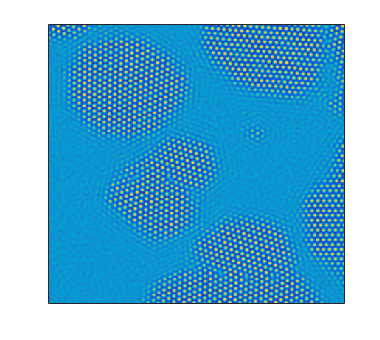
(a)

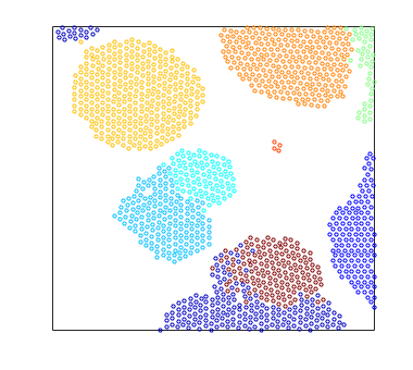
(b)

Figure 2: (a) shows a snapshot of the PFC density field $n$ in a small area of a simulation domain. (b) shows the corresponding detected peaks, grouped into clusters shown by color. Note that the method used to distinguish clusters does not always perfectly separate impinging clusters at their lattice boundaries. This is not an issue as we are interested in the number of such distinguishable clusters, rather than their exact final size.

A total of six data sets where obtained for this subsection. Each data set consists of the averaged results of 50 to 150 simulation runs. All data sets had fixed PFC model parameters $n_{o}=0.207$, $B^{x}=0.4$, and $N_{a}=0.040$. The effective PFC temperature $\Delta B$ increases between the data sets, chosen to be $\Delta B=0.16500+0.00025\epsilon$ for $\epsilon$ an integer from 0 to 5 corresponding to the six sets in order from first to last. The noise amplitude $N_{a}$ was chosen approximately within the recommended range corresponding to the other parameters as given in Ref. Kocher et al. (2016), bearing in mind that these authors’ results show that the variation range of $\Delta B$ between our data sets is too small to warrant a change in $N_{a}$ between the sets. Table 1 lists the data sets’ parameters and number of runs.

$\epsilon$	$\Delta B$	$B^{x}$	$n_{o}$	$N_{a}$	Number of runs
0	0.16500	0.4	0.207	0.040	100
1	0.16525	0.4	0.207	0.040	50
2	0.16550	0.4	0.207	0.040	50
3	0.16575	0.4	0.207	0.040	50
4	0.16600	0.4	0.207	0.040	150
5	0.16625	0.4	0.207	0.040	100

Table 1: PFC model parameters used to generate data sets $\epsilon=0$ to $\epsilon=5$. Also given is the number of simulation runs used to obtain the averaged results for each data set.

The parameters chosen for the aforementioned runs place the simulated systems below the solidus (at $\Delta B\approx 0.1685$ for the chosen $n_{o}$ and $B^{x}$) on the phase diagram, and above the instability curve (at $\Delta B\approx 0.1642$). The range of $\Delta B$ was chosen such as to allow appreciable amounts of nucleation to take place in a reasonable amount of computational time, while remaining above the instability curve. We note that this range is small relative to the range between the instability curve and the solidus, and that the range lies closer to the instability curve than to the solidus, indicating that the systems are greatly undercooled below their freezing point for nucleation to occur at noticeable rates. While this might be a result of making the PFC model’s equations dimensionless, there are some relevant physical systems exhibiting such homogeneous nucleation behaviour. For example, in the absence of heterogeneous nucleation, water is known to remain liquid at temperatures of $235K$ and below Langham and Mason (1958); Jeffery and Austin (1997). See also Hoyt (2001), where an estimate for the variation of $J_{ss}$ with temperature is obtained using realistic values for an alloy. This estimate predicts that the homogeneous nucleation rate is undetectable before a specific temperature more than $100K$ below the alloy’s freezing point, yet the rate rapidly increases beyond that specific undercooling temperature, similar to the behavior our results will show.

Figure 3 plots the post-critical nuclei densities $I^{*}(t)$, corresponding to the quantity in equation 20, for the first 5 sets. The sixth set, with $\epsilon=5$, is not visible on that figure’s scale. We observe that the early portion of these curves resembles the form predicted by CNT, such as in figure 1b, except that it is unclear whether the linearly increasing parts of these curves reach the true asymptote before tapering off to a constant value at late times due to the system fully transitioning to solid.

Figure 3: The post-critical nuclei densities for data sets $\epsilon=0$ to $\epsilon=4$. Time is in units of $dt$.

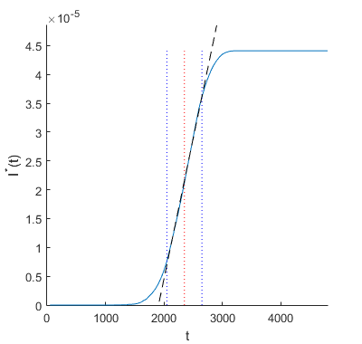
(a)

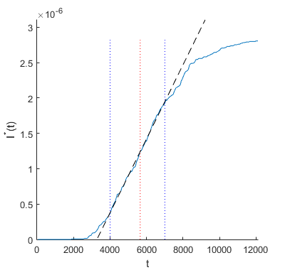
(b)

Figure 4: The geometric construction used to obtain $J_{ss}$ and $t^{*}$. Time is in units of $dt$. The vertical blue dotted lines indicate the time range encompassing the asymptote. The dashed black line is the linear fit over that time range. Also shown as a vertical red dotted line is the time at which 10% of the initial liquid volume has solidified. (a) Data set $\epsilon=0$, giving $J_{ss}=(4.9\pm 0.1)\times 10^{-8}$ and $t^{*}=1910\pm 70$. (b) Data set $\epsilon=4$, giving $J_{ss}=(5.23\pm 0.08)\times 10^{-10}$ and $t^{*}=3280\pm 90$. The errors on these values are from the uncertainty on the linear fit.

We obtain the steady-state rate of nucleation $J_{ss}$ and the incubation time $t^{*}$ by the geometric construction described in subsection III.2, taking as an assumption that the linear part of each data set’s $I^{*}(t)$ corresponds to the CNT-predicted asymptote. As a check for whether the assumption of asympoticity is sound, we also obtain for each data set the fraction of the initial liquid volume that transitioned to solid as a function of time. We find that in all the data sets, only 10% of the total liquid volume has solidified by the time approximately half of all post-critical nuclei have appeared. As the $I^{*}(t)$ curves have already entered the linear regime before that time, this suggests that the liquid has not yet been significantly depleted in the time range we assume to correspond to the asymptote. Figure 4 demonstrates the geometric constructions used to obtain $J_{ss}$ and $t^{*}$ for two of the data sets.

(a)

(b)

Figure 5: (a) Plot of $J_{ss}$ as a function of effective temperature $\Delta B$ for data sets $\epsilon=0$ to $\epsilon=5$ (blue circles), along with quadratic fit in semi-log space (red dashed line) showcasing faster than exponential decrease. Error bars are not visible at this scale. (b) Plot of $(\Delta G)^{-1}$ versus $\Delta B$, over the range $\Delta B$ for the data sets $\epsilon=0$ to $\epsilon=5$. Blue circles are calculated values, red dashed line is a linear fit.

Figure 5a plots $J_{ss}$ versus $\Delta B$ for the six data sets, on a semi-log plot. Also shown is a quadratic fit in semi-log space to demonstrate faster than exponential decrease of $J_{ss}$ as effective temperature $\Delta B$ increases. To compare this change in rate to equation 24, we only consider the effect of the exponential terms in that equation. As discussed in subsection III.3, we replace $k_{B}T$ by the dimensionless fluctuation temperature $T_{r}=N_{a}^{2}/2$, held constant since $N_{a}$ does not vary between the data sets. We also take $\Delta G_{A}$ and $\gamma$ (which are dimensionless due to the physical $k_{B}T$ having been scaled out) to be positive and decreasing as the effective temperature $\Delta B$ increases. We then turn to $\Delta G$ to try and explain the observed change in $J_{ss}$. Figure 5b plots $(\Delta G)^{-1}$ over the range of $\Delta B$ corresponding to the data sets, with $\Delta G$ estimated to be the difference between the solid and liquid bulk free energy densities of the PFC model, obtained from the standard one-mode approximation for the model. We observe that this plot varies approximately linearly with $\Delta B$, meaning $\Delta G$ can only account for at most exponential decrease, not faster than exponential. This suggests either that the CNT definitions of $\Delta G$, $\gamma$ or $\Delta G_{A}$ are inadequate for the PFC model, as mentioned in subsection III.3, or that the linear fit in the geometric construction used to obtain $J_{ss}$ was not at the true asymptote, which might have resulted in a lower bound for $J_{ss}$ that is less accurate for the data sets of lower $\epsilon$.

We believe the discrepancy mentioned in the previous paragraph is due to CNT’s assumption that the surface energy density $\gamma$ of a small forming grain is equivalent to the that of a much larger solid bulk’s interface. This assumption was what led us to take $\gamma$ as slowly decreasing with increasing model temperature, since that is the behavior of a solid bulk’s interfacial energy density both in the PFC model and in real crystalline materials. However, this assumption contradicts the existence of the instability curve of the model: in particular, equation 11 for the nucleation energy barrier $W^{*}$ implies that $\gamma$ must vanish for the nucleation barrier to vanish (since $\Delta G$ remains finite at the instability limit). Thus, the existence of the unstable region on the PFC model’s phase diagram (where by necessity the nucleation barrier must vanish) implies $\gamma$ for small grains must increase from zero at the instability curve to a higher value as effective temperature $\Delta B$ increases. The value of $\gamma$ for a nucleating grain then can not be the same as the interfacial energy density in a grain with a larger bulk, likely due to $\gamma$ including energetic contributions from effects such as high interface curvature which are not as significant for interfaces in larger grains. Taking as a new assumption that $\gamma$ of a small forming grain (near the instability curve) increases with temperature leads to qualitative agreement between equation 24 and the faster that exponential decrease of $J_{ss}$ seen in figure 5a.

We note that experiments for physical materials qualitatively support the predicted form of the $J_{ss}$ plot we obtained. For example, see figure 6 in Ref. Jeffery and Austin (1997) and figure 8a in Ref. LeGoues and Aaronson (1984), which respectively show steady state homogeneous nucleation rates for water and a CuCo alloy. These experiments observe a faster than exponential decrease as temperature increases on the high-temperature parts of these plots. A quantitative fit to experimental results using the PFC model is still an active area of research and is beyond the scope of this work. Further, we are unable to access the low-temperature regime of experimental plots using the PFC model described in this work, as the decrease in nucleation rate as temperature decreases requires a model with a temperature-dependent mobility.

Figures 6 plots $t^{*}$ for the aforementioned PFC data sets. We observe that $t^{*}$ increases with effective temperature $\Delta B$. Comparing to equation 25, the exponential term in that equation can not be the source of that increase under the assumptions that $k_{B}T$ is replaced by $T_{r}=N_{a}^{2}/2$ and $\Delta G_{A}$ decreases with the effective temperature parameter of the dimensionless PFC model. As figures 3 and 4 demonstrate, for our datasets, $J^{*}(0)\approx 0$ and thus we can safely assume that $K>0$ in equation 25. Using our new assumption that $\gamma$ increases with temperature as well as the variation of $(\Delta G)^{-1}$ from figure 5b, we can then conclude that the pre-exponential terms in equation 25 agree with the observed increase of $t^{*}$ with $\Delta B$, though no exact fit is attempted. This increase also agrees with the predictions for physical materials (for example, see the TTT curves of figure 1 in Ref. LeGoues and Aaronson (1984)), again for temperatures where temperature-dependent mobility is negligible.

Figure 6: Plot of incubation time $t^{*}$ for the PFC model data sets $\epsilon=0$ to $\epsilon=5$. Error bars were obtained from the uncertainty on the linear fit to the asymptote, as mentioned in figure 4.

IV.2 Nucleation rates and incubation times Vs. $N_{a}$

The data sets of subsection IV.1 allowed the comparison of nucleation in the PFC model to CNT as the effective temperature $\Delta B$ varied. The noise amplitude $N_{a}$ was taken to be coupled to the effective temperature $\Delta B$ as prescribed in Ref. Kocher et al. (2016), which led to $N_{a}$ being approximately constant over the small chosen range of $\Delta B$. It is of interest to examine the behavior of nucleation as a function of noise amplitude alone, to see whether our assumptions about the temperature dependence of exponential factors in equations 24 and 25 were warranted. In this section, we relax the requirement found in Ref. Kocher et al. (2016) on the noise amplitude parameter $N_{a}$, allowing it to be varied independently of $\Delta B$ over multiple new data sets. We stress that in these new data sets, $J_{ss}$ and $t^{*}$ curves are not expected to vary as would be predicted for a physical system, as decoupling the choice of $N_{a}$ from $\Delta B$ effectively leads to the thermal fluctuations being unphysical at the scale of the capillary length, as found in Ref. Kocher et al. (2016).

We generate six new data sets with fixed model parameters $n_{o}=0.207$, $B^{x}=0.4$, and $\Delta B=0.1650$, and with increasing noise amplitude $N_{a}=0.030+0.002\kappa$ for $\kappa$ an integer from 0 to 5 corresponding to the six sets respectively. Table 2 lists the parameters of the new data sets and number of runs for each.

$\kappa$	$\Delta B$	$B^{x}$	$n_{o}$	$N_{a}$	Number of runs
0	0.16500	0.4	0.207	0.030	100
1	0.16500	0.4	0.207	0.032	150
2	0.16500	0.4	0.207	0.034	50
3	0.16500	0.4	0.207	0.036	50
4	0.16500	0.4	0.207	0.038	50
5	0.16500	0.4	0.207	0.040	100

Table 2: PFC model parameters used to generate data sets $\kappa=0$ to $\kappa=5$. Also given is the number of simulation runs used to obtain the averaged results for each data set.

We repeat the procedure of subsection IV.1 for the new data sets. Figure 7 plots the post-critical nuclei densities $I^{*}(t)$ for each data set. Figures 8 and 9 plot $J_{ss}$ and $t^{*}$ for these data sets, respectively. Note that the x-axes for these two plots are in terms of $T_{r}=N_{a}^{2}/2$, the fluctuation temperature that enters the fluctuation-dissipation theorem as mentioned in subsection II.2.

Considering only the exponential terms of equation 24, and recalling that $\gamma$ and $\Delta G$ only vary with $\Delta B$, the observed variation of $J_{ss}$ is expected to be due to $\Delta G_{A}$ and the dimensionless fluctuation temperature of the PFC model, $T_{r}$. We attempt a fit of form $A_{1}\exp(-A_{2}/T_{r})$ to the plot of $J_{ss}$, where $A_{1}$ and $A_{2}$ are fit parameters, as shown in figure 8. The fit suggests agreement between equation 24 and our results, assuming that the factors of $1/T_{r}$ in the exponents are the main contributors to the variation of $J_{ss}$ over the considered range of $T_{r}$. The decrease of $\Delta G_{A}$ with increasing $T_{r}$ also possibly contributes to the observed increase in $J_{ss}$, though the effect of $1/T_{r}$ appears more prominently in the plot.

Figure 7: Post-critical nuclei densities for data sets $\kappa=0$ to $\kappa=5$. Time is in units of $dt$.

Figure 8: Plot of $J_{ss}$ for data sets $\kappa=0$ to $\kappa=5$ (blue circles), along with a fit of form $A_{1}\exp(-A_{2}/T_{r})$ for fit parameters $A_{1}=5.57\times 10^{-6}$ and $A_{2}=0.0036$ (red dashed line). Error bars are not visible at this scale.

Figure 9: Plot of $t^{*}$ for data sets $\kappa=0$ to $\kappa=5$. Error bars were obtained from the uncertainty on the linear fit to the asymptote.

As for incubation time, again due to $\gamma$ and $\Delta G$ not varying for these data sets, equation 25 indicates that $t^{*}$ would scale as $\exp(+\Delta G_{A}/k_{B}T)$ with $k_{B}T$ replaced by $T_{r}$ and $\Delta G_{A}$ decreasing with increasing $T_{r}$. Figure 9 shows a decrease in $t^{*}$ as $T_{r}$ increases, which suggests qualitative agreement with equation 25, though a specific fit was not attempted as the error bars allow both exponential as well as linear fits to be plausible.

IV.3 Appearance and growth of lattice structure in early grains

In CNT, the stochastically appearing grains are assumed to form with the same lattice structure as the final solid phase. Similarly, in the PFC model, the standard one-mode approximation for the solid phase also assumes the existence of well-defined lattice structure, as the PFC density $n(\vec{x})$ in the solid bulk can be expanded in terms of equal-amplitude Fourier wave modes corresponding to the lowest order reciprocal lattice vectors of the crystal structure (three wave modes for the case of a triangular lattice). However, it is feasible that free-standing planar waves or other non-lattice structures might temporarily appear in simulated PFC systems, especially during the early formation stages of solid grains (recall that amorphous structure has already been observed by other authors in both PFC model simulations Toth et al. (2010) as well as MD simulations Ozgen and Duruk (2004); Tian et al. (2008)). It is thus unclear whether the amplitude of all the one-mode approximation’s wave modes must fluctuate to a nonzero value simultaneously and symmetrically for a stable solid grain to form from a liquid phase, or whether the wave modes can separately appear and build up to a stable nucleus over time. To better understand this early stage of grain formation in terms of the wave modes, and also to assess whether non-lattice structures were prevalent in the simulation runs used to obtain the data sets the previous subsections, we use a field filtering method to examine the growth of separate wave modes during the early formation of a few grains in PFC simulations.

The field filtering method used in this subsection expands on work by Singer and Singer Singer and Singer (2006), where a method is developed to visualize the orientation of crystal grains in a fully solidified system. A ‘test wavelet’ is constructed, with a density field given by a one-mode approximation corresponding to one of the solid phase’s wave modes with a wave vector $\vec{q}$, multiplied to a Gaussian envelope. We convolve the test wavelet with the density field $n$ obtained from a simulation run, at a specific time $t$. This convolution enhances features of $n$ that exhibit the same structure as the wavelet. We then also apply a local averaging filter to smooth the wavelet-convolved $n$ field. The resulting filtered field’s value provides at each spatial location a relative estimate of the amplitude of the wave mode corresponding to the wavelet’s $\vec{q}$. By rotating the wavelet before applying this filtering process, the presence of a different wave mode can be examined at any location.

This filtering process is applied every few time steps of a nucleation-rate simulation, for a range of rotation angles, to obtain the relative amplitude of wave modes in the system as a function of time and position. We then store the values of the filtered fields at positions where nucleation occurs, taken to be the location of the first detected PFC density peak of each grain. Figure 10 plots the value of the filtered field at a specific location where a nucleation event was seen to occur, for a range of times and wavelet rotation angles, in a PFC system with model parameters corresponding to data set $\epsilon=4$ (see table 1 for the parameters). The three peaks that emerge correspond to the three wave modes expected in the final solid bulk with triangular lattice structure (note that these displayed mode peaks should not be confused with the PFC density peaks that represent the position of atoms in the system). At the final time shown ($t=9000$), the post-critical nucleus is known to have grown to a size much larger than the critical size, indicating that the values of the filtered field at that time are that of the final solid. We note that the height of the three peaks in the final solid are not equal as would be expected from the standard one-mode approximation for the PFC model. This is assumed to be due to numerical error, as the square numerical grid has 4-fold symmetry while the final lattice structure has 6-fold symmetry, leading to slight numerical anisotropy in the application of the convolution filter.

Figure 10: Value of the filtered field (y-axis) at the location of the first detected density peak of a forming grain, as a function of wavelet rotation angle (x-axis), for a range of times beginning before nucleation occurs and ending after the post-critical nucleus has grown to a size much larger than the critical size. The x-axis is in fractions of $\pi$. Time is in units of $dt$.

Once the angles for the peaks of the filtered field of a nucleation event are known at late times, we can plot the growth versus time of the field for only these three angles starting from early times. Figure 11 plots the growth of these peaks for two nucleation events, with parameters corresponding to data set $\epsilon=0$ in table 1. The values are normalized with respect to the maximum value attained by each peak, to account for the mentioned inequality of the peaks at late time due to numerical anisotropy. We also examined other nucleation events and obtained similar plots to these two cases.

(a)

(b)

Figure 11: Normalized values of the filtered field (y-axis) at the angles corresponding to the the peaks in the filtered field associated with a nucleation event (corresponding to the three colours shown: red, yellow, and blue), as a function of time (in units of $dt$), for two separate nucleation events in the same simulated system.

Figure 12: Density field of the grain from which filtered field peak values shown in figure 11b where obtained, at simulation time $t=2550$. Axes indicate grid points.

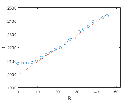
Figure 13: Simulation time taken for the density field of a forming grain to achieve half the maximum time correlation of the late-time (post full solidification) density field of that grain. The x-axis is radius in units of $dx$. The y-axis is time in units of $dt$. Blue circles are radial averages of the time taken, and red line is a linear fit to the large-radius averages.

The filtered field values at the three peak positions appear to vary in tandem during the majority of the process (up to the order of thermal fluctuations). This leads us to conclude that, at least for the parameter ranges of the data sets of section IV.1, nucleation in the PFC model exhibits a triangular atomic lattice structure even during the relatively early parts of grain formation. However, a minority of examined grains display unexpected behavior of the filtered field values at the three peaks, such as the grain corresponding to figure 11b. In that figure, the black arrow points to a relatively large fluctuation of only one mode that appears to precede the rapid growth of all three modes. The dashed lines denote a range of time where the three modes’ growth seems to be delayed at a value higher than the liquid background value, yet lower than the final solid value. We believe these behaviors are due to a few grains forming with more complex forms, unaccounted for in our assumptions. Figure 12 shows the grain corresponding to figure 11b. We observe that this grain appears to exhibit two separate lattice orientations. This is possibly due to it being formed from two grains that merged into one at an earlier time. Another possible explanation is the existence of a precursor non-crystalline phase or preferred structure that precedes the critical nucleus. The competition between these separate lattice orientations might explain the growth delay observed in figure 11b, as well as the single mode fluctuation before the final rapid growth.

These results indicate that the developed wave mode analysis method requires further refinement to be able to distinguish such edge cases. They also offer more insight into the difficulties involved in applying CNT to nucleation in the PFC model, as these complex-structured grains violate CNT’s no-interaction or crystalline-structure assumptions, likely extending the required time for these grains to achieve criticality as their lattice structures stabilize.

While the method above characterized the appearance of structure in grains by examining the growth of modes at only the first PFC density peak appearing in grains, we also briefly studied the spatial dependence of structure formation. By calculating the time correlation of the late-time (post full solidification) density field $n$ with earlier time values of the field, we obtain the relative rate of formation of lattice structure at spatial grid points at and near the forming grain. Figure 13 plots the average simulation time taken for the PFC density in a grain to achieve half its maximum time correlation with its late-time value, as a function of radial distance from the approximate center of the grain. The chosen grain was nearly circular, to ensure validity of radial averaging. We observe that, below a radius of approximately $10\,dx$ (corresponding to $1.25a$), the grain’s structure approaches that of the final solid at a time independent of radius. Above this radius, information of the final lattice structure spreads linearly with time, as would be expected of a post-critical grain growing with constant interface velocity. The radius where this crossover behaviour occurs can be argued to be equivalent to the critical nucleus radius for the PFC model for the particular set of parameters used. This result provides further evidence that the appearance of a post-critical grain in the PFC model is preceded by fluctuation-induced lattice structure instantaneously appearing over a finite simulation volume. Though this method could in principle be repeated for a large number of circular grains at multiple simulation parameters to obtain statistics and parameter dependence for the critical radius, we do not attempt to do so in this work due to the difficulty in obtaining large numbers of sufficiently circular grains.

IV.4 Numerical approximation for the form of critical nuclei

As discussed in subsection III.3, we expect that the form of critical nuclei in the PFC model does not depend on only the number of atoms in an emerging grain, as assumed by CNT. We thus develop a method to efficiently numerically approximate the form of critical nuclei in the PFC model under the slightly more flexible assumption that both size and order of a grain can vary during the nucleation process. Note that Toth et al. Toth et al. (2010) have previously examined the work of formation of critical nuclei by solving the Euler-Lagrange equation of the PFC model to obtain local extrema of the free energy functional. However, in this work we instead obtain approximate forms of the critical nuclei by numerically testing whether a constructed ‘test grain’ of a given form is stable in a system with no fluctuations. While our method does not allow the reconstruction of the nucleation energy barrier, it provides insight on possible kinetics paths for a grain to attain criticality.

We start by constructing a ‘test grain’, whose density field follows the lattice structure of a bulk PFC solid in the one-mode approximation, multiplied to a Gaussian envelope centered on one of the peaks. The amplitude of the test grain’s density field is set to $r_{1}\phi_{s}$, where $\phi_{s}$ is the amplitude predicted in a stable solid bulk at the system’s position on its phase diagram, and $r_{1}$ is a value between 0 and 1. Similarly, the standard deviation of the Gaussian envelope is set to $r_{2}a$ where $a$ is the dimensionless lattice constant and $r_{2}>0$. Figure 14 shows a grain that formed stochastically in a simulated PFC run, as well as a comparable test grain constructed as explained above.

Effectively, the parameter $r_{1}$ sets the relative order of the grain with respect to the original liquid and final solid phases, while $r_{2}$ determines the size of the grain. The parameter $r_{1}$ can also be heuristically understood as determining the average number of vacancies in the lattice of the forming grain, as it has been argued Berry et al. (2014) that variations in the amplitude of the PFC model’s periodic density field can represent vacancy diffusion on diffusive time scales. We note that this approximate grain construction is only expected to be valid for small-radius grains; large stable solid grains would have a constant amplitude throughout their bulk and a finite interface width, rather than an approximately Gaussian profile for the amplitude. Furthermore, this construction does not account for a variation in average density of the grain’s interior, as the constructed periodic field would average to $n_{o}$ over a large enough bulk.

(a)

(b)

Figure 14: (a) Solid grain surrounded by fluctuating liquid, observed in a simulation run with PFC model parameters $n_{o}=0.207$, $B^{x}=0.4$, $\Delta B=0.1650$, and $N_{a}=0.04$. (b) Constructed grain with same model parameters as (a) (without fluctuations), and with chosen parameters $r_{1}=0.5$ and $r_{2}=0.8$. In both figures, the x-axis and y-axis are in number of grid points, and the color bar shows the value of the density fields.

For a given set of PFC model parameters and chosen $r_{1}$ and $r_{2}$, we can test whether a constructed test grain is post-critical or pre-critical by simulating it in a system consisting of the single grain in a much larger amount of liquid phase. The fluctuation amplitude is set to zero in this simulation, as the grain is assumed to be the result of a prior fluctuation, and we are interested in the subsequent deterministic evolution of this grain. If after sufficient time steps the grain has grown to fill the system with solid, then it is known to be a post-critical grain, and vice versa. By repeating this test for various $r_{1}$ and $r_{2}$ (using a half-interval search method in one of the two variables, for efficiency), we obtain a curve in the space spanned by these two parameters that determines whether a grain with specific $r_{1}$ and $r_{2}$ is post-critical. We refer here to this curve as ‘critical nucleus curve’. The exact form of the critical nucleus is thus not unique, as any set of $r_{1}$ and $r_{2}$ lying on such a curve would give a critical nucleus under the assumptions of the construction used.

We numerically calculate the critical nucleus curves for the parameters of data sets $\epsilon=0$ to $\epsilon=5$ (see table 1 for the parameters). Figure 15 shows these curves. Note that data sets $\kappa=0$ to $\kappa=5$ (see table 2 for the parameters) would have the same critical nucleus curve as data set $\epsilon=0$, as these curves do not depend on fluctuation amplitude $N_{a}$. We observe that, as $\epsilon$ (equivalently, the effective temperature $\Delta B$) increases, the curves shift along both the relative order axis (y-axis) and size axis (x-axis). The shift along the size axis agrees with the basic prediction of CNT that critical radius must increase with temperature. However, CNT does not account for the shift along the order axis, as it assumes the lattice structure in the interior of the grain is always the same as that of the final solid. Further, the precise kinetic path that a forming grain would take through $(r_{1},r_{2})$ parameter space before becoming a post-critical nucleus can not be predicted by CNT. This would instead require at least a 2 parameter theory similar to that developed in Ref. Lutsko and Duran-Olivencia (2015) for the case of nucleation in globular protein systems. We expect that the most likely path to criticality will depend on a balance between statistically probable fluctuation amplitude and diminishing spatial correlation at long range. Specifically, a critical nucleus of too small radius is unlikely to form due to the exponentially decreasing odds of obtaining a sufficiently large fluctuation as the required field amplitude increases, while a critical nucleus of too large radius is unlikely to form before smaller grains because the spatially conserved density fluctuations in the system limit the rate at which mass and information of the forming lattice structure can propagate at large distances. This appears to be supported by the data in Figure 13, which suggests a magnitude for this correlation length, and hence $r_{2}$.

Figure 15: Critical nucleus curves for data sets $\epsilon=0$ to $\epsilon=5$. Grains with values of $(r_{1},r_{2})$ above the corresponding system’s curve are post-critical. Recall that $r_{1}$ is a ratio that scales the amplitude of the periodic density field of the grain, while $r_{2}$ scales the radius of the Gaussian-shaped grain.

V Conclusion

The goals of this work were to examine time-dependent nucleation statistics in the PFC model and attempt a comparison with the predictions of CNT. We have shown that the PFC model follows the qualitative predictions of CNT. For fluctuations parameterized with model temperature such as to ensure correct capillary fluctuations Kocher et al. (2016), homogeneous nucleation was found to occur at strong undercoolings. The rate of nucleation was observed to not be constant, instead requiring a transient time to achieve its steady state behavior. The steady state rate of nucleation was shown to decrease at least exponentially as temperature increased, while incubation time was shown to increase nearly linearly with temperature (although no actual fit was attempted). All these behaviors were also argued to be qualitatively consistent with experimental nucleation rate predictions and results, within the constraint of negligible temperature dependence of mobility. Quantitative agreement with experiments would require significant tuning of the model that is beyond the scope of this work. Our results indicate that the PFC model can be used to study solidification phenomena that might require prior nucleation to initialize grain number density, such as structure growth, grain coalescence, and Ostwald ripening.

Our results also showcased the CNT-predicted dependence of the steady state nucleation rate and incubation time explicitly on fluctuation amplitude. Despite the PFC model not including a direct equivalent of the CNT-assumed activation energy for atoms jumping through phase interfaces, the steady state nucleation rate was shown to vary with fluctuation amplitude following a dependence agreeing with that predicted for a thermally activated process. Similarly, the incubation time was seen to decrease as fluctuation amplitude increased, as expected in a system where propagation of mass and information is limited by the amplitude of spatially conserved density fluctuations.

Finally, we also studied some of the limitations of CNT as applied to the PFC model. We examined the wave mode amplitudes in pre-critical grains, observing that, despite lattice structure appearing early on in the process for most grains, a minority of nucleation events displayed more complicated structural formation behavior that might affect the validity of growth rate and non-interaction assumptions used in CNT. We also numerically calculated ‘critical nucleus curves’ to examine the approximate form of critical nuclei in the PFC model, under the assumption that both size and order of a grain are allowed to vary. These curves indicated that the CNT assumption of a single-parameter dependence (nucleus size) is likely insufficient to consistently predict nucleation in PFC. We suggest that a multi-parameter theory should be attempted, similar to the work in Ref. Lutsko and Duran-Olivencia (2015). In the case of the PFC model, the parameters required might include some or all of the following: grain size, relative order compared to final solid state, local average density, and interface width.

References

- Jin et al. (2003) L. Jin, K. A. Claborn, M. Kurimoto, M. A. Geday, I. Maezawa, F. Sohraby, M. Estrada, W. Kaminksy, and B. Kahr, Proceedings of the National Academy of Sciences 100, 15294 (2003).
- Granasy et al. (2006) L. Granasy, T. Pusztai, and T. Borzsonyi, Handbook of Theoretical and Computational Nanotechnology, Vol. 9 (American Scientific Publishers, 2006) pp. 525–572.
- Boettinger et al. (2000) W. Boettinger, S. Coriell, A. Greer, A. Karma, W. Kurz, M. Rappaz, and R. Trivedi, Acta Materialia 48, 43 (2000).
- David et al. (2003) S. A. David, S. S. Babu, and J. M. Vitek, JOM 55, 14 (2003).
- Kurz et al. (2001) W. Kurz, C. Bezencon, and M. Gaumann, Science and technology of advanced materials 2, 185 (2001).
- Granasy et al. (2002) L. Granasy, T. Borzsonyi, and T. Pusztai, Phys. Rev. Lett. 88, 206105 (2002).
- Hohenberg and Halperin (1977) P. C. Hohenberg and B. I. Halperin, Rev. Mod. Phys. 49, 435 (1977).
- Singer-Loginova and Singer (2008) I. Singer-Loginova and H. M. Singer, Reports on Progress in Physics 71, 106501 (2008).
- Chaikin and Lubensky (1995) P. M. Chaikin and T. C. Lubensky, Principles of condensed matter physics (Cambridge University Press, 1995).
- (10) N. Provatas and K. Elder, Phase-Field Methods in Material Science and Engineering (Wiley-VCH).
- Elder et al. (1994) K. R. Elder, F. Drolet, J. M. Kosterlitz, and M. Grant, Phys. Rev. Lett. 72, 677 (1994).
- Folch and Plapp (2005) R. Folch and M. Plapp, Phys. Rev. E. 72, 011602 (2005).
- Hotzer et al. (2015) J. Hotzer, M. Jainta, P. Steinmetz, B. Nestler, A. Dennstedt, A. Genau, M. Bauer, H. Kostlerc, and U. Rudec, Acta Materialia 93, 194 (2015).
- Karma and Rappel (1997) A. Karma and W.-J. Rappel, Preprint (1997).
- Provatas et al. (1998) N. Provatas, N. Goldenfeld, and J. Dantzig, Phys. Rev. Lett. 80, 3308 (1998).
- Kim et al. (1999) Y. Kim, N. Provatas, N. Goldenfeld, and J. Dantzig, Phys. Rev. E 59, R2546 (1999).
- Karma (2001) A. Karma, Phys. Rev. Lett. 87, 115701 (2001).
- Echebarria et al. (2004) B. Echebarria, R. Folch, A. Karma, and M. Plapp, Phys. Rev. E. 70, 061604 (2004).
- Greenwood et al. (2004) M. Greenwood, M. Haataja, and N. Provatas, Phys. Rev. Lett. 93, 246101 (2004).
- Ramirez et al. (2004) J. C. Ramirez, C. Beckermann, A. Karma, and H. J. Diepers, Phys. Rev. E 69, 051607 (2004).
- Echebarria et al. (2010) B. Echebarria, A. Karma, and S. Gurevich, Phys. Rev. E 81, 021608 (2010).
- Amoorezai et al. (2010) M. Amoorezai, S. Gurevich, and N. Provatas, Acta Materialia 58, 6115 (2010).
- Karma et al. (2001) A. Karma, D. A. Kessler, and H. Levine, Physical Review Letters 87, 045501 (2001).
- Li et al. (2017) Y. Li, S. Hu, X. Sun, and M. Stan, npj Computational Materials 3, 16 (2017).
- Elder et al. (2001) K. R. Elder, M. Grant, N. Provatas, and J. M. Kosterlitz, Phys. Rev. E 64, 021604 (2001).
- Plapp (2011) M. Plapp, Philosophical Magazine 91, 25 (2011).
- Ofori-Opoku and Provatas (2010) N. Ofori-Opoku and N. Provatas, Acta Materialia 58, 2155 (2010).
- Steinbach and Apel (2006) I. Steinbach and M. Apel, Physica D: Nonlinear Phenomena 217, 153 (2006).
- Montiel et al. (2012) D. Montiel, L. Liu, L. Xiao, Y. Zhou, and N. Provatas, Acta Materialia 60, 5925 (2012).
- Alder and Wainwright (1959) B. J. Alder and T. E. Wainwright, The Journal of Chemical Physics 31, 459 (1959).
- Rapaport (2004) D. C. Rapaport, The Art of Molecular Dynamics Simulation (Cambridge University Press, 2004).
- Ozgen and Duruk (2004) S. Ozgen and E. Duruk, Materials Letters 58, 1071 (2004).
- Tian et al. (2008) Z. Tian, R. Liu, H. Liu, C. Zheng, Z. Hou, and P. Peng, Journal of Non-Crystalline Solids 354, 3705 (2008).
- Hoyt et al. (2001) J. J. Hoyt, M. Asta, and A. Karma, Phys. Rev. Lett. 86, 5530 (2001).
- Shibuta et al. (2015) Y. Shibuta, K. Oguchi, T. Takaki, and M. Ohno, Scientific Reports 5, 13534 (2015), article.
- Elder et al. (2002) K. R. Elder, M. Katakowski, M. Haataja, and M. Grant, Phys. Rev. Lett. 88, 245701 (2002).
- Elder and Grant (2004) K. R. Elder and M. Grant, Phys. Rev. E 70, 051605 (2004).
- Elder et al. (2007) K. R. Elder, N. Provatas, J. Berry, P. Stefanovic, and M. Grant, Phys. Rev. B 75, 064107 (2007).
- Emmerich et al. (2012) H. Emmerich, H. Lowen, R. Wittkowski, T. Gruhn, G. I. Toth, G. Tegze, and L. Granasy, Advances in Physics 61, 665 (2012).
- Humadi et al. (2013) H. Humadi, N. Ofori-Opoku, N. Provatas, and J. J. Hoyt, JOM 65, 1103 (2013).
- Berry et al. (2008) J. Berry, K. R. Elder, and M. Grant, Phys. Rev. B 77, 224114 (2008).
- Berry et al. (2012) J. Berry, N. Provatas, J. Rottler, and C. W. Sinclair, Phys. Rev. B 86, 224112 (2012).
- Berry et al. (2014) J. Berry, N. Provatas, J. Rottler, and C. W. Sinclair, Phys. Rev. B 89, 214117 (2014).
- Tupper and Grant (2008) P. F. Tupper and M. Grant, EPL (Europhysics Letters) 81, 40007 (2008).
- Radhakrishnan et al. (2012) B. Radhakrishnan, S. B. Gorti, D. M. Nicholson, and J. Dantzig, Journal of Physics: Conference Series 402, 012043 (2012).
- Toth et al. (2010) G. I. Toth, G. Tegze, T. Pusztai, G. Toth, and L. Granasy, Journal of Physics: Condensed Matter 22, 364101 (2010).
- Granasy et al. (2011) L. Granasy, G. Tegze, G. I. Toth, and T. Pusztai, Philosophical Magazine 91, 123 (2011).
- Ramakrishnan and Yussouff (1979) T. V. Ramakrishnan and M. Yussouff, Phys. Rev. B 19, 2775 (1979).
- Greenwood et al. (2010) M. Greenwood, N. Provatas, and J. Rottler, Phys. Rev. Lett. 105, 045702 (2010).
- Wu et al. (2010) K.-A. Wu, M. Plapp, and P. W. Voorhees, Journal of Physics: Condensed Matter 22, 364102 (2010).
- Greenwood et al. (2011) M. Greenwood, N. Ofori-Opoku, J. Rottler, and N. Provatas, Phys. Rev. B 84, 064104 (2011).
- Mandel et al. (1970) F. Mandel, R. J. Bearman, and M. Y. Bearman, The Journal of Chemical Physics 52, 3315 (1970).
- Garcia-Ojalvo and Sancho (1999) J. Garcia-Ojalvo and J. M. Sancho, Noise in Spatially Extended Systems (Springer, 1999).
- Kocher et al. (2016) G. Kocher, N. Ofori-Opoku, and N. Provatas, Phys. Rev. Lett. 117, 220601 (2016).
- Hoyt (2001) J. J. Hoyt, Phase Transformations (Cambridge University Press, 2001).
- Sear (2007) R. P. Sear, Journal of Physics: Condensed Matter 19, 033101 (2007).
- Shi et al. (1990) G. Shi, J. H. Seinfeld, and K. Okuyama, Phys. Rev. A 41, 2101 (1990).
- LeGoues and Aaronson (1984) F. K. LeGoues and H. I. Aaronson, Acta Metallurgica 32, 1855 (1984).
- Lutsko and Duran-Olivencia (2015) J. F. Lutsko and M. A. Duran-Olivencia, Journal of Physics: Condensed Matter 27, 235101 (2015).
- Jeffery and Austin (1997) C. A. Jeffery and P. H. Austin, Journal of Geophysical Research 102, 25 (1997).
- Langham and Mason (1958) E. J. Langham and B. J. Mason, Proceedings of the Royal Society of London. Series A, Mathematical and Physical Sciences 247, 493 (1958).
- Singer and Singer (2006) H. M. Singer and I. Singer, Phys. Rev. E 74, 031103 (2006).